複雜網路中的小世界和群聚性基調

國立交通大學

資訊科學系

碩士論文

複雜網路中的小世界和群聚性基調

Small-world and Clustering Motifs in

Complex Networks

研 究 生：鄭家胤

指導教授：孫春在 教授

在複雜網路中小世界和群聚性基調

學生:鄭家胤

指導教授：孫春在

國立交通大學

資訊科學研究所

摘要

Small-world and Clustering Motifs in

Complex Networks

Student:

Advisor:

Institute of Computer and Information Science

National Chiao-Tung University

Abstract

Recently many researches found obvious local clustering property and small-world property in various kinds of complex world. To understand the detailed structure and specific dynamic properties of various networks and to classify the key differences of various similar networks, we defined two kinds of different network motifs in topology and function according to the link property of edge. These two network motifs are small-world motifs and clustering motifs which are functionally important and statistically significant. By discovering and analyzing these two kinds of motifs, researchers in many fields of science can not only understand completely the global information and local structure of real networks but also the construction and evolution beyond the network.

Content

摘要... ii

Abstract ... iii

3.1 Definition of weight of edge ...10

3.2 Definition of weak-ties and strong -ties... 11

3.3 Definition of small-world motif and clustering motif... 11

3.4 Small-world and clustering motif Detection...12

3.5 Comparison among different networks...12

4 Experiment and Result...14

4.1 A network with small-world motifs and clustering motifs ...14

4.2 A network with only small-world motifs ...16

4.3 A network with only clustering motifs...16

4.4 Compare different networks ...17

4.5 Explore the details of each complex network ...18

5 Conclusion ...19

Reference ...21

6 附錄 A...23

Generation of Random Network...23

Controlling for Appearances of (n-1)-Node Motifs ...23

Network Motif Detection...24

Compare among different Networks...24

附錄 B...25

Table

TABLE 1.13 TYPES OF MOTIFS OF SIZE 3[6] ...8

TABLE 2.NETWORK MOTIFS FOUND IN BIOLOGIVAL AND TECHNOLOGICAL NETWORKS. ...15

TABLE 3.THE DETAILS OF THE NETWORKS...25

TABLE 4.THE DETAILS OF THE MOTIFS IN EACH NETWORK...27

TABLE 5.YEAST的 ZSCORE和 SUPERFAMILY...28

TABLE 6.LEADER的 ZSCORE和 SUPERFAMILY...29

TABLE 7.PRISONER的 ZSCORE和 SUPERFAMILY...30

TABLE 8.YTHAN的 ZSCORE和 SUPERFAMILY...31

TABLE 9.ST.MARTIN的 ZSCORE和 SUPERFAMILY...32

TABLE 10.CHESSPEAKE的 ZSCORE和 SUPERFAMILY...33

TABLE 11. COACHELLAINTER的 ZSCORE和 SUPERFAMILY...34

TABLE 12.LITTLEROCK的 ZSCORE和 SUPERFAMILY...35

TABLE 13.B.BROOK的 ZSCORE和 SUPERFAMILY...36

TABLE 14.SKIPWITH的 ZSCORE和 SUPERFAMILY...37

TABLE 15.S208 的 ZSCORE和 SUPERFAMILY...38

TABLE 16.S420 的 ZSCORE和 SUPERFAMILY...39

Figure

FIGURE 1.ONE SPECIAL CASE IN SOCIAL COMMUNITY. ...5

FIGURE 2.NETWORK MOTIFS FOUND IN THE E.COLI TRANSCRIPTIONAL REGULATION NETWORK [11] ...7

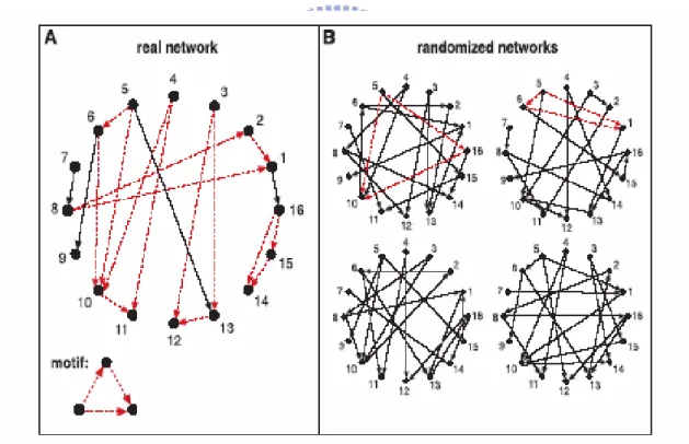
FIGURE 3.A)A REAL NETWORK,B) SIMILAR RANDOM NETWORKS...8

FIGURE 4.THE CURVE OF THE NORMALIZED Z SCORE THOROUGH MILO’S MOTIF AND CLASSIFICATION..17

FIGURE 5.THE CURVE OF THE NORMALIZED Z_SMALLWORLD SCORE THROUGH SMALL-WORLD MOTIF AND CLASSIFICATION...18

FIGURE 6.THE CURVE OF THE NORMALIZED Z_CLUSTERING SCORE THROUGH CLUSTERING MOTIF AND CLASSIFICATION...18

FIGURE 7.YEAST的 SUPERFAMILY...28

FIGURE 8.LEADER的 SUPERFAMILY...29

FIGURE 9.PRISONER的 SUPERFAMILY...30

FIGURE 10.YTHAN的 SUPERFAMILY...31

FIGURE 12.CHESSPEAKE的 SUPERFAMILY...33

FIGURE 15.B.BROOK的 SUPERFAMILY...36

FIGURE 17.GENERAL FEEDBACK STRUCTURE...38

1 Introduction

In the twentieth century, complexity is a new science which includes not only the meaning of the word, but also in fact “complex and various” and “organization and structure”. We can divide the physical world into three different systems. The first is the “regular” system which is stable and periodic, like Newton’s celestial mechanics. The second is the “Chaos” system which is composed of many chaotic molecules, like gas molecules. The third is between regular and Chaos, like structured and infinite varied features in ecosystem, economy, politics, or psychology. Complexity will face the challenge of the third. To research this kind of question, many complex structures are represented by the network which is so-called “complex network”. This complex network goes from scale of biomolecules, through cells, to organisms, such as: transcription network, neuron synaptic connection network and ecological food web.

The research of complex network is a high multi-sciences, and the sources of the network’s data are all-inclusive and much wider than any other science’s range, from Science Corporation, movie production, food web chains evolution, contagious disease spread, to document connection. The characteristic of this kind of research is data validation, math theory deduction, and the high integrity of computer simulation. Most of network data and structure are too large and complex to transform them to strict mathematical description. Therefore computer simulation became an accredited scientific verification, but how to collect useful information is a worth-discussed topic. Many scientists interest in how to discover the law or structure beyond the network. For example, the rivers which are different in appearance may be created by the rainfall of the climate and minerals which form mountains and plains. But on the view of rivers’ catchments and the

number of rivers, we found that they follow “power-law”, which shows that the number of rivers decrease 2.7 times[1] while the square measure of rivers’ catchments area is doubled. Another example is that of mail experiments by Milgram who discovered “six-degree of separation [2]”. This shows that any two among six hundred million people can connect to each other through on average six people. This discovering of the objective law in the network also provides us another shortcut of solving or analyzing problems. For instance, in www network, when analyzing in link property, data mining (like: page rank), sociology of content creation and detection of communication can be found out [20]. Therefore, with a good network model and full understanding of the network structure, we can 1) prove formal properties of algorithm, 2) detect the peculiar region of the network, and 3) predict evolution of new phenomena.

Analyzing network typology can help researchers solve many problems in complex network [3]. For example, the reasons that cause Milgram’s “six degree of separation” is “small-world [4]”, scale-free network shows the order of the unorderly www network and “preferential attachment” is the reason why most wealth is in the hand of few people. This global information of the network helps us compare the properties of many different networks.

However when we look further into the detailed structure of network or the structural design principles of network, this kind of global information is not sufficient. We noticed that Milo’s research defined “motifs” as patterns of interconnections occurring in complex networks at numbers that are significantly higher than those in randomized networks. After finding motifs according to local structure, Milo added some function to them. However, opinions are divergent on this point [7].

functionalities of these networks, we referred to Mark’s weal tie proposal[8] and defined the “small-world” and “clustering” motifs which are network simple building blocks with weak or strong ties. We found such small-world motif in networks from neurobiology to ecology to engineering. In those networks, small-world motif plays an important role which substantially lowers the degree of separation of the network by its “weak tie”. We modify Milo’s motifs [7] by adding the “weak” or “strong” properties on the edges of those motifs to analyze more functionalities and differences between them. For instance, both gene regulation network and social network have similar Feed-Forward loop motif in Milo’s previous research. However, we found the small-world Feed-Forward loop motif in gene regulation network but clustering Feed-Forward loop motif in social network. The clustering Feed-Forward loop is far from the former owing to the clustering in the latter. Moreover, by finding the motifs statistically and functionally significant, we show both local structure and global information in individual complex network.

The rest of this paper is organized as follows: in the next section we will discuss research on small-world, weak tie and motif. The third section details how we adopt the Milo’s and Mark’s researches to build our model. We first defined the strong-tie and weak-tie of the edge, two kinds of motifs, methods of how to find out motifs, and finally comparisons between different networks. In the forth section, we experimented with five kinds of complex networks. In the fifth section, we discuss how to complex networks into three types according to small-world motif or clustering motif that existed in complex networks. Finally, we

summarized our contribution and discussed some unsolved problems in future work.

2 Related works

2.1 Small worlds

Since the middle age of 1960, “small world phenomenon” has been found again and again, for instance, Milgram discovered “six degree of separation” through mail experiments [2] and “Oracle of Kevin Bacon”---if any two persons show together in the same movie, and we say these two are connected. For instance, how many connections are between Elvis Presley and Kevin Bacon? In the movie”Speedway (1968)” Elvis Presley and”Courtney Brown” showed together, and the latter showed in”My Dog Skip (2000)” with Bacon. So there is only one step space between Elvis Presley and Bacon. The average separation between each actor and Bacon is 2.896. This small world phenomenon exists almost everywhere. However, there isn’t a real model can be used to explain this specific phenomenon until 1996. Watts and Strogatz provided “small-world model [4]”, which begins with a regular network and then we can add some links (shortcuts) randomly. They found that the fewer short cuts you add the less effects the clustering got.

2.2 Weak-ties

When small world phenomenon is represented, it attracted many people, sociologist Granovetter is one of them, and he strongly felt that a worth-discussed is hided behind the small world phenomenon. In 1973, Granovetter’s paper “the strength of the weak ties [8]” revealed this secrete to the world. Granovetter firstly researched “what kind of link connects the community”. He roughly mentioned the strength of connection among people. For example, we and our family or our friends are often together, this

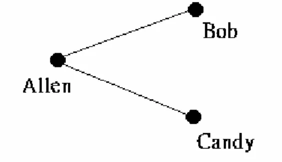
connection is “strong tie”, while “weak-tie” is for the connection between us and nodding acquaintances. Granovetter wanted to discuss whether the key connection is strong-tie or weak-tie. Take following graph as consideration:

Figure 1. One special case in social community.

If Allen has a strong tie with Bob and Candy, then the possibility that Bob has a strong tie with Candy is very high. In this special case, strong-tie connections usually seldom exist alone, but instead, they formed triangles easily. For example, both of my good friends, in real life, are usually good friends. Therefore, in relationship network, removing a strong-tie connection is hard to affect the degree of separation of the network. It is because that we can get to the other point through the left two edges in this strong-tie-formed triangle. Therefore, oppose to our general concept, strong-tie connection is not the key for maintaining the network. But instead, weak-tie connection plays a different role which like a “bridge”. If this bridge disappears, it will be very hard to connect between the points in the one side of the bridge with that point in the other side. Weak-tie connection plays a key role in maintaining networks. For example, in real life, Granovetter discovered that 16% people found jobs through people they “often” met, while 84% people found jobs through people they ”seldom” met. It’s easy to send the message to other people that we want jobs, but it isn’t far enough. Your good friend might have heard this news for two or three times from your common friends.

But a distant relative or a nodding acquaintance might pass it on to further. Granovetter’s conclusion is that weak-tie connection is an important factor maintaining the small world which has a low degree of separation. Without weak-tie connection, the whole network will be divided into separated disconnected groups. Weak-tie connection is not only a key connection between individuals, but also in groups.

2.3 Clustering

Clustering is a common phenomenon in nature, for example, in human relationship; we often interacted with our neighbors or people near us and finally formed a group. In the prior research, “clustering algorithm” is always an important issue.

Clustering can be considered the most important unsupervised learning problem; so, as every other problem of this kind, it deals with finding a

structure in a collection of unlabeled data. A loose definition of clustering

could be “the process of organizing objects into groups whose members are similar in some way”. A cluster is therefore a collection of objects which are “similar” between them and are “dissimilar” to the objects belonging to other clusters. So, the goal of clustering is to determine the intrinsic grouping in a set of unlabeled data. But how to decide what constitutes a good clustering? It can be shown that there is no absolute “best” criterion which would be independent of the final aim of the clustering. Consequently, it is the user which must supply this criterion, in such a way that the result of the clustering will suit their needs.

For instance, we could be interested in finding representatives for homogeneous groups (data reduction), in finding “natural clusters” and describe their unknown properties (“natural” data types), in finding useful

and suitable groupings (“useful” data classes) or in finding unusual data objects (outlier detection).

2.4 Motif

The earliest application of network motifs is in gene regulation network [11], and finding basic building blocks which has the property of the clustering in complex wiring diagram. These building blocks can divide into three types: feedforward loop, single input module (SIM), dense overlapping regulons (DOR)) (Figure 2).

Figure 2. Network motifs found in the E.coli transcriptional regulation network [11]

Milo expanded this method [6] and defined 13 types of motif which size=3(Table 1). This motif still has clustering property.

ID 6 12 14 36 38 46 74 78 98 102 108 110 238

Motif

Table 1. 13 types of motifs of size 3[6]

In real network, the frequency of occurrences of each subgraph was recorded. Milo compared the real network to suitably randomized networks and only selected patterns appearing in the real network at numbers significantly higher than those in the randomized networks to be motif.

Figure 3. A) A real network, B) similar random networks

For a stringent comparison, Milo used randomized networks (Figure 3) that have the same single-node characteristics as does the real network: Each node in the randomized networks has the same number of incoming and

outgoing edges as the corresponding node in the real network. Furthermore, the randomized networks used to calculate the significance of n-node subgraphs were generated to preserve the same number of appearances of all (n-1)-node subgraphs as in the real network (See Appendix A).

To compare the different networks, Milo described the statistical significance as Z score and defined Superfamily(SP) which is the vector of Z scores normalized to length 1 (See Appendix A).

3 Model

3.1 Definition of weight of edge

First of all, we defined the weight of the edge by the concept of weak-tie proposed by Granovetter. We expressed the weight of an edge (a,b) by weight (a,b).

weight (a,b)=

∑

1

where path(a,b)i ≠ edge(a,b) and

length(path(a,b)i) ≤ Network_average_diameter

path (a,b)i can not be edge (a,b) itself, but it is i-th path between a and b

and this path’s length is smaller than the average network’s diameter. The length of one path is the total number of nodes in this path. The average network’s diameter is:

Network_average_diameter = n n b a b a C b a th ShortestPa 2 , , ) , (

∑

And ShortestPath (a,b) =Min

(

)

In an n-nodes network, for any two nodes a and b, node a is different from node b. We counted the length of the shortest path, at last we get the average length of the shortest path between any two nodes is Netwrok_average_diameter.

weight. We took the “inverse” of all path’s length because the more the nodes in a path the longer the path’s length. This kind of path belongs to “weak-tie” since the probability of disconnection between two nodes is high if any one of nodes in the path removed. Therefore, this path is less helpful for connection. On the contrary, if the number of the nodes in the path is less, this path is helpful for connecting two nodes and the weight is more.

We took the “summation” of the inverse of all path’s length as edge’s weight because the more the total number of all paths is, the more the weight is and the more the path belongs to -tie. Otherwise, weak-tie.

3.2 Definition of weak-ties and strong -ties

Using the definition mentioned above, we found out the weight of each edge of random network and average weight of the random network.

(RandNetwork_average_weight)i= _n n b a b a C b a weight 2 , , ) , (

∑

We got 100 average weight of the random network, and averaged them as a threshold. threshold= 100 ) _ _ (

∑

In real network, we compared each edge’s weight and threshold, when it is larger than threshold; we defined this edge strong-tie, otherwise, weak-tie [21].

If weight (a,b)>threshold then edge (a,b) is strong-tie Else edge (a,b) is weak-tie

3.3 Definition of small-world motif and clustering motif

otherwise it is “clustering motif”. We use this division to divide original 13 types of motifs of size 3 to 26 types of motifs. We compared the real network to suitably randomized networks and only these 26 patterns appearing in the real network at numbers significantly higher than those in the randomized networks to be motif.

3.4 Small-world and clustering motif Detection

Firstly, the generation of the random networks is the same with original method (Appendix A); however, we use edge’s weight we defined to get the threshold. We compared the edge’s weight and threshold to decide this edge is “weak-tie” or “strong-tie” in both random network and real network, then we use 26 motifs of size 3 to record the appearing number in real network and random networks. If the appearing number in real network is larger than those in random network the mean and two STD of random networks, we called this subgraph “small-world motif” or “clustering motif”.

3.5 Comparison among different networks

In order to compare different networks, we modified Milo’s original method [10], for each small-world subgraph i, the statistical significance is described by the Z_SmallWorldiscore:

) _ ( _ _ _ i i i i SmallWorld Nrand STD SmallWorld Nrand SmallWorld Nreal SmallWorld Z = −

Nreal_SmallWorldiis the number of times the SmallWorld subgraph i appears in

real network, Nrand _SmallWorld_i and STD (Nrand_SmallWorldi) are the mean and standard deviation of its appearances in the randomized network ensemble. Also, we can define Z_Clusteringi：

) _ ( _ _ _ i i i i Clustering Nrand STD Clustering Nrand Clustering Nreal Clustering Z = −

To compare in different sized networks, we defined SP_SmallWorldi, which is the

vector of Z_SmallWorldi normalized to length 1:

2 1 2 ) _ ( _ _

∑

Similarly, we can also define SP_Clusteringi：

2 1 2 ) _ ( _ _

∑

4 Experiment and Result

We totally tested five kinds of data; they are gene regulation, yeast transcription network, social network, food webs and electrical circuits. These networks are : 1,2) transcription interactions between regulatory protein and gene in E.coli and yeast; 3) human interactions among leaders and prisoners; 4) tropic interactions in ecological food webs, representing pelagic and benthic species(Little Rock Lake), birds, fishes, invertebrates(Ythan Estuary), primarily larger fishes(Chesapeake Bay), lizards(St. Martin Island), primarily invertebrates(Skipwith Pond), pelagic lake species(Bridge Brook Lake), and diverse desert taxa(Coachella Valley); 5)electronic sequential logic circuits parsed from the ISCAS89 benchmark set, where nodes represent logic gates and flip-flops. The detailed explanations are in appendix B.

For analyzing the result, we divided network three types to discuss, 1) a network with small-world motifs and clustering motifs, 2) a network with only small-world motifs, 3) a network with only clustering motifs. We discussed these three types:

4.1 A network with small-world motifs and clustering motifs

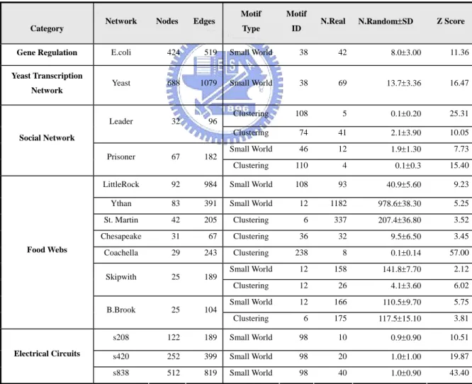
In food webs (Table 2), we found that, skipwith and bridgebrook both have small-world three chain and clustering branch motifs. With clustering branch motif, it exhibits that in such food web, there are many preys for the predator to select, once the predator is eliminated, the food web will be seriously affected. If the relation between predator and prey is removed, it will not affect food web too much, since there are still many other preys for predator to eat. On the other hand, the small-world three chain shows that there are few preys for the predator. Once

these prey or the relation between predator and prey, are removed, it will result a seriously consequence for the food web, not only the possibility of extinction of the prey, but it may lead to a disequilibrium of the whole food web if this relation between predator and prey is a role like bridge. Since relation plays important roles in the food webs, thus protection of these motifs is also an important issue. However, Milo’s method cannot differentiate one’s function from another’s.

Category Network Nodes Edges

Motif Type

Motif

ID N.Real N.Random±SD Z Score Gene Regulation E.coli 424 519 Small World 38 42 8.0±3.00 11.36 Yeast Transcription

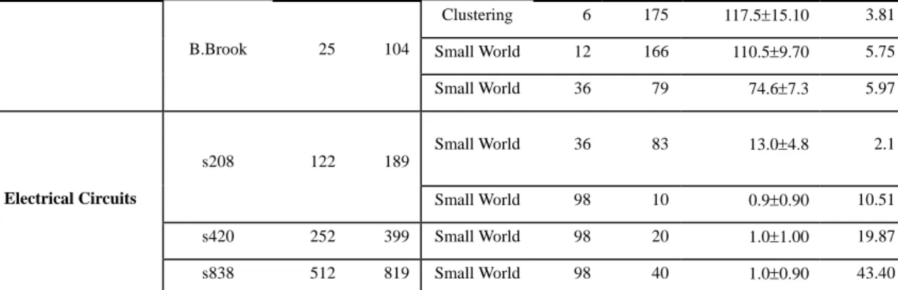
Network Yeast 688 1079 Small World 38 69 13.7±3.36 16.47 Clustering 108 5 0.1±0.20 25.31 Leader 32 96 Clustering 74 41 2.1±3.90 10.05 Small World 46 12 1.9±1.30 7.73 Social Network Prisoner 67 182 Clustering 110 4 0.1±0.3 15.40 LittleRock 92 984 Small World 108 93 40.9±5.60 9.23 Ythan 83 391 Small World 12 1182 978.6±38.30 5.25 St. Martin 42 205 Clustering 6 337 207.4±36.80 3.52 Chesapeake 31 67 Clustering 36 32 9.5±6.50 3.45 Coachella 29 243 Clustering 238 8 0.1±0.14 57.00 Small World 12 158 141.8±7.70 2.12 Skipwith 25 189 Clustering 12 26 4.1±3.60 6.02 Small World 12 166 110.5±9.70 5.75 Food Webs B.Brook 25 104 Clustering 6 175 117.5±15.10 3.81 s208 122 189 Small World 98 10 0.9±0.90 10.51 s420 252 399 Small World 98 20 1.0±1.00 19.87 Electrical Circuits s838 512 819 Small World 98 40 1.0±0.90 43.40 Table 2. Network motifs found in biologival and technological networks.

4.2 A network with only small-world motifs

We found that only small-world motifs exist in electrical circuit, but no clustering motifs. This is because in electrical circuit designs, engineers commonly try to eliminate redundant circuit for economical cost reasons. Furthermore, signal transmissions between input and output usually are directly transmitted, avoiding any intermediate node that may increase the delay time, and the implementation of this circuit also implies that there may contain more “weak-ties” in the circuit. The more complex and mass the layout of the circuit, the more the delay time. Thus clustering motifs are sparse even absent in the electrical circuit designs. However, small-world motif provides us a plain and low-delay principle in designing circuit.

4.3 A network with only clustering motifs

Most of real networks have small-world motifs. But the experiments results show that none of clustering motif but small-world motif exists in the leaderInter social network and four various food webs. For example, in social network there are clustering combined branches motif whose edges are all strong-ties, in other words, two strangers with a common friend have a higher than average probability of meeting each other and becoming friends themselves. In coachllaInter, we have found ten clustering motifs which represent that this network’s clustering is very significant; This results also implies that because of its various connections, it won't lose its connections to others easily by the noise of the artificial or nature way. Certainly, there may exists some weak-ties in the network, but with the number of them is few, it's not shown particularly only because the quantities are not large. However, this clustering motif shows “the richer becomes much richer”.

4.4 Compare different networks

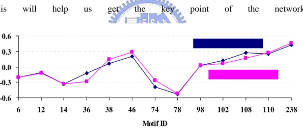
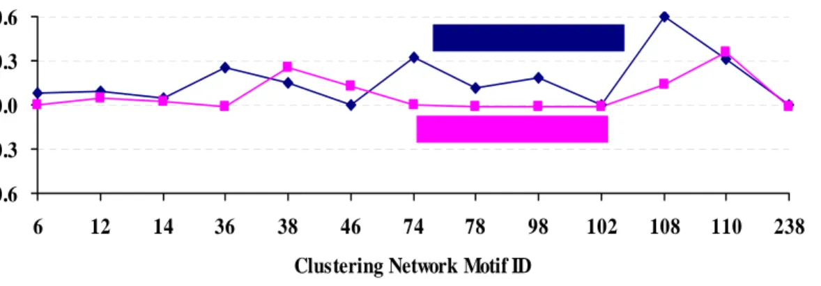
In the previous method (2), leaderInter and prisonerInter of Social networks are classified as similar networks, with the correlation coefficient of 0.962(Figure 4), but in our experimental results, it shows differences from before, we noticed that leaderInter has more remarkable small-world motifs (small-world correlation coefficient = 0.746) (Figure 5), specially small-world uplinked mutual dyad motif, and it shows that many nodding acquaintances in this network. Whereas prisonerInter has more clustering motif (clustering correlation coefficient = 0.311) (Figure 6), especially combined branch motif, since there are more tightly connected groups in this network. When we are grouping real networks by small-world motif or clustering motif, we not only classify them based on their local structure, but also on their global information. This will help us get the key point of the network.

-0.6 -0.3 0.0 0.3 0.6 6 12 14 36 38 46 74 78 98 102 108 110 238 Motif ID

Figure 4. The curve of the normalized Z score thorough Milo’s motif

-0.6 -0.3 0.0 0.3 0.6 6 12 14 36 38 46 74 78 98 102 108 110 238

Small-World Network Motif ID

Figure 5. The curve of the normalized Z_SmallWorld Score through small-world motif and classification

-0.6 -0.3 0.0 0.3 0.6 6 12 14 36 38 46 74 78 98 102 108 110 238

Clustering Network Motif ID

Figure 6. The curve of the normalized Z_Clustering Score through clustering motif and classification

4.5 Explore the details of each complex network

5 Conclusion

In the previous researches about complex networks, we have observed the small-world property in real networks, such as biological, sociological, and technological networks. We find the functional motifs which can represent more global information after giving the weak or strong properties of edge to the Milo’s motif. We can suitably master the design principle of the real complex networks. This is a great help for understanding the real complex networks in the future for everyone. By using our methods, we can compare different networks in proper way instead of too big or too small view.

We provided a general definition for the edge’s weight and weak-tie connection, and it is suitable for any complex network. For a specific field of science, it can define the edge’s weight and weak-tie connection by itself to match its special meaning, and the remainder part can use the method we mentioned in this paper which has generality and extensibility.

We have already found out the motifs that are statistically significant and functionally important in the network, and tried to use these motifs to explain “the behavior of the process” in the network. However, we cannot make sure the thing that is whether or not there are other important factors which affect the network or if the motif we have found out is the most important factor affecting network. We did not have a theoretical framework to confirm us if we are in a right place. Second, there is much to be done in developing more sophisticated models of networks, both to help us understand network topology and to act as a substrate for the study of processes taking place on networks. While some network

causes and effects well understood, others such as correlations, transitivity, and community structure have not [3]. We believe these factors affecting the behavior and the response of the network. For this sake, the future work of this paper is to rebuild networks [24]. The reason why we want to rebuild networks is:

1.) It is hard to collect the complete data, such as: citation networks or sexual relationship network.

2.) The amount of the original data is too large to collect, such as: www. Third, the ultimate goal of the study of the complex networks is to understand the behavior and function of the networked systems [22] [23]. For instance, to explain how the topology of the World Wide Web affects Web surfing and search engines, how the structure of a food web affects population dynamics, and so forth [3].

Reference

1. Buchanan, M., Nexus: Small worlds and the groundbreaking science of networks.

2. Milgram, S., The Small-World Problem. Psychology Today, 1967. 1: p. 60-67.

3. Newman, M.E.J., The Structure and Function of Complex Networks. 2003. 4. Strogatz, D.J.W.a.S.H., Collective Dynamics of 'Small-world' Networks.

Nature. Nature, 1998. 393(6684): p. 440-442.

5. Dorogovtsev, S.N., Mendes, J. F. F., and Samukhin, A. N., Size-dependent degree distribution of a scale-free growing network. Phys, 2001. Rev.: p. E 63.

6. R. Milo, S.S.-O., S. Itzkovitz, N. Kashtan, D. Chklovskii, and U. Alon, Network Motifs: Simple Building Blocks of Complex Networks. Science, 2002. 298: p. 824-827.

7. Artzy-Randrup Y, F.S., Ben-Tal N, Stone L., Comment on "Network Motifs: Simple Building Blocks of Complex Networks" and "Superfamilies of Evolved and Designed Networks". Science, 2004.

8. Granovetter, M.S., The Strength of Weak Ties: A Network Theory Revisited. Sociological Theory, 1983. 1: p. 203-233.

9. Chen, X.F.W.a.G., Complex Networks: Small-World, Scale-Free and Beyond. IEEE Circuits and Systems Magazine, 2003. First Quarter: p. 6-20.

10. R. Milo, S.I., N. Kashtan, R. Levitt, S. Shen-Orr, I. Ayzenshtat, M. Sheffer, and U. Alon, Superfamilies of Evolved and Designed Networks. Science, 2004. 303: p. 1538-1542.

11. S. Shen-Orr, R.M., S. Mangan and U. Alon, Network motifs in the transcriptional regulation network of Escherichia coli. Nature Genetics, 2002. 31: p. 64-68.

12. A.Downing, D.T.a.J., Biodiversity and Stability in Grasslands. Nature, 1991. 367: p. 363-365.

13. R. Kannan, P.T., S. Vempala, Random Struct. Algorithm, 1999. 14: p. 293. 14. M. Newman, G.B., Monte Carlo Methods in Statistical Physics. 1999.

15. al., H.S.e., RegulonDB (version 3.2): transcriptional regulation and operon organization in Escherichia Coli K-12. Nucleic Acids Res, 2001. 29: p. 72-74.

16. al., T.S.e., Nucleic Acids Res, 2002. 29: p. 75-79. 17. Macrae, Sociometry, 1960. 23: p. 360-371. 18. Zeleny, L.D., Sociometry, 1950. 13: p. 314-328. 19. R.Williams, N.M., Nature, 2000. 404: p. 180.

20. Lun Li, D.A., Walter Willinger and John Doyle, A First-Principles Approach to Understanding the Internet's Router-level Topology. ACM SIGCOMM, 2004. 34(4): p. 3-14.

21. Vogt, H., Small Worlds and the Security of Ubiquitous Computing. IEEE CS, 2005.

22. Hui Zhang, A.G., Ramesh Govindan, Using the Small-World Model to Improve Freenet Performance. IEEE Infocom, 2002.

23. Hongsuda Tangmunarunkit, R.G., Sugih Jamin, Scott Shenker, Network Topology Generators: Degree-Based vs. Structural. ACM SIGCOMM, 2002: p. 37.

6 附錄 A

Generation of Random Network

Milo 使用了兩種演算法來確保隨機網路和真實的網路的每個點能有相同的 in-degree 和 out-degree， 這兩種所得到的結果是一樣的。

演算法 A：採用了 Markov-chain 演算法[13]，先造一個和真實網路一樣的隨 機網路，在隨機的挑選一對連結做交換(X1->Y1, X2->Y2 變成 X1->Y2, X2->Y1 假如 X1->Y2 或 X2->Y1 不存在的話)一直到整個隨機網路的亂度夠大為止。 演算法 B：修改[14]的方法，和演算法 A 中一樣，不允許任兩點間有超過一 條的連線。每一個網路以連結矩陣 M 來表示，Mij=1 假如從 node i 到 node j 有 一條連結存在的話，否則 Mij=0。這是為了要讓隨機網路的 Mrand和真實網路的 Mreal 在 欄 和 列 上 有 相 同 的 非 零 數 目 。 Ri=

∑

∑

∑

∑

∑

∑

，假若 Mrand,nm=0，M rand,mn=1，而 Rm=Rm-1，Cn=Cn-1。假如 M rand,mn=1

或 m=n，我們就選擇新的一個(m,n)，一直重複這個步驟直到 Ri=0 和 Cj=0。

Controlling for Appearances of (n-1)-Node Motifs

在我們所產生隨機網路中，每一個都和真實網路有相同的數目的(n-1)node subgraph，這樣的 null hypothesis 是為了在尋找 3-node 的基調時，能夠不受 substructure 的影響太大。我們的作法如了如上所說保持每個點的 in-degree 和 out-degree 不變外，我們也保持了每個點的 mutual edge(XÅÆY)的數目。我們使 用上述的演算法 A，分別處理 double edge 和 single edge 的情形，一個 double edge 只 可 以 和 另 一 個 double edge 做 交 換 (X1ÅÆY1, X2ÅÆY2 to X1ÅÆY2, X2ÅÆY1)假若(X1 和 Y2)(X2 和 Y1)在任何一個方向都是沒有連結的話。同樣

的，有方向性的 single edge 改變連結(X1ÆY1, X2ÆY2 變成 X1ÆY2, X2ÆY1) 只有在改變連結後不會形成 double edge 的情形下。

Network Motif Detection

在 一 個 連 結 矩 陣 M 為 了 要 有 效 率 的 計 算 所 有 有 連 結 的 n-node subgraph，尋找基調的演算法會將所有的列都掃過一遍。對於每一個非零的矩陣 元素(i,j)，再看其他的元素(i,k)(k,i)(j,k)(k,j)一直到所有的 n-node subgraph 都看過 後。Size=3 的每一種 subgraph 在網路中出現的次數都會被紀錄在一個表格中， 並且將所有不同 M 但是外表形狀是相同的 subgraph 加在一起。在每一個隨機網 路中，這一個步驟一直重複直到每一個非零的矩陣元素(i,j)都有找過一遍為止， 並且記錄每一種的 subgraph 出現的次數以和真實網路中出現的次數做比較。

Compare among different Networks

對於每一個 subgraph i，其統計上的重要性以 Z score 來表示：

) ( _i i i i Nrand std Nrand Nreal Z = −

Nreali 代表 subgraph i 出現在真實網路中的次數， Nrand 和 STD(Nreali i)

分別代表 subgraph i 在隨機網路中出現次數的平均值和標準差。而 SPi則是將 Z score 做長度為 1 的正規化後的值： 2 1 2 ) (

∑

附錄 B

Directed Network Description

Gene regulation Directed transcriptional regulation between operons[15] Yeast transcription Directed transcriptional regulation between genes[16]

Social Network Inmates in prison choose “What fellows on the tier are you closest friends with? [17]”.

College students in a course about leadership choose which three members they wanted to have in a committee [18].

Food webs Tropic interactions in ecological food webs[19]

Electrical circuits The nodes represent logic gates and flip-flops. These data parsed from ISCAS89 benchmark set

附錄Ｃ

Category Network Nodes Edges Motif Type

Motif

ID N.Real N.Random±SD Z Score Gene Regulation E.coli 424 519 Small World 38 42 8.0±3.00 11.36

Small World 38 69 13.7±3.36 16.47 Yeast Transcription

Network Yeast 688 1079 _{Clustering 6 41 0.4±1.0 45.06}

Clustering 6 11 3.0±3.1 25.31 Clustering 12 25 6.9±6.5 2.79 Clustering 36 72 8.3±7.9 8.04 Clustering 38 3 0.3±0.6 4.61 Clustering 74 41 2.1±3.90 10.05 Leader 32 96 Clustering 108 5 0.1±0.20 25.31 Clustering 12 33 15.6±8.5 2.07 Clustering 38 8 0.5±0.7 10.6 Small World 46 12 1.9±1.30 7.73 Small World 108 6 1.1±1.2 4.43 Small World 110 8 2.0±1.2 5.04 Social Network Prisoner 67 182 Clustering 110 4 0.1±0.3 15.40 Small World 46 296 221.3±16.7 4.49 LittleRock 92 984 Small World 108 93 40.9±5.60 9.23 Ythan 83 391 Small World 12 1182 978.6±38.30 5.25 St. Martin 42 205 Clustering 6 337 207.4±36.80 3.52 Chesapeake 31 67 Clustering 36 32 9.5±6.50 3.45 Clustering 6 287 169.8±21.8 5.41 Clustering 12 129 28.8±8.4 11.88 Clustering 36 201 95.0±12.3 8.66 Clustering 38 306 103.6±15.1 12.8 Clustering 46 58 4.8±1.9 28.3 Clustering 74 61 5.9±3.1 17.89 Clustering 108 31 10.2±2.1 10.27 Clustering 110 7 0.3±0.6 11.5 Coachella 29 243 Clustering 238 8 0.1±0.14 57.00 Clustering 6 325 185.1±28.1 4.98 Small World 12 158 141.8±7.70 2.12 Clustering 12 26 4.1±3.60 6.02 Clustering 38 106 36.5±23.0 3 Small World 46 45 40.1±0.6 2.6 Food Webs Skipwith 25 189 Clustering 108 15 9.6±1.6 3.45

Clustering 6 175 117.5±15.10 3.81 Small World 12 166 110.5±9.70 5.75 B.Brook 25 104 Small World 36 79 74.6±7.3 5.97 Small World 36 83 13.0±4.8 2.1 s208 122 189 Small World 98 10 0.9±0.90 10.51 s420 252 399 Small World 98 20 1.0±1.00 19.87 Electrical Circuits s838 512 819 Small World 98 40 1.0±0.90 43.40 Table 4. The details of the motifs in each network

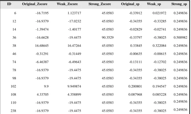
在 Gene Regulation(coliInterFullVec1.txt)，Yeast Transcription Network(yeast.txt) 中都有 small-world motif 的存在(Table 4)，我們發現其實是因為不管是 gene 或是 operon 中的相互的反應都很少會有群聚性的性質存在，也就是說不會同時有很多 個 gene 或多個 operon 和一個 gene 或 operon 有反應，因為 gene 或 operon 通常 都是有他們自己獨特的功能，只能和某些特定的對象反應。他們的角色就像橋樑 一樣，當這些 gene 或 operon 被移除時，可能會因為找不到可代替的而產生極大 的影響。關於 yeast.txt 的測試資料的詳細結果在 Table5 中，id 是指 motif 的 id， 共有 13 種。而我們用之前 Milo 所得的 Zscore 標示為 original_Zscore，之後我們 的方法將 motif 分成兩個 small-world motif 和 clustering motif 所得的 Zscore 分別 標為 weak_Zscore 及 strong_Zscore，而我們將 original_Zscore，weak_Zscore 和 strong_Zscore 分別正規化成為長度 1 後所得值就是 original_sp，weak_sp 和 strong_sp。我們由 Figure 7 可以很明顯的看出在原有的方法其找到的大多數是屬 於 small-world motif。這也說明了我們的方法是更具區辨性的。

ID Original_Zscore Weak_Zscore Strong_Zscore Original_sp Weak_sp Strong_sp 6 -16.7195 1.123717 45.0583 -0.33912 0.021972 0.249836 12 -16.9379 -17.0232 45.0583 -0.34355 -0.33285 0.249836 14 -1.39474 -1.40177 45.0583 -0.02829 -0.02741 0.249836 36 -16.6628 -19.4475 90.3529 -0.33797 -0.38025 0.500982 38 16.68645 16.47264 45.0583 0.33845 0.322084 0.249836 46 -0.31291 -0.31449 45.0583 -0.00635 -0.00615 0.249836 74 -6.46387 -6.49643 45.0583 -0.13111 -0.12702 0.249836 78 -16.9379 -19.4475 45.0583 -0.34355 -0.38025 0.249836 98 -16.9379 -19.4475 45.0583 -0.34355 -0.38025 0.249836 102 9.9 9.949874 45.0583 0.200801 0.194547 0.249836 108 4.33705 4.358899 45.0583 0.087968 0.085228 0.249836 110 -16.9379 -19.4475 45.0583 -0.34355 -0.38025 0.249836 238 -16.9379 -19.4475 45.0583 -0.34355 -0.38025 0.249836

Table 5. Yeast 的 Zscore 和 Superfamily

-0.6 -0.4 -0.2 0 0.2 0.4 0.6 6 12 14 36 38 46 74 78 98 102 108 110 238 original_sp weak_sp strong_sp

Figure 7. Yeast 的 Superfamily

在 Social Network 中，我們針對兩類的網路來討論。第一類是 Leader 的網路，我們發現在其網路中都是群聚性基調，因為在裡面大部分的人（都是 leader）都會找其同好，甚至組成小團體，並且在這種網路中，因為競爭較為明 顯，較不易有如君子的點頭之交存在，也因此其小世界基調在裡面也就不明顯(當

然也是存在一定的比例，如 Table 6，Figure8 所示）。第二類是 prisoner 的網路， 我們發現裡面除了有群聚性基調外，也有小世界基調(如 Table 7，Figure9 所示)。 在監獄中無可避免的一定會有小團體存在，可能就是被關在一起的幾個人就組成 了一個小團體，並且在裡面也會機會出現點頭之交的朋友，可能大家是在一起吃 飯的時候，或是放風的時間，就彼此認識了。

ID Original_Zscore Weak_Zscore Strong_Zscore Original_sp Weak_sp Strong_sp 6 -1.747412 -3.287122 2.590444 -0.20969 -0.22023 0.082448 12 -0.937555 -3.019262 2.793733 -0.11251 -0.20228 0.088918 14 -2.793824 -3.255373 1.364124 -0.33526 -0.2181 0.043417 36 -1.044121 -8.133933 8.044244 -0.1253 -0.54495 0.256029 38 0.566814 -0.46433 4.607804 0.068019 -0.03111 0.146656 46 1.663396 1.678409 -0.100504 0.199611 0.112448 -0.0032 74 -3.253861 -9.626284 10.045202 -0.39047 -0.64493 0.319715 78 -4.387757 -5.168297 3.451602 -0.52654 -0.34626 0.109856 98 0.217539 -0.621614 5.686241 0.026105 -0.04165 0.18098 102 1.045186 1.048487 -0.100504 0.125424 0.070245 -0.0032 108 2.310234 -0.735767 25.311394 0.277233 -0.04929 0.805602 110 2.076463 1.174308 9.949874 0.24918 0.078675 0.316681 238 3.591276 -0.540117 -0.10054 0.43096 -0.03619 -0.0032

Table 6. Leader 的 Zscore 和 Superfamily

-1 -0.5 0 0.5 1 6 12 14 36 38 46 74 78 98 102 108 110 238 original_sp weak_sp strong_sp

ID Original_Zscore Weak_Zscore Strong_Zscore Original_sp Weak_sp Strong_sp 6 -6.31005 -1.28729 -0.16873 -0.20119 -0.08592 -0.00396 12 -3.7163 -3.1816 2.079942 -0.11849 -0.21236 0.048762 14 -10.3395 -4.52546 1.128846 -0.32966 -0.30205 0.026465 36 -8.88971 -1.83048 -0.73229 -0.28344 -0.12218 -0.01717 38 4.680244 0.649788 10.59812 0.149223 0.04337 0.248461 46 8.831725 7.730779 5.249851 0.281587 0.515996 0.123077 74 -8.07271 -4.37754 -0.07007 -0.25739 -0.29218 -0.00164 78 -16.3888 -7.72919 -0.68034 -0.52253 -0.51589 -0.01595 98 0.755017 0.758821 -0.732294 0.024073 0.050648 -0.01717 102 1.86011 1.991263 -0.27435 0.059307 0.132908 -0.00643 108 5.152789 4.431013 5.686241 0.164289 0.295751 0.133308 110 8.502822 5.044127 15.40288 0.2711 0.336673 0.361104 238 14.40838 -0.38685 -0.732294 0.459391 -0.02582 -0.01717

Table 7. Prisoner 的 Zscore 和 Superfamily

-0.6 -0.4 -0.2 0 0.2 0.4 0.6 6 12 14 36 38 46 74 78 98 102 108 110 238 original_sp weak_sp strong_sp

Figure 9. Prisoner 的 Superfamily

在我們探討的七個食物鏈中，我們也發現一些有趣的現象。在 St. Martin， Chesspeake 和 coachellaInter 中都只有存在群聚性基調(如 Table 8，Table9， Table 10 和 Table 11 所示)，我們覺得在這三個地方的生態是較屬於一種”動態的穩定 [12]---即網路越複雜，波動就越小，比單純的網路更為穩定”，在這三種食物鏈 網路中，群聚性基調扮演了維持生態平衡的一個很重要的角色。假設某一種掠食

者有十五種獵物，如果其中有一種變的很少時，掠食者對其自然不是趕盡殺絕， 而是轉移注意力到其他物種，畢竟其他的十四種獵物數量較多，也比較容易取 得。這種注意力的轉移，讓掠食者仍可以找到食物，而那個有滅絕危險的獵物也 得以休養生息。這樣一來，食物鏈中因為群聚性基調化解了危險的波動，他可說 是生態係中的天然壓力閥。

ID Original_Zscore Weak_Zscore Strong_Zscore Original_sp Weak_sp Strong_sp 6 5.021437 2.349219 -1.43135 0.344815 0.137488 -0.11347 12 6.656267 5.246372 -1.41398 0.457077 0.307045 -0.1121 14 -0.29792 0.077245 -0.65099 -0.02046 0.004521 -0.05161 36 5.046043 0.851961 -1.46478 0.346505 0.049861 -0.11612 38 -5.15904 -2.76497 -1.41697 -0.35426 -0.16182 -0.11233 46 1.180611 1.592555 -0.41082 0.081071 0.093204 -0.03257 74 -0.76969 0.332168 -0.70142 -0.05285 0.01944 -0.05561 78 -5.15904 -2.76497 -1.46478 -0.35426 -0.16182 -0.11612 98 -2.13993 -2.28712 -0.14286 -0.14695 -0.13385 -0.01133 102 -1.47295 -1.75495 -0.26149 -0.10115 -0.10271 -0.02073 108 1.342258 1.205492 -0.71322 0.092171 0.070552 -0.05654 110 -5.15904 -2.76497 -1.46478 -0.35426 -0.16182 -0.11612 238 -5.15904 -2.76497 -1.46478 -0.35426 -0.16182 -0.11612

Table 8. Ythan 的 Zscore 和 Superfamily

-1 -0.5 0 0.5 1 6 12 14 36 38 46 74 78 98 102 108 110 238 original_sp weak_sp strong_sp

ID Original_Zscore Weak_Zscore Strong_Zscore Original_sp Weak_sp Strong_sp 6 -0.85325 -3.73667 3.522563 -0.10304 -0.3176 0.779525 12 1.77455 -0.63137 1.93752 0.214302 -0.05366 0.428763 14 -2.65069 -3.73667 0.31449 -0.32011 -0.3176 0.069595 36 -0.85325 -2.17196 1.834843 -0.10304 -0.18461 0.406041 38 0.853245 0.701046 0.029506 0.103041 0.059586 0.00653 46 -2.65069 -3.73667 -0.31449 -0.32011 -0.3176 -0.0696 74 -2.65069 -3.73667 -0.31449 -0.32011 -0.3176 -0.0696 78 -2.65069 -3.73667 -0.31449 -0.32011 -0.3176 -0.0696 98 -2.65069 -2.67395 -0.31449 -0.32011 -0.22727 -0.06959 102 -2.65069 -3.73667 -0.31449 -0.32011 -0.3176 -0.0696 108 -2.65069 -3.73667 -0.31449 -0.32011 -0.3176 -0.0696 110 -2.65069 -3.73667 -0.31449 -0.32011 -0.3176 -0.0696 238 -2.65069 -3.73667 -0.31449 -0.32011 -0.3176 -0.0696

Table 9. St. Martin 的 Zscore 和 Superfamily

-0.4 -0.2 0 0.2 0.4 0.6 0.8 1 6 12 14 36 38 46 74 78 98 102 108 110 238 original_sp weak_sp strong_sp

ID Original_Zscore Weak_Zscore Strong_Zscore Original_sp Weak_sp Strong_sp 6 -1.71691 -2.87112 1.661523 -0.29547 -0.22051 0.380712 12 -0.36932 -1.20247 1.63356 -0.06356 -0.09235 0.374305 14 -1.71691 -4.15513 -0.41082 -0.29548 -0.31913 -0.09413 36 -1.71691 -4.15513 3.45395 -0.29547 -0.31913 0.791419 38 1.716908 1.799664 -0.41082 0.295475 0.13822 -0.09413 46 -1.71691 -4.15513 -0.41082 -0.29548 -0.31913 -0.09413 74 -1.71691 -4.15513 -0.41082 -0.29548 -0.31913 -0.09413 78 -1.71691 -4.15513 -0.41082 -0.29548 -0.31913 -0.09413 98 -1.09635 -1.10187 -0.41082 -0.18868 -0.08463 -0.09413 102 -1.71691 -4.15513 -0.41082 -0.29548 -0.31913 -0.09413 108 -1.71691 -4.15513 -0.41082 -0.29548 -0.31913 -0.09413 110 -1.71691 -4.15513 -0.41082 -0.29548 -0.31913 -0.09413 238 -1.71691 -4.15513 -0.41082 -0.29548 -0.31913 -0.09413

Table 10. Chesspeake 的 Zscore 和 Superfamily

-0.4 -0.2 0 0.2 0.4 0.6 0.8 1 6 12 14 36 38 46 74 78 98 102 108 110 238 original_sp weak_sp strong_sp

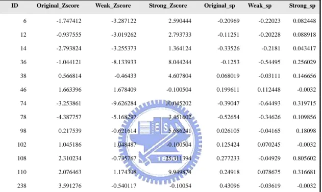
ID Original_Zscore Weak_Zscore Strong_Zscore Original_sp Weak_sp Strong_sp 6 -3.54714 -6.67046 5.405872 -0.26303 -0.29937 0.076242 12 3.930769 -4.53703 11.87985 0.291477 -0.20362 0.167549 14 -5.67502 -6.33327 2.342074 -0.42082 -0.28424 0.033032 36 -5.0119 -11.9216 8.662428 -0.37165 -0.53505 0.122171 38 2.087713 -10.2013 12.81541 0.15481 -0.45784 0.180743 46 6.16401 -4.37193 28.31973 0.457078 -0.19621 0.39941 74 -1.85739 -8.96517 17.88596 -0.13773 -0.40236 0.252256 78 -2.87256 -2.87137 -0.47826 -0.21301 -0.12887 -0.00675 98 -3.32883 -3.27169 -0.41082 -0.24684 -0.14684 -0.00579 102 -3.77928 -3.50148 -1.59456 -0.28024 -0.15715 -0.02249 108 3.486546 -0.65457 10.27412 0.258537 -0.02938 0.144902 110 0.305105 -1.2277 11.49675 0.022624 -0.0551 0.162146 238 2.199358 -3.52769 57.00582 0.163088 -0.15832 0.803987

Table 11. coachellaInter 的 Zscore 和 Superfamily

-1 -0.5 0 0.5 1 6 12 14 36 38 46 74 78 98 102 108 110 238 original_sp weak_sp strong_sp

Figure 13. CoachellaInter 的 Superfamily

反觀在 LittleRock，或是 B.Brook 這兩種小世界基調較多的食物鏈網路， 我們覺得他們是較不”穩定”的(如 Table 11，Table12 所示)。在小世界基調中，只 要有一個物種數量減少了，很快的就會使的相關的物種受到影響，因為他們較具 有不可替代性，可能一個物種滅亡了，而他又是扮演一個橋樑的角色，如此就會 使的生態系中的食物鏈出現斷層，其影響是非常大的。

ID Original_Zscore Weak_Zscore Strong_Zscore Original_sp Weak_sp Strong_sp 6 -3.16468 0.461409 -0.75495 -0.19604 0.03128 -0.35 12 1.941243 1.337675 -0.78232 0.120252 0.090684 -0.36269 14 -4.54282 -3.37524 -0.57256 -0.28141 -0.22882 -0.26544 36 -3.47632 0.123292 -0.7745 -0.21534 0.008358 -0.35907 38 2.432854 1.399384 -0.84311 0.150706 0.094868 -0.39087 46 5.023007 4.486077 -0.47983 0.311155 0.304122 -0.22245 74 -7.61981 -6.9357 -0.54746 -0.47202 -0.47019 -0.25381 78 -1.38492 -1.38319 -0.20412 -0.08579 -0.09377 -0.09463 98 -6.02156 -6.05151 -0.37256 -0.37301 -0.41025 -0.17272 102 -2.55845 -2.55461 -0.36786 -0.15849 -0.17318 -0.17054 108 9.238748 9.235317 -0.50509 0.572303 0.626085 -0.23417 110 -0.67044 -0.66601 -0.14286 -0.04153 -0.04515 -0.06623 238 1.773848 1.788265 -0.84311 0.109883 0.121231 -0.39087

Table 12. LittleRock 的 Zscore 和 Superfamily

-1 -0.5 0 0.5 1 6 12 14 36 38 46 74 78 98 102 108 110 238 original_sp weak_sp strong_sp

ID Original_Zscore Weak_Zscore Strong_Zscore Original_sp Weak_sp Strong_sp 6 4.584513 -1.84006 3.808106 0.305372 -0.1979 0.50422 12 7.312807 5.747983 -1.17603 0.487103 0.61819 -0.15571 14 -0.98171 -0.41356 -0.48082 -0.06539 -0.04448 -0.06366 36 4.856907 -1.75855 5.979292 0.323516 -0.18913 0.791701 38 -5.16754 -3.62932 0.61633 -0.34421 -0.39033 0.081606 46 1.512368 1.749745 -0.32962 0.100738 0.188183 -0.04364 74 -2.08256 -1.87271 -0.42268 -0.13872 -0.20141 -0.05597 78 -5.16754 -2.17544 -1.17603 -0.34421 -0.23397 -0.15571 98 -2.16441 -2.17544 -0.3386 -0.14417 -0.23397 -0.04483 102 -1.22636 -1.22657 -0.1005 -0.08169 -0.13192 -0.01331 108 2.59057 2.56718 -0.48044 0.172557 0.276098 -0.06361 110 -5.16754 -2.17544 -1.17603 -0.34421 -0.23397 -0.15571 230 -5.16754 -2.17544 -1.17603 -0.34421 -0.23397 -0.15571

Table 13. B. Brook 的 Zscore 和 Superfamily

-0.5 0 0.5 1 6 12 14 36 38 46 74 78 98 102 108 110 238 original_sp weak_sp strong_sp Figure 15. B. Brook 的 Superfamily

在食物鏈網路 skipwith 中，其同時具有顯著的小世界基調和群聚性基調(如 Table 14 所示)。我們覺得這種生態在遭受外界的干擾時，會因為他的群聚性基調 而維持整個生態的平衡，但同時又因為在此生態中沒有許多的 hub(存在群聚性基 調中的)，也就是和許多生物有關係的生物存在，不容易因受外界的干擾而導致 整個生態嚴重的瓦解。

ID Original_Zscore Weak_Zscore Strong_Zscore Original_sp Weak_sp Strong_sp 6 1.166676 -4.97063 4.981989 0.12233 -0.40178 0.581827 12 5.754029 2.121066 6.016856 0.603328 0.17145 0.702685 14 -1.52663 -1.52221 -0.1005 -0.16007 -0.12304 -0.01174 36 1.304625 1.857087 -0.76268 0.136794 0.150112 -0.08907 38 -1.88959 -3.15688 2.960739 -0.19813 -0.25518 0.345773 46 2.782947 2.600902 -0.1005 0.291801 0.210236 -0.01174 74 -2.41688 -2.41517 -0.1005 -0.25342 -0.19522 -0.01174 78 -2.17163 -4.97063 -0.76268 -0.2277 -0.40178 -0.08907 98 -2.15961 -2.17049 -0.76268 -0.22644 -0.17544 -0.08907 102 -2.17163 -2.18257 -0.76268 -0.2277 -0.17642 -0.08907 108 3.430743 3.452393 -0.1005 0.359724 0.279063 -0.01174 110 -2.17163 -4.97063 -0.76268 -0.2277 -0.40178 -0.08907 238 -2.17163 -4.97063 -0.76268 -0.2277 -0.40178 -0.08907

Table 14. Skipwith 的 Zscore 和 Superfamily

-0.5 0 0.5 1 6 12 14 36 38 46 74 78 98 102 108 110 238 original_sp weak_sp strong_sp

Figure 16. SkipwithInter 的 Superfamily

最後我們討論在 Electrical Circuits 中的兩個網路，我們發現他們之中都 沒有群聚性基調的存在，而只有小世界基調的存在。而會造成這種現象的原因正 如在本文中所探討的三個原因之外，我們也發現的確在電路中，”feedback”的架 構扮演了一個重要的角色(如 Table 15，Table 16 和 Table 17 所示)。在電路中，最 常見的 feedback 架構就如 Figure 17 所示：

Figure 17. General Feedback Structure

以 negative feedback 為例，其所具有得五個特性是：1) Desensitized gain 2)Reduce nonlinear gain 3) Reduce effects of noise 4)Control input and output impedances 5)Extend bandwidth of amplifier。在電路設計的運用上，feedback 的基 調的確佔了一個重要的地位。

ID Original_Zscore Weak_Zscore Strong_Zscore Original_sp Weak_sp Strong_sp 6 1.714808 0.424154 -0.1673 0.060871 0.035817 -0.03529 12 -8.65087 -0.57413 -1.43396 -0.30708 -0.04848 -0.30252 14 -8.65087 -1.66292 -1.50147 -0.30708 -0.14042 -0.31677 36 1.714808 2.104422 -1.50147 0.060871 0.177704 -0.31677 38 -1.71481 -1.66292 -0.30151 -0.06087 -0.14042 -0.06361 46 -8.65087 -1.66292 -1.50147 -0.30708 -0.14042 -0.31677 74 -8.65087 -1.66292 -1.50147 -0.30708 -0.14042 -0.31677 78 -8.65087 -1.66292 -1.50147 -0.30708 -0.14042 -0.31677 98 10.54809 10.50778 -0.14286 0.374427 0.887312 -0.03014 102 -8.65087 -1.66292 -1.50147 -0.30708 -0.14042 -0.31677 108 -8.65087 -1.66292 -1.50147 -0.30708 -0.14042 -0.31677 110 -8.65087 -1.66292 -1.50147 -0.30708 -0.14042 -0.31677 238 -8.65087 -1.66292 -1.50147 -0.30708 -0.14042 -0.31677

-0.4 -0.2 0 0.2 0.4 0.6 0.8 1 6 12 14 36 38 46 74 78 98 102 108 110 238 original_sp weak_sp strong_sp Figure 18. S208 的 Superfamily

ID Original_Zscore Weak_Zscore Strong_Zscore Original_sp Weak_sp Strong_sp 6 1.788484 0.451044 -0.35737 0.03538 0.086732 -0.06841 12 -15.5247 -1.45449 -1.7031 -0.30711 -0.75287 -0.32601 14 -15.5247 -1.72251 -1.7031 -0.30711 -0.75287 -0.32601 36 1.788484 1.208996 -0.94222 0.03538 0.086732 -0.18036 38 -1.78848 -1.72251 -0.37363 -0.03538 -0.08673 -0.07152 46 -15.5247 -1.72251 -1.7031 -0.30711 -0.75287 -0.32601 74 -15.5247 -1.72251 -1.7031 -0.30711 -0.75287 -0.32601 78 -15.5247 -1.72251 -1.7031 -0.30711 -0.75287 -0.32601 98 19.40711 19.86786 -0.17586 0.383913 0.941144 -0.03366 102 -15.5247 -1.72251 -1.7031 -0.30711 -0.75287 -0.32601 108 -15.5247 -1.72251 -1.7031 -0.30711 -0.75287 -0.32601 110 -15.5247 -1.72251 -1.7031 -0.30711 -0.75287 -0.32601 238 -15.5247 -1.72251 -1.7031 -0.30711 -0.75287 -0.32601

-1 -0.5 0 0.5 1 1.5 6 12 14 36 38 46 74 78 98 102 108 110 238 original_sp weak_sp strong_sp Figure 19. S420 的 Superfamily

ID Original_Zscore Weak_Zscore Strong_Zscore Original_sp Weak_sp Strong_sp 6 1.903386 0.941179 -0.86316 0.017566 0.021366 -0.12968 12 -33.1911 -2.3996 -2.16197 -0.30631 -0.05447 -0.32481 14 -33.1911 -2.3996 -2.16197 -0.30631 -0.05447 -0.32481 36 1.903386 1.395896 -1.11214 0.017566 0.031688 -0.16708 38 -1.90339 -1.75915 -0.48432 -0.01757 -0.03993 -0.07276 46 -33.1911 -2.3996 -2.16197 -0.30631 -0.05447 -0.32481 74 -33.1911 -2.3996 -2.16197 -0.30631 -0.05447 -0.32481 78 -33.1911 -2.3996 -2.16197 -0.30631 -0.05447 -0.32481 98 42.60697 43.39078 -0.14286 0.393212 0.985007 -0.02146 102 -33.1911 -2.3996 -2.16197 -0.30631 -0.05447 -0.32481 108 -33.1911 -2.3996 -2.16197 -0.30631 -0.05447 -0.32481 110 -33.1911 -2.3996 -2.16197 -0.30631 -0.05447 -0.32481 238 -33.1911 -2.3996 -2.16197 -0.30631 -0.05447 -0.32481

Table 17. S838 的 Zscore 和 Superfamily

-0.5 0 0.5 1 1.5 6 12 14 36 38 46 74 78 98 102 108 110 238 original_sp weak_sp strong_sp Figure 20. S838 的 Superfamily