Multiple soliton interactions in a polarization-division multiplexing system

Ž . Optics Communications 147 1998 42–46

Multiple soliton interactions

in a polarization–division multiplexing system

Sien Chi

, Chi-Feng Chen, Jeng-Cherng Dung

Institute of Electro-Optical Engineering, National Chiao Tung UniÕersity, 30050 Hsinchu, Taiwan, ROC Received 8 July 1997; revised 17 September 1997; accepted 30 September 1997

Abstract

We numerically study multiple soliton interactions in a polarization–division multiplexing transmission system. It is found that, unlike the transmission system of solitons with the same polarization, the two soliton interaction is not the strongest compared to the interaction of more than two solitons. Therefore, the maximum transmission distance limited by the interaction of solitons cannot be inferred by the collision distance of two solitons in a polarization–division multiplexing system and the interactions of more solitons must be considered. q 1998 Elsevier Science B.V.

1. Introduction

The interaction of solitons is an important limitation of the bit rate–distance product in a soliton transmission system. The experiments demonstrated that the interaction between orthogonally polarized solitons is weaker than

w x

that of parallel polarized solitons 1,2 . Therefore, a way to reduce the soliton interactions and increase transmission capacity is to make the adjacent soliton orthogonally polar-ized, which is called the polarization–division

multiplex-Ž . w x

ing PDM technique 1–6 . Moreover, whenever two or-thogonal polarized solitons at the input of a fiber transmis-sion link may maintain a high degree of polarization throughout the whole link, even though the presence of random variations of fiber birefringence and polarization

w x

dispersion 1 . In fact, it is considered that the typical length scale where birefringence and polarization disper-sion fluctuations occur is much shorter that the soliton period, so that the fluctuating local birefringence vector

w x

may be averaged over all polarization states 7,8 . The soliton interaction in a PDM system has been analyzed by

)

E-mail: [email protected].

w x

the perturbation method 3–5 . On the other hand, to reduce the soliton–soliton interaction and noise-induced timing jitter in parallel polarized soliton transmission sys-tem, an the optical bandpass filter with frequency sliding is

w x

inserted after every optical amplifier 9–11 . In recent experimental and theoretical works, it has been found that the interaction between PDM solitons is also notably

re-Ž . w x

duced by a sliding-frequency filter SFF 2,5 .

In a parallel polarized soliton transmission system, the distance of soliton coalescence which is based on the interaction between two solitons is a good indication of the maximum transmission distance since two soliton interac-tion is stronger than more than two soliton interacinterac-tions

w x

which have longer coalescence distance 12 . So far, for a PDM soliton transmission system, only two soliton

interac-w x

tion has been analyzed theoretically 3–5 , where the maximum transmission distance of a PDM soliton system is considered by the coalescence distance of two solitons. In this paper, we numerically analyze the interactions among multiple solitons in a PDM system. It is found that the interaction between two solitons is no longer the main limitation factor for a PDM transmission system. In the considered cases, the distance of coalescence of two soli-tons is shortest for four soliton interaction. If we use the SFF in the PDM system, the soliton interaction becomes 0030-4018r98r$19.00 q 1998 Elsevier Science B.V. All rights reserved.

Ž . PII S 0 0 3 0 - 4 0 1 8 9 7 0 0 5 8 0 - 4

weaker. In this case the two soliton interaction is weaker than more than two solitons. Therefore, the maximum transmission distance cannot be inferred by the coales-cence distance of two solitons, and we must consider the interactions of more than two solitons.

2. Theory

The PDM soliton propagation in a random birefringent fiber can be described by the coupled averaged

propaga-Ž . w x

tion equations CAPE 7,8

Ž . Ž . Ž .

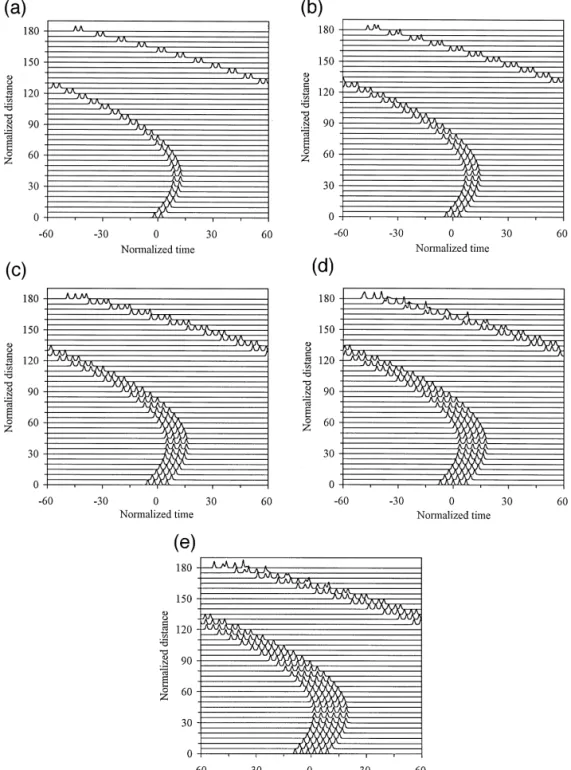
Fig. 1. Mutual interactions of multiple solitons in a PDM transmission system: a two soliton interaction, b three soliton interaction, c

Ž . Ž .

Eu 1 E2u _{2 2} < < < < i q q

_Ž

_.

_Ž

_.

Ž

.

Ž

.

'

'

where u s 9r8 U, Õ s 9r8 V. U and V are the two polarization components of the electric field envelope nor-malized by the electric field scale Q, Z and T are normal-ized by the dispersion length L , and time scale T ,_{D 0} respectively. Q, LD and T are related by0

1r2 2 < < l b₂ A_eff T₀ Q s ₂ , L s_D , <b < 2p n T2 0 2

where l is the wavelength, b₂ is the group-velocity dispersion parameter, Aeff is the effective fiber cross section, and n is the Kerr coefficient, T s T r1.763 and_{2 0 W}

TW is the full pulsewidth at half magnitude. g s a LD

where a is the fiber loss. For a PDM soliton system, the polarizations of the neighboring solitons are orthogonal. On the other hand, the parallel polarized soliton

propaga-Ž .

tion in a single mode fiber can be described by Eq. 1a without Õ component.

The transfer function of the optical filter placed after every amplifier is taken as

1

H V y V

Ž

.

Ž .

1 q i 2rB

_Ž

_.

_Ž

_.

where V s v y v₀ and v₀ is the original soliton carrier frequency, V is the center frequency of the filter, and Bf

is the filter bandwidth. For the SFF, in dimensionless units, V s a Z where af 0 0 is the sliding rate.

3. Numerical solutions and discussion

Ž .

We use the split-step Fourier method to solve Eqs. 1 . The fiber loss is periodically compensated by the lumped amplifiers and the amplification period is assumed to be 0.25L . The normalized filter bandwidth is taken to beD

B s 9. To show multiple soliton interactions, we take a 3.5

pulse width separation between neighboring solitons to enhance the interaction. In the following discussion, the distance is normalized by L_D and the time is normalized by T . We have numerically simulated the propagation ofW

multiple solitons in a parallel polarized soliton transmis-sion system, the behaviors are similar to those shown in

w x

Ref. 12 . The two solitons coalesce at about 17L ,_D whereas, the other multiple solitons interact after this coalescence distance. Thus, the interaction between two solitons is the main limitation in a parallel polarized soliton transmission system. In Fig. 1, we show the mutual interactions of multiple solitons in a PDM soliton

transmis-< transmis-<2

sion system. Figs. 1a–1e show the power envelope u q

< <2

Õ of two solitons, three solitons, four solitons, five

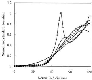
solitons, and six solitons, respectively. In Fig. 1a, two solitons attract each other and collide at about 112 L . For_D a larger number of solitons, the two outside solitons are repulsed at about 37L . It is seen from Figs. 1 that in the_D case of four solitons the two pulses in the center coalesce at a distance of 75L , and for the other cases the center_D solitons collide after this coalescence distance. The aver-age standard deviations of the timing jitter of the solitons only caused by the soliton interactions are shown in Fig. 2. The average standard deviations of the timing jitter are calculated by the following process. We assume that there are N pulses and their initial positions are written to be

P , P , . . . , P_{01 02 0 N}. First, we find the pulse positions P ,_i1

P , . . . , Pi2 i N at some propagation distance, they are written too. Then we obtain D P s P y P_{i j i j 0 j} where

j s 1, . . . , N. Finally, we can obtain the average

stand-a r d d e v i a t i o n s o f t h e t i m i n g j i t t e r ,

2

D P s Ý D P y ÝD P

(

_Ž

_.

i j i j i j

the case of two solitons the standard deviation gradually increases until the collision distance, and in the cases of larger number of solitons initially the pulses maintain their relative positions, then the standard deviations greatly increase after the distance 50 L . The standard deviation of_D the four solitons is larger than that of the other cases after the distance 59LD and is found to be maximum at about 75L_D where the center solitons coalesce. Therefore, the maximum transmission distance can not be inferred by the collision of two solitons in a PDM soliton transmission system.

In Fig. 3, we show the mutual interactions of multiple solitons in a PDM soliton transmission system with frequency filters. Here, we use a

up-sliding-Fig. 2. Evolutions of the standard deviations of the timing jitters

Ž .

of the solitons for different soliton interaction. Two

Ž . Ž .

soliton interaction, –)– three soliton interaction, –(– four

Ž . Ž .

soliton interaction, –^– five soliton interaction, and –q– six soliton interaction.

frequency filter with a normalized sliding rate of 0.03 to

w x

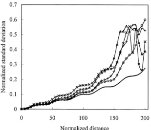
reduce the soliton interaction 9 . It can be seen from Fig. 3 that the solitons maintain well up to 180 L_D for the two solitons case, but for the other cases the solitons collide before that distance. In the considered cases, the coales-cence distance of five solitons is the shortest, about 160 L .D

Fig. 4 shows the standard deviations of the solitons

consid-ered in Fig. 3. One can be see that the standard deviation of the two solitons is smaller than that of more than two solitons. Therefore, the allowed transmission distance for a PDM transmission system should be much shorter than the distance expected from the interaction of two solitons in a communication system.

For a numerical example in terms of real units, we take

Fig. 4. Same as in Fig. 2, with up-sliding-frequency filters.

2

Ž

T_Ws12 ps and b s y0.382 ps rkm₂ D s 0.3

.

psrkmrnm . When sliding-frequency filters are not used, the isolated two adjacent solitons collide at about 13.5 Mm, and in the case of four solitons the two central pulses coalesce at a distance of about 9 Mm. When up-sliding-frequency filters are used, the shortest coalescence distance found in the case of four solitons is about 19.4 Mm.

4. Conclusion

In conclusion, we numerically study the interactions of multiple solitons in a PDM transmission system. It is found that, unlike the parallel polarized soliton transmis-sion system, the two soliton interaction is not the strongest compared to the interaction of more than two solitons. In fact, when sliding-frequency-filters are used in a PDM

system, the two soliton interaction has the least standard deviation of timing jitters. Therefore, the maximum trans-mission distance limited by the interaction of solitons can not be inferred by the collision distance of two solitons in a PDM system, and the interactions of more solitons must be considered.

Acknowledgements

This work is partially supported by the National Sci-ence Council, Republic of China, under Contract NSC 86-2811-E009-002R.

References

w x_{1 S.G. Evangelides, L.F. Mollenauer, J.P. Gordon, N.S.}

Ž .

Bergano, J. Lightwave Technol. 10 1992 28.

w x_{2 L.F. Mollenauer, P.V. Mamyshev, M.J. Neubelt, Optics Lett.}

Ž .

19 1994 704.

w x_{3 C. De Angelis, S. Wabnitz, M. Haelterman, Electron. Lett.}

Ž .

29 1993 1568.

w x4 C. De Angelis, S. Wabnitz, Optics Comm. 125 1996 186.Ž . w x5 S. Wabnitz, Optics Lett. 20 1995 261.Ž .

w x_{6 F. Matera, M. Romagnoli, B. Daino, Electron. Lett. 31} Ž1995 1172..

w x_{7 P.K.A. Wai, C.R. Menyuk, H.H. Chen, Optics Lett. 16} Ž1991 1231..

w x_{8 P.K.A. Wai, C.R. Menyuk, H.H. Chen, Optics Lett. 16} Ž1991 1735..

w x_{9 L.F. Mollenauer, J.P. Gordon, S.G. Evangelides, Optics Lett.}

Ž .

17 1992 1575.

w10 Y. Kodama, S. Wabnitz, Optics Lett. 18 1993 1311.x Ž . w11 Y. Kodama, S. Wabnitz, Optics Lett. 19 1994 162.x Ž . w12 J.R. Taylor Ed. , Optical Solitons – Theory and Experiment,x Ž .