Received September 15, 1997; revised May 14, 1998; accepted August 20, 1998. Communicated by Jieh Hsiang.
1 A CPM/PERT can be either an AOV or an equivalent AOA (Activity On Arc) network. Here, AOV is adapted for comparison with SPREM.
2 Here, deterministic means that when a process on vertex V is complete, then all of Vs successors will enact the process individually.
423
Short Paper
A Project Model for Software Development
BIN-SHIANG LIANG, JENN-NAN CHEN*AND FENG-JIAN WANGInstitute of Computer Science and Information Engineering National Chiao Tung University
Hsinchu, Taiwan 300, R.O.C. E-mail: fjwang@csie.nctu.edu.tw
*Samar Techtronics Cooperation Ltd.
Taiwan, R.O.C.
Uncertainty and dynamic changes in a software project cause iterations during development and the need for decision-making in planning and controlling a project. This paper presents a Software Project Review and Evaluation Model, SPREM, a superset of CPM/PERT, which extends CPM/PERTs notation to four types of verti-ces (AA, AX, XA, and XX vertiverti-ces) to express the non-deterministic and iterative behaviors of software engineering projects. Several behavioral properties of SPREM and analysis of them are discussed. For example, the enaction capability can be used to evaluate the possibility that a vertex will enact processes beforehand. Project managers can revise a SPREM graph to rescue dead vertices before project execution. Furthermore, enaction ordering allows project managers to calculate the dependency between processes to be enacted. This might help in computing important informa-tion such as critical paths among these processes.
Keywords: CPM/PERT, software project management, SPREM, software process modeling, project evaluation
1. INTRODUCTION
The CPM (Critical Path Method)/PERT (Plan Evaluation and Review Technique) net-work has been applied broadly to project management. It is an acyclic and directed AOV (Activity On Vertex)1 network able to express sequential, parallel, and synchronous activity
behaviors [3, 20]. However, its deterministic2 and acyclic properties are not suitable for
managing projects consisting of iteratively and decisionally-based procedures [20]. Especially, it is not suitable for software development, due to the lack of iteration and decision-making [5, 7, 20, 23]. Many studies have been devoted to extending CPM/PERT to modeling of the behaviors of projects with a high degree of uncertainty and dynamically changing
characteristics. These studies can be divided into two categories: one category extends the different types of CPM/PERT network vertices [9, 10, 12, 27], and the other combines CPM/ PERT with Petri nets [20, 21, 25]. GANs (Generalized Activities Networks) [12] introduces a simple dichotomous choice at each vertex in order to provide a decision-box planning and scheduling technique for research projects.
GAN, devised in [10], views vertices from input and output logic perspectives. Unfortunately, these papers seem unclear in their definition [9]. GERT (Graphical Evalua-tion and Review Technique) is based on ideas introduced in [27] and adds notaEvalua-tions con-cerning Exclusive-OR (XOR) vertices and the probability of OR/XOR vertices existing in the network. Clearly, this method is restricted by analysis limitations, and its analysis relies only on simulations. Design/Net [20] combines AND-OR graphs with Petri net notation to describe and monitor software processes. However, it is acyclic, and little analysis is provided. [25] combined Beat-distributed stochastic Petri nets with PERT, and [21] com-bined generalized stochastic Petri nets with PERT for performance evaluation of concur-rent processes. Both have problems with computational complexity in exploring state spaces during analysis, and currently must restrict nets to being acyclic to reduce the computa-tional complexity. In summary, the former category is limited to reliance on simulation [9]. As for the latter, evaluating the performance of Petri nets even with deterministic timing and firing frequencies per cycle for all state transitions is often an NP-hard problem [29]. Furthermore, this approach seems unsuitable for managing large and complicated projects because Petri nets use lower-level semantics for comprehension.
This paper presents the Software Project Evaluation and Review Model (SPREM), a superset of CPM/PERT that extends CPM/PERTs notation to four types of vertices (AA, AX, XA, and XX vertices). SPREM can express the various behaviors required to model software engineering projects. A* (AX and AX) vertices are able to model the syn-chronization of a process while *A (AA and XA) vertices can model the fork of parallel processes. X* (XA and XX) vertices are able to model what-if processes while *X (AX and XX) vertices model decision-making processes. Looping is allowed in SPREM so as to model iterative processes. With SPREM, managers can model large and complicated projects using top-down and/or bottom-up approaches since a vertex can be decomposed into a SPREM graph containing a set of vertices. Also, analysis in SPREM, such as enaction capability and performance analysis, can be computed with a reasonable cost. Enaction capability analysis can be used to evaluate the potential of a vertex to enact processes beforehand. Project managers can revise a SPREM graph to rescue dead vertices before project execution. In addition, enaction ordering allows project managers to calculate the dependency between the processes to be enacted. This might help in computing important information, such as critical paths among these processes.
The rest of this paper is organized as follows. Section 2 defines SPREM and dis-cusses its enaction behaviors. To demonstrate the modeling ability of SPREM, section 3 presents an example based on the spiral model paradigm [4], widely accepted as a realistic software development paradigm. The example indicates that with SPREM, it is easier to model a software project than it is with a Petri net. In section 4, some interesting charac-teristics of SPREM are defined and discussed. Sections 5 and 6 present the analysis algo-rithms of SPREM, which are of interest during project planning and are introduced at two levels, acyclic and cyclic, respectively. Some conclusions and future work are described in section 7.
2. A SPREM GRAPH
2.1 Definition of SPREM
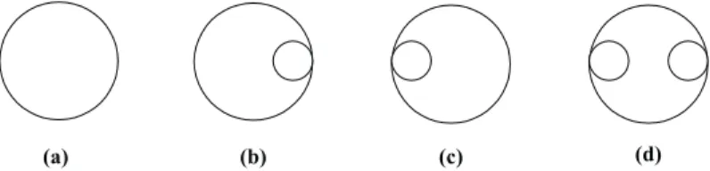
A SPREM graph is a Five-tuple <V, A, Sp, Ep, M0>. V = {V1, V2, ..., Vm} is a finite set of
vertices, where m, m ≥ 0, is the number of vertices. There are four types of vertices: AA (AND-AND), AX (AND-XOR), XA (XOR-(AND-AND), and XX (XOR-XOR), where A represents all, X represents exclusion, and the first character represents the condition that enacts the ver-tex process while the second represents what is to be done at the end of the process. Fig. 1 (a-d) shows the notation associated with AA, AX, XA, and XX vertices, respectively.
Fig. 1. The notation associated with four types of vertices in SPREM.
A: V ¥ V = {A1, A2, ..., An} is a finite set of directed arcs, where n, n ≥ 0, is the number
of arcs. Each arc is associated with a Boolean value. Each pair of vertices contains at most one directed arc. If a vertex contains only an input arc, the vertex is both an A* vertex and an X* vertex. When a SPREM graph contains only AA vertices and no loops, the graph is a CPM/PERT network.
Sp, Ep: There is only one entry vertex called Start Project, Sp, and only one exit
vertex called End Project, Ep, in any SPREM graph. To simplify discussion, Sp has no
input, and Ep has no output arcs.
M0: A Æ B is an initial SPREM graph indicating where B is a set of Boolean values.
A vertex is enactable if its precondition holds; i.e., the value of its input arc(s) satis-fies an AND or XOR condition. An A* vertex is enactable when all its input arcs are set to TRUE. An X* vertex is enactable when one of its input arcs is set to TRUE and the rest are FALSE.
The Boolean values of arcs are assigned initially and then set or reset by its tail or head during execution. The precondition of all vertices cannot hold at the beginning; i.e., only vertex Sp can enact a process at the beginning.
A vertex enacts a process once, including instantiating, running, and then terminating the process. To simplify discussion, we assume that there is no condition checking, arc value changing, or time consumption for process instantiation/termination. Every input arc of an enabled vertex is set to FALSE while the vertex is instantiating a process. A process starts to run as soon as it is instantiated. A vertex is active when it has a process running. An enactable vertex cannot enact a new process if it is active; that is, a vertex cannot enact a new process when it has a process running even though value changes in its input arc(s) make it enactable. After the running process has been terminated, the vertex enacts a new process if it is enactable. The values of the vertex output arcs can be treated as contribu-tions for the termination of processes associated with the vertex. When *A vertex V
termi-nates its process, it sets all Vs output arcs to TRUE. When *X vertex V termitermi-nates its process, it sets one of Vs output arcs to TRUE and the rest to FALSE, no matter what their values were previously.
A vertex in a SPREM graph can represent another SPREM graph. For vertex Va
rep-resenting SPREM graph SPa, instantiating for Va means instantiating Sp in SPa. If the
pro-cess in Va runs, this means that the vertices in SPa except for Sp, run processes. The design
of SPa is erroneous, if Ep cannot enact a process. Ep in SPa may enact more than one
process. SPa is considered complete only when no running processes exist in any vertices
of SPa. The process in Va is terminated when SPa finishes (due to enaction).
Obviously, a SPREM graph may allow a vertex to enact more than one process even though it contains no loop. For example, let X* vertex V contain only two predecessors, which are enacting two distinct processes pa and pb, where pa terminates earlier than pb.
Assume that the process enacted by V terminates between the termination of pa and pb. V
will enact one new process when process pb is terminated. In other words, V enacts two
processes.
3. AN EXAMPLE OF MODELING A SPIRAL MODEL
To demonstrate the modeling ability of SPREM, an example based on the spiral model paradigm [4] is presented in this section. This paradigm for software engineering is one realistic approach to the development of large-scale software systems [26]. The paradigm defines four major phases to be iterated evolutionarily during each development cycle: (1) planning determination of objectives, alternatives, and constraints, (2) risk analysis -analysis of alternatives and identification/resolution of risks, (3) engineering - develop-ment of the next-level product, and (4) customer evaluation - assessdevelop-ment of the results of engineering. Obviously, the CPM/PERT technique fails to model this paradigm naturally. 3.1 A SPREM Example
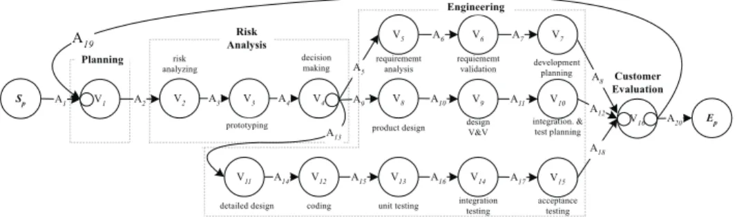
When a development process is modeled using SPREM, its referred/generated arti-facts can be modeled as the attributes associated with the input/output arcs of a vertex. The artifacts must remain at some state and are changed after a process is enacted. Also, infor-mation and/or states of resources and staffs can be modeled as vertex attributes to express the requirements needed to enact processes. Fig. 2 shows the paradigm modeled using SPREM. The processes/artifacts along each vertex/arc in Fig. 2 are listed in (Appendix) Table 5 and Table 6, respectively. Fig. 10 in the Appendix shows the state transition dia-gram of a software artifact manipulated by processes.
In Fig. 2, the paradigm is modeled as an iterative cycle identified as A19 (the LBA)
incident from V16 to V1 and containing four phases. Each phase is shown within the region
enclosed by a dashed line. The planning phase contains V1 only to express the process
determine-objectives-alternatives-and-constraints. Assume that the project is required to produce a product called artifact software. Software stays in an initialized state at the beginning, described as A1. After the planning phase software is translated into a planned
state, described as A2, the project enters the risk-analysis phase, which contains V2, V3, and
V4. V2 enacts the risk-analysis process to analyze alternatives and identify/resolve risks.
After risks have been analyzed, described as A3, a prototype of software is produced,
de-scribed as A4, by the process prototyping enacted by V3.
Each time a prototype is generated and simulated (or measured), the decision-mak-ing process on V4 (an AX vertex) will choose one thread in the engineering phase to enact
processes. For example, enacting process product-design on vertex V8 requires that artifact
product-design-specification be initialized or modified, i.e., requires A9 to be TRUE. The
Engineering phase contains three threads: requirement analysis, product design, and de-tailed design. Each time one thread is chosen and executed, a process in the customer-evaluation phase is followed to plan the next-level product and assess the results of engi-neering software. For example, if the product design phase is chosen, then the process product-design on V8 translates artifact product-design-specification from the initial or
modi-fied state to the completed state. After the process verification-and-validation on V9 is
completed, the process integration-and-test-plan on V10 and the process
customer-evalua-tion on V16 (an XX vertex) are enacted.
At the end of a development cycle, the process customer-evaluation on V16 either
chooses (1) an iterate cycle, described as A19 (software = evaluated) or (2) terminates the
project, described as A20 (software = completed).
Fig. 10 in the Appendix shows softwares state transition diagram derived from the example in Fig. 2. The state transition diagram provides managers with a product view so that they can monitor and control projects. A product view gives the current state of a product, which reveals the completeness of the product. SPREM can present various views in multiple layers, where a higher-layered view can hide the details of the lower ones. For example, software can be considered as the super-artifact of the artifacts requirement-specification, product-design-requirement-specification, detailed-design-requirement-specification, and module. Each sub-artifact has its own state transition diagram. In this case, if software transits from the prototype-created state to the integration-tested state, this means that the artifacts detailed-design-specification and model have been completed.
3.2 A Short Comparison
Petri nets are successful in a wide variety of applications. They have been extended with different notations for different applications, especially timing and functional modeling. Timing is mainly concerned with performance evaluation, including evaluation of the Time Petri Net (TPN) [24], Timed Petri Net, (TdPN) [28], Stochastic Petri Net (SPN) [22] etc.
The functional capability is used to describe various functional specifications of a system. This category of high-level Petri nets includes the Colored Petri Net (CPN) [17], Predicate/ Transition net (Pr/T net) [15], Entity/Relation net (ER net) [16] etc. These nets have some similarities and allow tokens to carry various kinds of information.
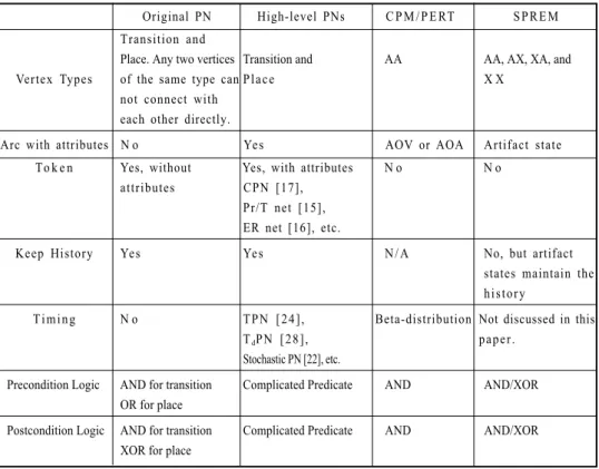
Some comparisons between SPREM and Petri nets are summarized in Table 1 based on an example Petri net for modeling of the spiral paradigm, shown in Fig. 3.
Table 1. Summary of comparisons between SPREM and Petri Nets.
Original PN High-level PNs C P M / P E RT SPREM Transition and
Place. Any two vertices Transition and AA AA, AX, XA, and
Vertex Types of the same type can Place X X
not connect with each other directly.
Arc with attributes N o Yes AOV or AOA Artifact state
To k e n Yes, without Yes, with attributes N o N o attributes CPN [17],
Pr/T net [15], ER net [16], etc.
Keep History Yes Yes N/A No, but artifact
states maintain the history
Timing N o TPN [24], Beta-distribution Not discussed in this
TdPN [28], paper.
Stochastic PN [22], etc.
Precondition Logic AND for transition Complicated Predicate AND AND/XOR OR for place
Postcondition Logic AND for transition Complicated Predicate AND AND/XOR XOR for place
Fig. 3. An example of modeling the spiral model using a Petri Net.
Petri nets have two vertex types, transition and place, while SPREM has four: AA, AX, XA, and XX. In a Petri net, a token is added to a place cumulatively when the process on an input transition of the place finishes. The value of an arc in SPREM is set or reset when a process enaction or completion occurs in its head or tail, respectively, no matter what its current value is. SPREM is suitable for modeling a system which focuses on the current status only, but a Petri net is better for a system that needs to keep history information.
SPREM is more concise than Petri nets. In the example of modeling the spiral model, 16 transitions, 14 places, and 33 arcs are used in the Petri net shown in Fig. 3, but 18 vertices and 20 arcs are used in the SPREM graph shown in Fig. 2.
In SPREM, the logic operators in a precondition/postcondition of a vertex used to enact a process are either AND or XOR. In a Petri net, the logic operator is AND-AND for a transition and OR-XOR for a place. Firing a transition T consumes one token from each of Ts input places and generates one token which is sent to all of Ts output places. For a place P, any of Ps input transitions can generate a token sent to P while a token in P can only be consumed by one of Ps output transitions. The precondition/postcondition for firing a transition can be a complicated predicate in a high-level Petri net. With SPREM, software project managers can get a more natural view from a graph since the pre/ postcondition of enacting a process for a vertex can be seen directly from the SPREM graph.
Furthermore, it is worth noting that SPREM is not intended to serve independently as a software Process Modeling Language PML. Many researches [5, 6, 11, 13] in software process modeling have adopted high-level Petri nets to serve as PMLs. Some comparisons between these PMLs can be found in [1, 14, 23, 31]. To model a software development process, a PML is required to describe various and complicated elements, such as people, resources, artifacts, inter-structures of individual elements, and interrelations between elements, rather than the behavior only [1-3, 8, 9, 14]. SPREM uses simple notation for modeling various behaviors required in software engineering projects such that some man-agement parameters for the projects, such as the enaction capability and schedule, can be evaluated beforehand or during project execution. Also, SPREM is one part of PLAN, a PML used in our related work [18].
4. SOME CHARACTERISTICS OF A SPREM GRAPH
4.1 Enaction Capability
Vertices in a SPREM graph can be divided into four enactability kinds according to their enaction capability. A vertex V is called dead if V cannot enact a process. Vertex V is called simple if V can enact one and only one process. Vertex V is called essential if V can enact at least one process. Vertex V is called dangerous if it is not one of the above; i. e., it is indeterminate.
A vertex and its successors (predecessors) are not necessarily of the same enactability kind. The enactability kind of a vertex can be determined by several factors: its type (A* or X*), its predecessor types, the values of its input arcs, and its execution behavior (process duration or decision-making).
Obviously, an A* vertex is dead if it has one FALSE input arc with a dead tail. An X* vertex is dead if (1) it has two or more TRUE input arcs, either of whose tails are dead or *A; i.e., these arcs cannot be set to FALSE any more by their tails, or (2) all of its input arcs are FALSE with dead tails.
Whether or not a dangerous vertex can enact a process cannot be determined before project execution. For example, an A* vertex V is dangerous if it has one not-dead prede-cessor whose type is *X and may always set its output arc to V to FALSE; i.e., V can not enact any processes. An X* vertex is dangerous if it has two or more TRUE input arcs among which there exists at most one whose tail is dead or *A.
Let a vertex V have m input arcs Aj, j = 1, 2, ..., m, and let each Aj have tail Vj. Suppose
vertex Vj enacts processes no more than MaxEN(Vj) times and no less than MinEN(Vj)
times.
Consider the case in which V is A*. V enacts at least one process if each of Vs input arcs Aj satisfies one of the following cases: (1) Aj is TRUE and has a *A tail, (2) Aj is TRUE
and has a dead* *X tail, or (3) Aj is FALSE and has a simple or essential *A tail. The
maximum number of processes enacted by V is MaxEN V MaxEN V
j m j
( )=min ( )+
≤ ≤
1 dj, where dj is equal to one when Aj is TRUE, zero
otherwise. (1)
The minimum number of processes enacted by V is
MinEN V MinEN V
j m j j
( )=min min ( )+ ,
1≤ ≤ δ 1, if all of Vs processors are *A. (2)
Consider the case in which V is X*. The maximum number of processes enacted by V is
MaxEN V
MaxEN V V s ar TRUE
MaxEN V k V has k TRUE k
j j m j j m ( ) ( ), ; ( ) , , . = ∑ − + ∑ ≥ ≤ ≤ ≤ ≤
if at most one of in put arcs or
max if in put arcs;
' 1
1
2 0 2
(3) Consider an X* vertex V with all FALSE input arcs. If V has one simple or essential *A predecessor Vj, then Vs enactability kind is the same as that of Vj. If V has two or more
simple or essential *A predecessors, then V is essential. 4.2 Enaction Ordering
A vertex in a SPREM graph is said to depend on another vertex graphically if there exists a path from the latter to the former. A vertex V1 is absolutely dependent on another
vertex V2 if every path from Sp to V2 always contains V1. A vertex V2 absolutely trails
another vertex V1 if every path from V1 to Ep always contains V2.
In a SPREM graph, two vertices have no graphical dependency relationship if there is no path between them. Processes enacted in two distinct vertices may run concurrently, and the order of process enaction in separate vertices is not decided only by their graphical dependency. Thus, it is overly complex and unnecessary to compute the order of enaction in separate vertices. To simplify discussion, here, we consider only the first process enaction in a vertex.
Let the first-enaction of a vertex be the first time the vertex is enacted. A vertex is enaction-prior (enaction-posterior) to another if its first-enaction is earlier (later) than that of the other. A vertex is prior to its A* successor; i.e., an A* vertex is enaction-posterior to its predecessor. A vertex is enaction-prior to its X* successor if there is only one successor. If a vertex is absolutely dependent on another vertex, the latter is always enaction-prior to the former.
The enaction of Sp in a SPREM graph results from an external enaction at the beginning.
During the enaction, Sp does not allow any other external enaction until no vertices in the
SPREM graph contain running processes. A vertex containing no input paths from Sp is not
graphically dependent on Sp. A vertex containing no output paths to Ep is not graphically
depended upon Ep. Two vertices V1 and V2, where V2 is graphically dependent upon V1, do
not necessarily entail V2 enacting a process when V1 does so. Neither does it mean that V1
must enact or complete its process before V2 can enact its process. However, a vertex that
does not depend on Sp graphically can never enact any processes (i.e., it is a dead vertex). A
process of a vertex that Ep does not graphically depend on will not affect the project.
4.3 Looping in a SPREM Graph
A loop is a simple path in which the first and last vertices are the same. Two paths are said to be distinct if they contain no common vertex. A vertex within a loop is called an entry vertex to the loop if there is a path from Sp to the vertex that is distinct from the loop
except for the vertex. A vertex within a loop is called an exit vertex from the loop if there is a path from the vertex to Ep that is distinct from the loop except for the vertex. An input
(output) arc of an entry (exit) vertex of a loop is called an entry (exit) arc of the loop if the arc is not in the loop. A loop may have multiple entry/exit vertices and arcs.
To simplify discussion, each loop in a SPREM graph is allowed to have only one entry vertex, only one exit vertex, and one arc from the exit vertex to the entry vertex of the loop, called the loop back arc (LBA for short). LBAs are initially set to FALSE. A loop can never make the entry A* vertex of the loop enact any process because one input arc (the LBA) is FALSE. A running loop cannot stop if the exit vertex of the loop is *A because the LBA will make the entry X* vertex enact a process when the exit vertex process is terminated. Thus, the entry and exit vertices of a loop must be X* and *X, respectively.
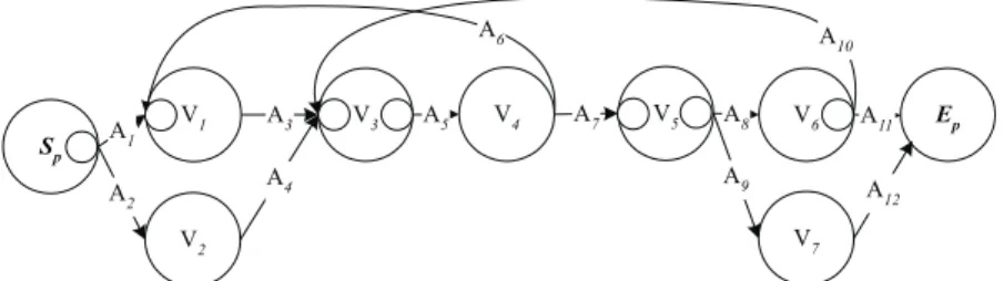
A SPREM graph is well-structured if and only if all the loop(s) in the SPREM graph contain one X* entry vertex, one *X exit vertex, and one FALSE LBA. More than one loop may share a common LBA. In a well-structured SPREM graph, a set of loops sharing a common LBA constitutes a strongly connected subgraph, called an LSUB. An LSUB can be considered as an XX vertex. Thus, a well-structured SPREM graph can be considered as a partially ordered network, where the duration of the associated project can be estimated beforehand. Like unrestricted gotos in programs, general cases of looping are too com-plicated to deal with [30]. A well-structured SPREM graph is more modularized because every LSUB has only one entry and one exit point. The SPREM graph shown in Fig. 4 is not well-structured since the loop (V1, A3, V3, A5, V4, A6, V1) has two entry vertices, V1 and V2,
and the loop (V3, A5, V4, A7, V5, A8, V6, A10, V3) has two exit vertices, V6 and V7.
4.4. Mutual Exclusion and Dependency
A set of vertices is a Mutually Exclusive Set, MES, if the set has more than one vertex, if only one vertex can enact a process, and if no other enaction is possible. The vertices in an MES are called mutually exclusive with respect to enaction. In other words, two vertices are mutually exclusive if they are in a common MES. A Dependent Enaction Set, DES, is a set of vertices in which at least one vertex cannot enact a process.
In an MES of two vertices, when one vertex enacts a process, the other cannot. Con-sider the examples shown in Fig. 5. V1 and V2 in (a) are mutually exclusive since V can
change one output arcs value once. Cases (b-d) are different. For example, in case (d), V1
and V2 enact processes concurrently while A0 and A2 are set to TRUE by V0 and V,
respectively.
Fig. 5. Examples of mutual exclusion.
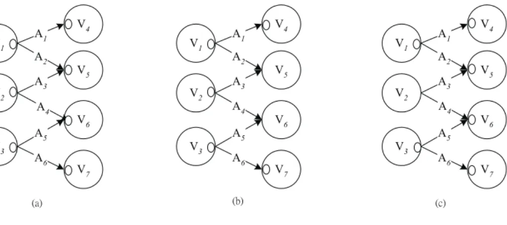
Consider the examples shown in Fig. 6. Let all vertices be simple and all arcs be FALSE. Suppose the set of vertices {V1, V2, V3} is not a DES. Then, the set of vertices S = {V4, V5, V6,
V7} in cases (a) and (b) constitutes a DES, but it does not in case (c). In (a), at most three
vertices in S can enact processes. In (b), only V4, and V6, V4, and V7, or V5 and V7 in S can
enact processes. In (c), all vertices in S can enact processes while A1 is set to TRUE by V1,
A3 and A4 are set to TRUE by V2, and A6 is set to TRUE by V3.
5. ENACTION CAPABILITY OF ACYCLIC SPREM
5.1 Vertex Enactability
Consider a SPREM graph. Let LPN(V)/SPN(V) be the Largest/Smallest Possible Num-ber of processes to be enacted by vertex V. LPN(V) is always larger than or equal to SPN(V). If LPN(V) = 0, V can enact no processes; i.e., V is dead. If LPN(V) = SPN(V) = 1, V can enact one and only one process; i.e., V is simple. If SPN(V) ≥ 1, V can be enact at least one process; i.e., V is essential. If LPN(V) > 0 and SPN(V) = 0, V may or may not enact a process; i.e., V is dangerous. Table 2 summarizes the relationships among the enactability kinds of vertex V and its SPNs and LPNs.
Table 2. Enactability kinds of vertices
LPN(V) =1 LPN(V) =1 LPN(V) >1 SPN(V) = 0 Dead Dangerous Dangerous
SPN(V) =1 X Simple Essential
SPN(V) >1 X X Essential
Let an A* vertex V have m input arcs Aj, j = 1, 2, ..., m and Ajs tail Vj.
V is dead if (1) it has at least one FALSE input arc Aj whose value cannot be changed
to TRUE; i.e., Aj is FALSE and Vj is dead; (2) the set of Vs predecessors whose output arcs
to V are FALSE is a DES; or (3) V is mutually exclusive with one of its predecessor(s) that has a FALSE output arc to V.
V is dangerous (i.e., V may or may not enact a process) if V is not dead and has at least one input arc Aj, and if either (1) Vj is *X and not dead; or (2) Aj is FALSE and Vj is *A
and dangerous. In the former case, Aj may be changed to FALSE before Vs precondition
holds even though it is currently TRUE. In the latter case, Aj may not be changed to TRUE
even when Vj is *A since Vj may not enact a process.
Otherwise, V can enact at least one process (i.e., V is simple or essential) since each input arc Aj is either (1) TRUE and not changed to FALSE by Vj; or (2) FALSE and will be
changed to TRUE. In the former case, Aj is TRUE and Vj is (a) *A, or (b) *X and dead. In
the latter case, Aj is FALSE and Vj is *A and simple or essential.
Let an X* vertex V have m input arcs Aj, j = 1, 2, ..., m and Ajs tail Vj. According to
the value of Vs input arc, V can be classified into one of the following cases: Case 1: V has only one TRUE input arc. This case is not allowed in M0.
Case 2: V has two or more TRUE input arcs. If two or more TRUE input arcs are dead or if *A tails, then V is dead since these arcs can no longer be set to FALSE by their tails. Otherwise, V is dangerous, and the LPN(V) can be obtained from Eq.(3).
Case 3: All of Vs input arcs are FALSE. V is simple or essential if V has at least one simple or essential *A predecessor. V is dead if all of Vs predecessors are dead. Otherwise, V is dangerous since V has at least one dangerous predecessor or one simple or essential *X predecessor. These predecessors will absolutely not change the value of their output arcs to V to TRUE. The LPN(V) of a not-dead vertex can be obtained from Eq.(3). Whether a vertex is simple or essential can be deter-mined as follows:
Case (a): V has one simple or essential *A predecessor Vj. Vs enactability kind is the
same as that of Vj; i.e., SPN(V) = SPN(Vj) and LPN(V) = LPN(Vj).
Case (b): V has two simple or essential *A predecessors, namely Vi and Vj. V is
essential. If SPN(Vi) = 1 and SPN(Vj) = 1, then SPN(V) = 2, SPN(V) = 1
otherwise.
Case (c): V has more than two simple or essential *A predecessors. V is essential and SPN(V) = 1.
5.2 Evaluating an A* Vertex
This subsection discusses how to evaluate the enactability kind of an A* vertex. Given a SPREM graph SP and an A* vertex V in SP, algorithm Evaluate-A-Vertex, presented in Appendix B, can evaluate Vs enactability kind as follows. Let each vertex V in a SPREM graph SP be associated with two integer variables lpn and spn used to store LPN(V) and SPN(V), respectively, and two string variables kind and type to indicate Vs enactability kind and type, respectively. Let each arc A be associated with a Boolean variable value used to store As value and an integer variable isTrue used for computing the lpn and spn of As head. A.isTrue is set to one if A is TRUE, zero otherwise. Before evaluation, in all the vertices and arcs, V.type, A.value, and A. isTrue are defined, and V.kind is set to dead and V. spn and V.lpn are set to zero initially. The evaluation for the A* vertex can be done by following the five steps below.
Step 1: Initialization. In step 1, integer variables MaxEN and MinEN store the results obtained from Eqs.(1) and (2), respectively. The boolean variable VIsDangerous, set to FALSE here, indicates whether V has a predecessor that makes it dangerous. The boolean variable ArcAllTrue, set to TRUE here, indicates whether all input arcs of V are TRUE.
Step 2: Evaluate-A-Vertex uses the function Has-Exclv-Vex() [19] to examine whether V has two predecessors that are mutually exclusive or whether V and one of its predecessor(s) are mutually exclusive. If the result is true, i.e., V is dead, it is returned and the algorithm terminates.
Step 3: Each of Vs predecessors Vj, j = 1, 2, ..., m, is examined as follows. If one
predeces-sor renders V dead, then it is returned and the algorithm terminates. If one prede-cessor renders V dangerous, then VIsDangerous is set to TRUE. If V is found to have has one FALSE input arc, then ArcAllTrue is set to FALSE.
Step 4: ArcAllTrue is checked. If ArcAllTrue = TRUE, then an error is returned since this is not allowed in M0, and the algorithm terminates.
Step 5: VIsDangerous is checked. If VIsDangerous = TRUE, then V.kind is set to dangerous; otherwise, V.kind is set to simple or essential. In step 5.1, V.lpn = MaxENI is set. V.spn = MinEN and V.lpn = MaxEN are set, and V is determined to be simple or essential. If MaxEN =1, i.e., V is simple, then V.kind is set to simple, or to essen-tial otherwise.
Based on the above, algorithm Evaluate-A-Vertex in Appendix B evaluates a vertex Vs enactability kind. It first computes LPN(V)/SPN(V) according to Eqs. (1-2), respectively, when the enactability kind of Vs predecessors are evaluated. Then, it evalu-ates whether V is dead in step 2 (mutual exclusive set checking) and in step 3 (checking whether one predecessor renders V dead), and whether V violates the criteria in M0, in step
4. If these cases do not happen, it determines Vs enactability kind, as discussed in section 5.1, in step 5. Thus, evaluation is correct.
5.3 Evaluating an X* Vertex
This subsection discusses how to evaluate the enactability kind of an X* vertex. Given a SPREM graph SP and an X* vertex V in SP, the algorithm Evaluate-X-Vertex in Appen-dix B can evaluate Vs enactability kind as follows.
Step 1: Initialization. Variables L1 and L2 store the results obtained from Eq.(3). The variables NumOfTrueArc and NumOfPositiveVex, set to zero here, represent the number of Vs TRUE input arcs and simple or essential *A predecessors, respectively. The variable NumOfDead, set to zero here, stands for the number of TRUE input arcs in whose tails are either *A or dead. The variable ExistNeuDanVex, set to FALSE here, indicates whether V has a FALSE input arc whose tail is danger-ous or is simple or essential *X.
Step 2: Each of Vs input arcs Aj and predecessors Vj, j = 1, 2, ..., m is examined. If Aj.value
= TRUE, then (1) NumOfTrueArc is increased by one, and (2) the algorithm checks whether Vj.type = *X or Aj.kind = dead. If the result is TRUE, then NumOfDead is
increased by one. If Aj.value = FALSE and Vj is simple or essential *A, then
NumOfPositiveVex is increased by one. If V is found to have one dangerous or one simple or essential *A predecessor, then ExistNeuDanVex is set to TRUE. Step 3: The algorithm evaluates V in the following cases. In case 1: NumOfTrueArc = 1, it
returns an error since this case is not allowed in M0. In case 2: NumOfTrueArc ≥ 2,
it checks NumOfDead. If NumOfDead ≥ 2, then it returns since V is dead. Otherwise, it sets V.lpn = L1 and V.kind = dangerous. In case 3: NumOfTrueArc = 0. If NumOfPositveVex = 0 and ExistNeuDanVex = TRUE (subcase 1), then V.kind = dangerous and V.lpn = L2 are set (if ExistNeuDanVex = FALSE, then V is dead). If NumOfPositveVex = 1 (subcase 2), then V.spn = Vj.spn and V.kind = Vj.kind are set.
If NumOfPositveVex = 2 (subcase 3), then V.kind = essential is set. If NumOfPositveVex ≥ 3 (otherwise part in subcase), then V.kind = essential and V.spn = 1 are set.
Step 4: The algorithm terminates.
The evaluation correctness for the algorithm Evaluate-X-Vertex is discussed in the following. For a vertex V, let the enactability kind of Vs predecessors be evaluated. The algorithm first computes variables L1 and L2 according to Eq.(3). Then, it computes vari-ables NumOfTrueArc, NumOfDead, NumOfPositiveVex, and ExistNeuDanVex by evaluat-ing each of Vs predecessors in step 2. Based on the above, it correctly determines Vs enactability kind according to these variables.
5.4 Evaluating an Acyclic SPREM
Referring to the discussion in section 5.1, Vs enactability kind can be determined if those of its predecessors are known. A topological sorting algorithm lists the vertices in an acyclic graph with the predecessors at the front. In an acyclic SPREM graph, the algo-rithm Evaluate-Acyclic-SPREM in Appendix B can be used to traverse an acyclic SPREM graph SP to output the LPN, SPN, and enactability kind of each vertex.
Let each vertex V in SP be associated with two integer variables lpn and spn storing LPN(V) and SPN(V), respectively, and two string variables kind and type indicating Vs kind and type, respectively. Let each arc A in SP be associated with a Boolean attribute beenTraversed. The beenTraversed of an arc, set to FALSE initially, is changed to TRUE when its tail is traversed. Let each arc A be associated with a Boolean variable value used to store As value, and an integer variable isTrue used for computing the lpn and spn of As head. A.isTrue is set to one if A is TRUE, zero otherwise.
Evaluate-Acyclic-SPREM uses a queue Q to store vertices temporarily during tra-versal of SP. A vertex V is inserted into Q when all of its input arcs have beenTraversed = TRUE; i.e., the computation of all its predecessor(s) is finished. V is removed from Q while it is being computed. Each vertex can be computed at most once as follows. Step 1: Initialization. Queue Q is cleared. For each vertex V in SP, the variable V.kind is
set to dead, and V.spn and V.lpn are set to zero. For each arc A, A.beenTraversed is set to FALSE, and A.isTrue is set to one if A.value is TRUE, zero otherwise. Step 2: Traversing SP from Sp. First, Sp.kind = simple, LPN(Sp) = 1, and SPN(Sp) = 1 are
set, and beenTraversed in all of the output arcs of Sp is set to TRUE. Then, Sps
successor(s) are inserted into Q if all of their input arcs where beenTraversed = TRUE.
Step 3: Performing traversal with a while loop. The loop is repeated until Q is empty, i.e., until all vertices are traversed. Then the algorithm terminates. In each turn, a vertex V is retrieved from queue Q and evaluated. If V.type = A*, then Evaluate-A-Vertex is invoked, Evaluate-X-Evaluate-A-Vertex otherwise. Then, beenTraversed in all output arcs of V is set to TRUE. If Vs successor has input arcs where beenTraversed = TRUE, then it is inserted into Q.
The algorithm Evaluate-Acyclic-SPREM traverses acyclic SPREM graph SP in topo-logical sorting order using queue Q. This order allows the predecessors of a vertex V to be visited before V; i.e., when V is evaluated, its predecessors have already been evaluated. When V is evaluated, either algorithm Evaluate-A-Vertex or algorithm Evaluate-X-Vertex is used. Thus, evaluation is correct.
5.5 An Example of Evaluating an Acyclic SPREM
A SPREM graph is well-defined if and only if the network contains no dead vertices. Fig. 7 shows a SPREM graph that is not well-defined. Vertex V4 is dead since it has two
TRUE input arcs A4 and A5 whose tails are simple, e.g., V1 and V2, respectively. V8 is
dangerous since it has two TRUE input arcs, A12 and A13, in which A12s tail V5 is *X. Table
3 lists the M0 of the SPREM graph. Table 4 shows the results of analyzing the SPREM
6. ENACTION CAPABILITY OF CYCLIC SPREM
In a SPREM graph, general loopings, like arbitrary goto in a program, are too compli-cated to deal with. Unrestricted loopings should be avoided since they make a program difficult to understand and maintain. In a well-structured SPREM graph, each loop has only one entry and one exit. A set of loops sharing a common entry and exit can be deemed as a group of iterations. A loop can be nested within another one. Therefore, the set of vertices within a loop can be reduced as one higher-level vertex to help: (1) by recognizing a well-structured SPREM graph as a partially ordered network, where the duration of the associated project can be estimated at the beginning3, (2) by reducing the analysis
complex-Table 3. The Mo of the SPREM graph in Fig. 7.
Arcs A1 A2 A3 A4 A5 A6 A7 A8 A9
M0 F F F T T F F F F
Arcs A10 A11 A12 A13 A14 A15 A16 A17 A18
M0 T F T T F T F T F
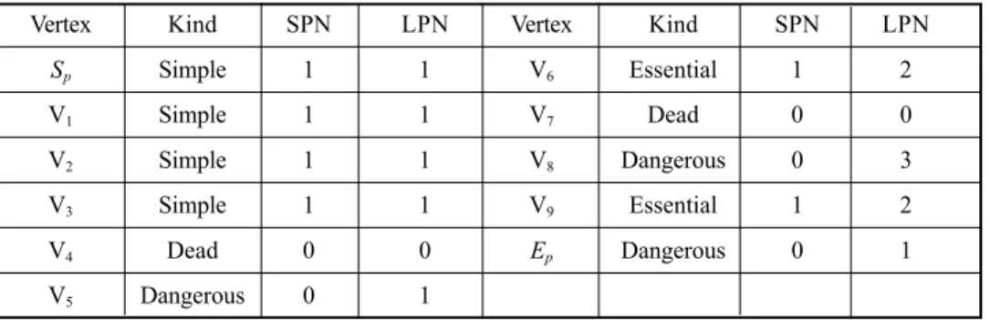
Table 4. The results of analyzing the SPREM graph in Fig. 7.
Vertex Kind SPN LPN Vertex Kind SPN LPN
Sp Simple 1 1 V6 Essential 1 2 V1 Simple 1 1 V7 Dead 0 0 V2 Simple 1 1 V8 Dangerous 0 3 V3 Simple 1 1 V9 Essential 1 2 V4 Dead 0 0 Ep Dangerous 0 1 V5 Dangerous 0 1
Fig. 7. A SPREM graph that is not well-defined.
ity of a complicated system represented by SRPEM, and (3) making a SPREM graph easy to understand and maintain. Algorithm Is-Structured [19] can be used to determine whether a SPREM graph is well-structured.
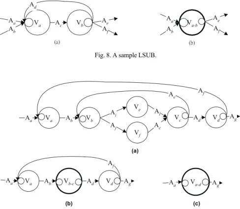
An LSUB can be reduced to an XX vertex whose input and output arcs are those of the entry and exit of the LSUB, respectively, except for the LBA. The inner of an LSUB consists of all the vertices inside the LSUB except for the entry and exit. An LSUB is called a containing LSUB of a vertex V if V is the entry, exit, or an inner of the LSUB. Fig. 8 shows a sample LSUB in (a) and its corresponding XX vertex Va-b, in (b). The LSUB in is
denoted as LSUB(Va, Vb). A nested LSUB can eventually be reduced recursively to an XX
vertex eventually. Fig. 9 shows a sample nested LSUB. LSUB(Vb, Vc) in (a) is reduced to
Vb-c in (b), and LSUB(Va, Vd) in (b) is reduced to Va-d in (c).
Fig. 8. A sample LSUB.
Fig. 9. A sample nested LSUB.
The enaction capability of a well-structured SPREM SP graph can be evaluated by: (1) removing LBAs on each LSUB in SP to make the SP acyclic, (2) evaluating the acyclic SP with Evaluate-Acyclic-SPREM, and (3) adding the LBAs back to SP to refine the evaluation. In a well-structured SP, the entry and exit vertices of an LSUB are X* and *X, respectively, and the LBAs are set to FALSE initially. Thus, the enactability kind of a vertex in LSUB is not changed by the refinement, as mentioned in the earlier discussion about Evaluate-X-Vertex.
7. CONCLUSIONS AND FUTURE WORK
This paper has presented the software project review and evaluation model SPREM. SPREM can be used to express processes with sequence, parallelism, iteration, synchronization, and decision-making behaviors in software projects. Its modeling capa-bility has been demonstrated using an example which describes the spiral model in soft-ware engineering. SPREM is a superset of CPM/PERT and has more concise and natural graphical notation than do (high-level) Petri nets. Several behavioral properties of SPREM have been discussed. For example, its enaction capability can be used to evaluate the pos-sibility that a vertex will enact processes beforehand. Project managers can revise a SPREM graph in order to rescue dead vertices before project execution. Furthermore, enaction ordering allows project managers to calculate the dependency between the processes to be enacted. This might help in computing important information, such as the critical paths among these processes. The detection of MES and DES in a SPREM graph can help project managers avoid pitfalls in modeling. The algorithms Evaluate-Acyclic-SPREM and ate-Cyclic-SPREM, based on several other algorithms, including Evaluate-A-Vertex, Evalu-ate-X-Vertex etc., have been presented to evaluate the enaction capability of acyclic and well-structured SPREMs, respectively.
In addition, some comparisons between SPREM and Petri nets have been discussed in this paper. The high-level Petri nets are better for modeling a system that needs to keep history information, and they can express a complicated predicate in order to enact a transition. However, SPREM is concise and better for modeling a system where the focus is on the current status only. With SPREM, software project managers can get a more natural view from a graph. Some further works need be done in the future:
(1) analysis of the enaction capabilities for a general SPREM graph, (2) detection of the possible execution scenarios of a SPREM graph, and
(3) estimation of the completion time (or cost) for a SPREM graph, including determina-tion of the critical path(s) and the instantiating, running, and terminating times for each process.
REFERENCES
1. P. Armenise, S. Bandinelli, C. Ghezzi, and A. Morzenti, A survey and assessment of software process representation formalisms, International Journal of Software Engi-neering and Knowledge EngiEngi-neering, Vol. 3, No. 3, 1993, pp. 401-426.
2. J. W. Armitage and M. I. Kellner, A conceptual schema for process definitions and models, in Proceedings of 4th International Conference on Software Processes, 1994, pp.153-175.
3. R. Balzar, What we do and dont know about software process, CQS European Ob-servatory on Software Engineering: CASE and Software Quality, October 1990. 4. B. W. Boehm, A spiral model of software development and enhancement, ACM
SIGSOFT Software Engineering Notes, Vol. 11, No. 4, 1986, pp.14-24.
5. S. Bandinelli, A. Fuggetta, and C. Ghezzi, Software process as real time systems: a case study using high-level Petri nets, in Proceedings of International Phoenix Con-ference on Computer and Communication, 1994, pp. 231-242.
6. S. C. Bandinelli and A. Fuggetta, Software process model evolution in the SPADE environment, IEEE Transaction on Software Engineering, Vol. 19, No. 12, 1993, pp. 1128-1144.
7. S. Bandinelli, A. Fuggetta, L. Lavazza, M. Loi, and G. P. Picco, Modeling and improv-ing an industrial software process, IEEE Transaction on Software Engineerimprov-ing, Vol. 21, No. 5, 1995, pp. 440-454.
8. B. Curtis, M. I. Kellner, and J. Over, Process Modeling, Communication of ACM, Vol. 35, No. 9, 1992, pp. 75-90.
9. C. W. Dawson and R. J. Dawson, Clarification of node representation in generalized activity networks for practical project management, International Journal of Project Management, Vol. 12, No.2 1994, pp. 81-88.
10. S. E. Elmaghraby, An algebra for the analysis generalized activity networks, Man-agement Science, Vol. 10, No. 3, 1964, pp. 494-514.
11. W. Emmerich and V. Gruhn, FUNSOFT Nets: A Petri-Net based software process modeling language, in Proceedings of the 6th International Workshop on Software Specification and Design, 1991, pp. 175-184.
12. H. Esiner, A generalized network approach to the planning and scheduling of a re-search project, Operation Rere-search, Vol. 10, No. 1, 1962, pp. 115-125.
13. C. Fernstrom, Process weaver: adding process support to UNIX, in Proceedings of 3rd International Conference on Software Process, 1993, pp. 2-11.
14. A. Fuggetta and C. Ghezzi, State of the art and open issues in process-centered soft-ware engineering environment, Journal of System Softsoft-ware, Vol. 26, No. 1, 1994, pp. 53-60.
15. H. J. Genrich, Predicate/transition nets, in Advances in Petri Nets, 1986, W. Brauer, W. Reisig, and G. Rozenberg, Eds. New York: Springer-Verlag, 1987, pp. 3-43.
16. C. Ghezzi, D. Mandrioli, S. Morasca, and M. Pezze, A unified high-level Petri net formalism for time-critical systems, IEEE Transaction on Software Engineering, Vol. 17, No. 2, 1991, pp. 160-172.
17. K. Jensen, Colored Petri nets and the invariant method, Theoretical Computing Science, Vol. 14, No. 3, 1981, pp. 317-336.
18. B. S. Liang, M. F. Chen, and F. J. Wang, A distributed software process engineering environment, in Proceedings of Workshop of Distributed System Technology and Application, 1997, Taiwan, R.O.C., pp. 531-538.
19. B. S. Liang and F. J. Wang, A software project review and evaluation model, SPREM, Technical Report CSIE-97-1003, Department of Computer Science and Information Engineering, National Chiao-Tung University, March 1997.
20. L. C. Liu and E. Horowitz, A formal model for software project management, IEEE Transaction on Software Engineering, Vol. 15, No. 10, 1989, pp. 1280-1293.
21. J. Magott and K. Skudiarski, Combing generalized stochastic Petri networks for the performance evaluation of concurrent process, in Proceedings of IEEE TH0288-1/89/ 0000/0249, 1989, pp. 249-256.
22. M. A. Marsan, G. Balbo, and G. Gonte, A class of generalized stochastic Petri nets for the performance evaluation of multiprocessor system, ACM Transaction on Com-puter System, Vol. 2, No. 2, 1984, pp. 93-122.
23. I. R. McChesney, Toward a classification scheme for software process modeling approach, Information and Software Technology, Vol. 37, No. 7, 1996, pp. 363-374. 24. P. Merlin and D. J. Faber, Recoverability of communication protocol, IEEE
Transac-tions on Communication, Vol. 24, No. 9, 1976, pp. 1036-1045.
25. C. S. Park, G.S. Lee, and J. M. Yoon, An executable software project management model by beta-distributed stochastic Petri nets, in Proceedings of IEEE TENCON (Region 10 Conference), 1993, pp. 430-434.
26. R. S. Pressman, Software Engineering: A Practitioners Approach, McGRAW-Hill International, 1993, pp. 29.
27. A. A. B. Pritsker and G. E. Whitehouse, GERT: Graphical evaluation and review technique part I: fundamentals, Journal Industry Engineering, Vol. 17, No. 3, 1966, pp. 267-274.
28. C. Ramchandani, A study of asynchronous concurrent systems by timed Petri nets, Technical Report, 120, Project MAC, Massachusetts Institute Technology, February 1974.
29. C. V. Ramamoorthy and G. S. Ho, Performance evaluation of asynchronous concur-rent systems by Petri nets, IEEE Transactions on Software Engineering, Vol. 6, No. 5, 1980, pp. 440-449.
30. R. W. Sebesta, Concepts of Programming Languages, Addison-Wesley, 1996, pp. 309-313.
31. I. Thomas, The strengths and weaknesses of process modeling formalisms, in Pro-ceedings of 7th International Software Process Workshop, 1991, pp. 2-9.
APPENDEX---A
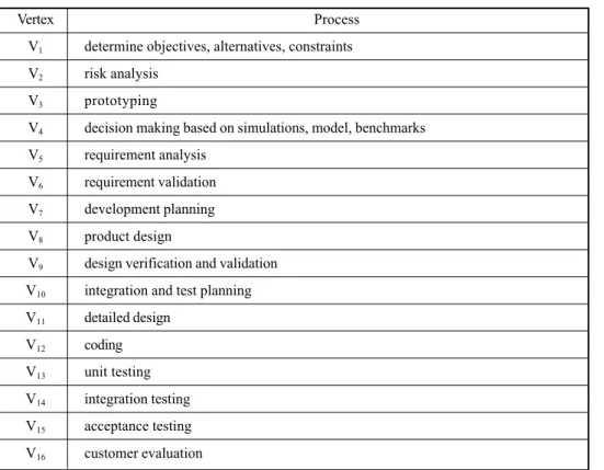
Table 5. The vertex processes in the example shown in Fig. 2.
Vertex Process
V1 determine objectives, alternatives, constraints
V2 risk analysis
V3 prototyping
V4 decision making based on simulations, model, benchmarks
V5 requirement analysis
V6 requirement validation
V7 development planning
V8 product design
V9 design verification and validation
V10 integration and test planning
V11 detailed design V12 coding V13 unit testing V14 integration testing V15 acceptance testing V16 customer evaluation
APPENDIX --- B ::::: ALGORITHMS
B -1
Algorithm Evaluate-A-Vertex (SP, V)
Input: SP = < V, A, Sp, Ep, M0 > (a SPREM grapg), VΠV, is an A* vertex.
Output: V.spn, V.lpn, and V.kind.
/* Given a SPREM graph SP and an A* vertex V in SP, output Vs SPN, LPN, and enactability kind. Let V have m input arcs Aj, j = 1 to m, and let each Aj have a
tail Vj.
Suppose that V.kind is set to dead, that V.spn and V.lpn are set to zero initially, and that Vs predecessors have been evaluated already.*/
begin
Table 6. The vertex arcs in the example shown in Fig. 2.
Arc Artifact = State
A1 software = initialized
A2 software = planned
A3 software = risk-analyzed
A4 software = prototype-created
A5 requirement-specification = initialized or modified
A6 requirement-specification = completed
A7 requirement-specification = validated
A8 software = development-planned
A9 product-design-specification = initialized or modified
A10 product-design-specification = completed
A11 product-design-specification = validated
A12 software = integration & test-planed
A13 detailed-design-specification = initialized or modified
A14 detailed-design-specification = completed A15 module = coded A16 module = tested A17 software = integration-tested A18 software = acceptance-tested A19 software = evaluated A20 software = completed
step 1: MaxEN = min1≤ ≤j mVj.lpn + Vj.is True;/* equation (1)*/
MinEN = min min . . ,
1≤ ≤ + 1
j mV spnj V isTrue j ; /* equation (2) */
VIs Dangerous = FALSE; ArcAllTrue = FALSE; step 2: if Has-Exclv-Vex (V)
then return; /* V.kind = dead; V.SPN = 0; V.LPN = 0*/ step 3: for j = 1 to m do
begin
step 3.1: if (Aj.value = FALSE and Vj.kind = dead)
then return; /* V.kind = dead; V.SPN = 0; V.LPN = 0 */ step 3.2: if not VIsDangerous then
begin
if (Vj.type = *X and Vj.kind π dead) or
(Aj.value = FALSE and Vj.type = *A and Vj.kind = dangerous)
then VIsDangerous = TRUE; end; /* of if */
step 3.3: if Aj.value = FALSE then ArcAllTrue = FALSE;
end; /* of for */ step 4: if ArcAllTrue
then return error; /* this case is not allowed in M0*/
step 5: if VIsDangerous step 5.1: then begin
V.kind = dangerous; V.lpn = MaxEn; end;
step 5.2: else begin */" Vj.satisfy one of the following cases:
(1) Aj is TRUE and Vj is *A,
(2) Aj is TRUE and Vj is *X and dead, or
(3) Aj is FALSE, Vj is *A and simple or essential. */
V.lpn = MaxEN; V.spn = MinEN; if (MaxEN =1)
then V.kind = simple else V.kind = essential; end if;
end; */ of Evaluate-A-Vertex */
B-2
Algorithm Evaluate-X-Vertex (SP, V)
Input: SP = <V, A, Sp, Ep, M0 > (a SPREM), V ΠV, is an A* vertex.
Output: V.spn, V.lpn, and V.kind.
/* Given a SPREM SP and an X* vertex V in SP, output Vs SPN, LPN, and kind. Let V have m input arcs Aj, j = 1 to m, and let each Aj have a tail Vj.
Suppose that V.kind is set to dead, that V.spn and V.lpn are set to zero initially, and that Vs predecessor have been evaluated already.
begin step 1: L1 = max V lpnj k j m . − + , ∑ ≤ ≤ 2 0
1 , where k is the number of Vs TRUE input arcs/*
equation (3) */ L2 = 1≤ ≤∑j mVj.lpn /* equation (3) */ NumOfTrueArc = 0; NumOfDead = 0; NumOfPositveVex = 0; ExistNeuDanVex = FALSE; step 2: for j = 1 to m do begin
step 2.1: if (Aj.value = TRUE)
step 2.2: then begin;
NumOfTrueArc = NumOfTrueArc +1; if (Vj.type = * A or Vj.kind = dead)
then NumOfDead = NumOfDead + 1; end;
step 2.3: else begin /* Aj = FALSE */
if ((Vj.type = * A) and (Vj.kind = simple or Vj.kind = essential))
then NumOfPositveVex = NumOfPositveVex +1; if (not ExistNeuDanVex) then
begin
if (Vj.kind = dangerous) or
((Vj.type = *X) and (Vj.kind = simple or Vj.kind = essential))
then ExistNeuDanVex = TRUE; end;
end; /* of if */ end; /* of for */ step 3: case NumOfTrueArc of
step 3.1: case 1: = 1 /*only one Aj = TRUE */
return error; */ This case is not allowed in M0*/
step 3.2: case 2: ≥ = 2 /*two or more Aj = TRUE */
if (NumOfDead < 2) /* NumOfDead ≥ 2 then V is dead */ then V.kind = dangerous; V.lpn = L1; else V.kind = dead; step 3.3: otherwise: /* NumOfTrueArc = 0, i.e., "Aj = FALSE */
V.lpn = L2;
case NumOfPositveVex of
case 1: = 0; /* no positive predecessor */
if (ExistNeuDanVex = TRUE) /* else "Vj are negative, V is dead */
then V.kind = dangerous;
case 2: = 1; /* only one positive predecessor */ V.spn = Vj.spn; kind = Vj.kind
case 3: = 2; /* exactly two positive predecessors */ /* suppose the two predecessors are Vi and Vj */
V.kind = essential; if Vi.spn = 1 and Vj.spn =1
then V.spn = 2 else V.spn = 1;
otherwise: /* ≥ 3, i.e., three or more positive predecessors */ V.kind = essential; V.spn = 1; end case; end case; step 4: return; end; */ of Evaluate-X-Vertex*/ B-3 Algorithm Evaluate-Acyclic-SPREM (SP) Input: SP = <V, A, Sp, Ep, M0 > (a SPREM).
Output: V.spn, V.lpn, and V.kind. for each V in SP.
/* Given a SPREM SP, for each V in SP, output Vs SPN, LPN, and enactability kind. */
begin
/* initialization */ step 1: clear queue Q;
for each vertex V in V do begin
V.kind = dead; */ suppose V.type is defined in SP */ V.spn = 0;
V.lpn = 0; end;
for each arc A in A do begin
A.beenTraversed = FALSE;
if A.value = TRUE /* suppose A.value is defined in SP */ then A.isTrue =1
else A.isTrue = 0; end;
/* traverse SP from Sp firstly */
step 2: Sp.kind = simple; Sp.lpn = 1; Sp.spn = 1;
set the beenTraversed of all output arcs of Sp to TRUE;
for each successor Vm of Sp whose all input arcs with beenTraversed = TRUE do
En-Queue (Q, Vm);
end;
/* traverse the vertices in topological order */ step 3: while not Empty (Q) do
begin
step 3.1: V = De-Queue(Q); /* evaluate a vertex */ step 3.2: if V.type = A*
then Evaluated-A-Vertex (V)
step 3.3: set the beenTraversed of all output arcs of V to TRUE;
step 3.4: for successor Vm of V whose all input arcs with beenTraversed = TRUE do
En-Queuye(Q, Vm);
end;
end; /* of while */ end; /* of Evaluate-SPREM */
Bin-Shiang Liang ( ) received his B.S. and M.S. degrees in computer science and information engineering from National Chiao Tung University in 1991 and 1993, respectively. He is currently a Ph.D. candidate in computer science and information engi-neering at National Chiao Tung University. His research interests include software measurement, software process modeling, process-centric software engineering environ-ment (PSEE), network-centric computing (NCC), ISO 900 standards certification, and Web-based information systems (WIS).
Jenn-Nan Chen ( ) received his B.S. degree in Applied Mathematics from the Chung Cheng Institute of Technology, Taiwan, R.O.C., in 1972. He received his M.S. degree from the Department of Operation Research, Stanford University, U.S.A., in 1976. He then worked at the Chung Shan Institute of Science and Technology Computer Center as a system engineer for seven years. He attended Northwestern University in the spring of 1983 and received his M.S. and Ph.D. degrees in Computer Science from the Department of Electrical Engineering and Computer Science in 1984 and 1986. He is currently the presi-dent of the SAMAR Techtronics Corporation. His interests include software engineering, software quality assurance, software process modeling, object-oriented techniques, and ISO9000 software methodology development.
Feng-Jian Wang ( ) graduated from National Taiwan University, Taipei, Taiwan, R.O.C., in 1980. He received his M.S. and Ph.D. degrees in E.E.C.S. from Northwestern University, U.S.A., in 1986 and 1988. He is currently a professor in the Department of Computer Science and Information Engineering, National Chiao Tung University. His in-terests include software engineering, compiler, object-oriented techniques, distributed system software, and the internet.