Renewable energy, non-renewable energy and economic growth in Brazil

Renewable energy, non-renewable energy and economic growth

in Brazil

Hsiao-Tien Pao

, Hsin-Chia Fu

Department of Management Science, National Chiao Tung University, Taiwan

b_{College of Engineering, Huaqiao University, Quanzhou, China}

a r t i c l e i n f o

Received 21 June 2011 Received in revised form 25 April 2013

Accepted 7 May 2013 Available online 31 May 2013 Keywords:

Renewable sources

Non-hydroelectric renewable energy Non-renewable energy

Granger causality Brazil

a b s t r a c t

This study employs Brazil’s yearly statistics from 1980 to 2010 to explore the causal relationships between the real GDP and four types of energy consumption: non-hydroelectric renewable energy consumption (NHREC), total renewable energy consumption (TREC), non-renewable energy consumption (NREC), and the total primary energy consumption (TEC). The cointegration test reveals a long-run equilibrium among Brazil’s real GDP, labour, capital, and each of the four types of consumption. The development of the Brazilian economy has close ties with capital formation and labour force. The influence of NHREC/TREC on real output is positive and significant, while the impacts by NREC/TEC are insignificant. The results from the vector error correction models reveal a unidirectional causality from NHREC to economic growth, a bidirectional causality between economic growth and TREC, and a unidirectional causality from economic growth to NREC or TEC without feedback in the long-run. These findings suggest that Brazil is an energy-independent economy and that economic growth is crucial in providing the necessary resources for sustainable development. Expanding renewable energy would not only enhance Brazil’s economic growth and curb the deterioration of the environment but also create an opportunity for a leadership role in the international system and improve Brazil’s competition with more developed countries.

& 2013 Elsevier Ltd. All rights reserved.

Contents

1. Introduction . . . 381

1.1. Brief literature review . . . 382

1.2. Renewable energy in Brazil. . . 382

2. Data analysis . . . 383

3. Model and methodology . . . 384

3.1. Neo-classical production model . . . 384

3.2. Econometric methodology . . . 385

3.3. Constancy of cointegration space . . . 385

4. Empiricalfindings . . . 385

4.1. Results of unit roots and co-integration tests . . . 385

4.2. Results of Granger causality tests . . . 387

5. Conclusion and policy implications . . . 389

Acknowledgement. . . 391

References . . . 391

1. Introduction

According to the 2012 International Energy Outlook by the Energy Information Administration, the worldwide total renew-able energy consumption has been increasing. The growth rate Contents lists available atSciVerse ScienceDirect

journal homepage:www.elsevier.com/locate/rser

Renewable and Sustainable Energy Reviews

1364-0321/$ - see front matter& 2013 Elsevier Ltd. All rights reserved. http://dx.doi.org/10.1016/j.rser.2013.05.004

n_{Corresponding author. Tel./fax:+886 3 5131578.}

was 4.40% in the first decade of the 21st century, including hydropower and non-hydropower growth rates of 3.18% and 12.89%, respectively. During 2011, renewable energy sources supplied an estimated 16.7% of globalfinal energy consumption, and global new investment in renewables increased by 17% due to cost reductions and technological innovations in renewable energy [1]. New renewable (including small hydro, modern biomass, wind, solar, geothermal, and biofuels) technologies are very suitable for local power generation in rural and remote areas, where the transportation costs of crude oil or natural gas are often prohibitively high, as are those of power transmission. Most developing countries have started to identify and implement programs and policies to improve the structure of the ongoing rural renewable energy markets. Thus, rural energy markets increased more and are more attractive to potential investors. The International Energy Agency estimates that annual investment in the rural energy sector needs to increase more thanfivefold to achieve the wide use of new renewables energy by 2030. All of these factors point to a brighter future for renewable energy.

1.1. Brief literature review

Empirical studies of the relationship between energy consump-tion and economic growth have been conducted intensively for different economic regions or countries over the past two decades (e.g.,[2–14]). Most of the literature has focused on the relationship between electricity consumption and income, or the nexus of energy-income-emissions. These nexus suggest that economic growth is closely related to energy consumption because eco-nomic or industrial activities require energy consumption. On the other hand, more efficient energy development or use requires the financial support of a strong economy. Therefore, the directions of causality between different types of energy consumption and economic growth merit examination.

In the early 21st century, the relationship between renewable energy consumption and economic growth has attracted signi fi-cant research interest. The commonly employed methodologies include the forecast error variance decomposition analysis model, the bivariate error correction model, the Toda–Yamamoto proce-dure within a framework of production function, and the multi-variate error correction model within a framework of production function. Using a generalised forecast error variance decomposi-tion analysis, Sari and Soytas [15] found that different energy consumption items have different effects on real output and energy consumption appears to be almost as important as employ-ment with respect to economic developemploy-ment in Turkey, where lignite, waste, oil and hydraulic power comprise the top four among all alternative sources of energy. For the US, Ewing et al.

[16] found out that unexpected shocks to coal, natural gas and fossil fuel energy sources have the greatest impacts on the variation of real output, while renewable energy consumption of several types also exhibit considerable explanatory power. Never-theless, consumption of none of the energy sources above can explain the forecast error variance of industrial output better than employment. Using a bivariate panel error correction model, Sadorsky [17] presented evidence of bidirectional causality between non-hydroelectric renewable energy consumption and economic growth in emerging economies. Using the Toda –Yama-moto procedure within the framework of a production model for analysing data of the US, Payne[18]found no evidence of a causal relationship between total renewable or non-renewable energy consumption and real output, although Payne [19] and Yildirim et al. [20] found unidirectional causality from biomass energy consumption to real output. Using a multivariate panel error correction model within a framework of production model, Apergis and Payne [21] found evidence of bidirectional short-and long-run causality between non-hydroelectric renewable

energy consumption and economic growth for OECD countries. Apergis and Payne[22, 23] discovered evidence of bidirectional short- and long-run causality between total renewable energy consumption and economic growth for Eurasia and Central America countries, respectively. However, no publications explore the causal relationships between renewable/non-renewable energy consump-tion and economic growth in sustainable countries such as Brazil. In the past two decades, Brazil has achieved a development model that combines social inclusion with sustained economic growth and the balanced use of natural resources[24]. Moreover, over the next 10 years, the projected annual GDP growth rate will reach approxi-mately 5.1% [25]. Therefore, this study attempts to analyse the above relationships in Brazil.

1.2. Renewable energy in Brazil

Brazil currently hosts one of the cleanest energy matrices of the industrialised world, with 44.1% of energy coming from renewable sources, and approximately 89% of all electricity supply coming from renewable energy sources, with 81.7% of all electricity supply coming from hydropower. However, non-hydro renewable elec-tricity has a very high compound annual growth rate of 10.01%. Brazil_{’s renewable power capacity is the world’s third largest after} China and the United States. Its hydropower capacity is the world’s second largest after China, and continues to increase rapidly[1].

Two leading and far-reaching programs, The Alternative Energy Sources Incentive Program (PROINF) and The Ten Year Energy Expansion Plan (PDE), have been proposed by the Brazilian government to enhance Brazil’s manufacturing sector and to create a scenario of sustainable energy supply in technical, envi-ronmental, and economic aspects. The PROINF, developed in 2002, attempts to increase the production of electric energy using renewable sources such as biomass, small hydro, and wind plants. PROINFA aims to increase the share of new renewables (biomass, wind, and small hydro) to 10% of the electricity consumption of Brazil in 2020[25]. The Ten Year Energy Expansion Plan aims to ensure the balanced expansion of energy supply and to assist in creating a solid foundation for economic growth in the country

[26]. In addition, there are a large number of renewable energy projects in progress, such as constructing many new wind farms, launching the‘My Home, My Life’ programme using solar energy for all new houses, constructing small hydroelectric plants to meet the energy demands of small urban centres and rural areas, and executing waste management projects to help poor families become suppliers of biomass power plants by using waste from acai to enhance the manufacturing sector and to help the country’s economy. Furthermore, to cope with the Brazilian renewable energy policies and plans, many governmental or private new renewable energy manufacturers, e.g., Soletrol Inc. for solar energy, Vestas and Gamesa Inc. for wind turbine, Sade Vegesa Inc. for small hydro turbine, and the Brazilian Association of Industry Biomass and Renewable Energy Council, have been established to meet the demands of the new renewable energy trend.

For hydropower in Brazil, construction of two huge hydro-electric dams, Santo Antonio and Jirau, began in 2008 on the Madeira in Brazil. While respecting the environment, the planning of new dams can provide approximately 11% of the country’s electricity. These projects create employment opportunities and promote substantial investments of the consortium into dam construction. Moreover, Brazil has a large number of small hydro-electric plants to meet the energy demands of small urban centres and rural areas. This heavy reliance on hydroelectric power illustrates the risk inherent in unreliable water sources. In the early 2000s, a drought in Brazil prompted severe energy shortages and hurt the country_{’s economy which highlighted the urgent} need to diversify its energy portfolio. Recently, the main components

of Brazil’s energy structure have been biomass, wind, solar, and nuclear.

Brazil’s capacity for generating biomass power is the world’s second largest after the United States and accounted for 24.9% of world’s total ethanol fuel production in 2011[1]. Its production of ethanol and biodiesel are the world’s second largest and fourth largest, respectively, and both have been growing steadily. After the oil shocks of the 1970s, the Brazilian government has con-sistently promoted sugarcane ethanol as an alternative source of energy. In 2011, sugarcane products accounted for 15.7% of Brazil_’s domestic supply. Brazil’s Braskem SA, the largest petrochemical company in Latin America, produces polyethylene and polypropy-lene from 100% sugarcane-derived ethanol. This green ethypolypropy-lene plant is an important indicator that Brazil may become a global leader in sustainable chemicals. Recently, Brazilian sugarcane ethanol was designated as an advanced biofuel with 61% lower lifecycle greenhouse gas emissions than petroleum fuels. Brazil is considered to be the world’s first sustainable biofuel economy, a leader in the biofuel industry, and a policy model for other countries. Its sugarcane ethanol has been the most successful alternative fuel to date[27]. Moreover, Brazil administers a waste management project to help poor families become suppliers of biomass power plants by using waste from acai. This innovative recycling approach will turn a growing environmental problem into a green business opportunity, create new jobs, and provide leadership to the rest of the world in generating ef_{ficient and} sustainable clean energy[1].

Brazil has strong winds throughout the year, especially in the low rainfall dry season, which makes wind power a potential supplement to Brazil’s water power. In 2009, 10 projects for wind farms were under construction, and in 2010, 45 projects began construction in several States. These projectsfinanced by PROINFA account for over 95% of wind energy installations [25]. Brazil’s wind power capacity has increased by a massive 24.2% from 2011 and is almost half of the total Latin American. The price of wind power has dropped to less than electricity from natural gas. The Brazilian Wind Energy Association has reported a goal of achieving 10 GW of wind energy capacity by 2020, increasing from the current 605 MW, and having another 450 MW under construction

[27]. Developing wind power sources can enhance energy security, reduce emissions, and create jobs for Brazil. The Ten Year Plan indicates that hydroelectric or wind projects are to be carried out in subsequent years to meet the anticipated demand[26]. Globally, wind power has seen the highest expansion rate among all renewable energy alternatives in the world. With an average annual growth rate of 27% since 1990, it accounted for almost 40% of new renewable capacity in 2011.

Solar thermal heating technologies also contribute significantly to hot water production in Brazil. Measured by the solar heating market of 2010, the newly installed capacity in Brazil is the world’s sixth largest, the country’s total installation is the world’s fifth largest, and the_{five-year compound annual growth rate is almost} 18%. The rapidly expanding market is driven by household applica-tions (57%), industry, commerce, and services sectors (23%), and the ‘My Home, My Life’ social housing programme (20%), a seven project

that began in 2007 uses solar energy for all new houses[1]. In short, Brazil approaches the use of solar energy in two ways, the thermal route used mainly for heating and power generating, and photo-voltaic panels for lighting, pumping, and communication[25].

Furthermore, nuclear power provides approximately 3% of Brazil’s electricity from two nuclear reactors (Angra 1 and 2). The plant for Angra 3 was scheduled to begin operation in 2009 and is expected in operation at 2016. The Brazilian government has proposed building two new nuclear plants after 2020 to meet the needs of the country_{’s fast-growing economy} [28,29]. Economic planners predict that Brazil could become the world’s fifth largest economy in a few years, and the annual GDP growth rate is projected to reach 5.1% over the next 10 years.

The aim of this paper is to explore the causal relationship between real GDP and non-hydro renewable, total renewable, non-renewable, and total primary energy consumption in Brazil. We used a framework based on the neo-classical one-sector aggregate production methodology, where capital, labour and energy are treated as separate inputs. Within this framework, a vector error-correction model (VECM) was employed to test for multivariate cointegration and Granger causality.

Section 2presents the relevant energy and economic data used,

Section 3 outlines the analytical model and econometric metho-dology, and Section 4 provides the empirical findings of the research and the last section concludes the study.

2. Data analysis

Annual data for Brazil’s real GDP, real gross fixed capital formation (GCF), and labour force (LF) from 1980 to 2010 were obtained from the World Development Indicators (WDI). Data for different types of energy consumption, including non-hydro renewable (NHREC), total renewable (TREC; sum of NHREC and hydroelectric (HREC)), and total primary energy consumption (TEC; sum of petroleum, coal, nature gas, hydropower, nuclear, renewable, etc.) were extracted from the Energy Information Administration (EIA). Note that the net consumption does not include energy consumption by the generating units [17]. The value of total non-renewable energy consumption (NREC) is equal to the TEC minus the TREC. Wind and biomass accounted for almost all non-hydro renewable electricity in Brazil, while solar and geothermal accounted for very little. The renewable energy consumption is defined in billions of kilowatt hours. Non-renewable and total primary energy consumptions are measured in quadrillion BTU. Both real GDP and the real grossfixed capital formation are measured in US dollars at 2000 prices. Total labour force is measured in millions.

During the period 1980–2010, TREC and NREC accounted for 37.68% and 62.32% of the TEC with compound annual growth rates of 3.87% and 3.30%, respectively. For renewable power consump-tion, NHREC and HREC accounted for 3.28% and 96.72% of the TREC with compound annual growth rates of 10.01% and 3.85%, respec-tively. Nuclear and wind power accounted for only 0.76% and 0.06% of the TEC, but they had very high compound annual growth

Table 1

Summary statistics for variables, 1980–2010. (Constant 2000 US$ Billion)

(Million) (Billion kt) (Quadrillion Btu)

GDP GCF LF NHREC TREC NREC TEC

Mean 597.41 (143.62) 104.91 (23.70) 74.10 (17.38) 8.54 (7.34) 260.43 (84.73) 4.39 (1.47) 7.04 (2.25)

CV (%) 24.04 22.59 23.46 85.95 32.54 33.49 31.96

rates of 19.39% and 64.79%, respectively. For data analysis and modelling, we considered the disaggregated levels of NHREC, TREC, and NREC and the aggregated level of TREC, due to their high growth rate or high proportion of total energy consumption. The consumption of solar, wind, and nuclear energy is excluded from the modelling analysis, because there was no sufficient reference data during 1980–2010 and because they represent less than 1% of the total energy consumption. Biomass and hydro are also excluded, because biomass and hydro accounted for a high percentage (97.94% and 96.72%) of NHREC and TREC, respectively, and NHREC and TREC are included in the modelling analysis in

Section 3.Table 1displays the summary statistics associated with the seven variables including GDP, GCF, LF, NHREC, TREC, NREC, and TEC. As we can see that the NHREC demonstrated the largest coefficient of variation (85.95%) because of its high growth rate.

Figs. 1and2show the time series of Brazilian data, all of which have demonstrated growth trend over time.

For modelling purposes, all of the above time series data are converted with natural logarithms. The converted time series can be interpreted in growth terms after taking thefirst difference into account.

3. Model and methodology

To investigate the relationship between energy consumption and economic growth, this study used the framework proposed in Apergis and Payne[21–23], which is based on the conventional

neo-classical one-sector aggregate production technology where capital, labour, and energy are treated as separate inputs. That is

Yt¼ f ðKt; Lt; EtÞ ð1Þ

where Y is the aggregate output or real GDP, K is the capital stock, L is the labour, E is the energy-related variable, and subscript t is the time. The inclusion of measures for capital and labour is a means to circumvent the possibility of omitted variable bias[30]. The production function in Eq. (1) can be used to describe the long-run equilibrium relationship between real output and capital, labour, and energy inputs. For the short-run dynamics in factor-output behaviour, the analysis above would also suggest that past changes in capital, labour, and energy could contain useful information for predicting the future changes of output. These implications can be examined using tests for multivariate coin-tegration and Granger causality.

3.1. Neo-classical production model

To assess the different results obtained from considering renewable and non-renewable energy consumptions, the follow-ing production model, includfollow-ing energy-related variables as a proxy for technological progress, is considered[21]:

LGDPt¼ β0þ β1LGCFtþ β2LLFtþ β3LECitþ ut; i ¼ 1; 2; 3; 4 ð2Þ

where LGDP, LGCF, LLF, t, and LECi_{(i¼1, 2, 3) represent natural}

logarithms of real GDP, capital formation, labour force, determi-nistic time trend, respectively, and three different types of energy 300 400 500 600 700 800 900 1,000 80 82 84 86 88 90 92 94 96 98 00 02 04 06 08 10 GDP (Billion) 60 80 100 120 140 160 180 80 82 84 86 88 90 92 94 96 98 00 02 04 06 08 10 GCF (Billion) 40 50 60 70 80 90 100 110 80 82 84 86 88 90 92 94 96 98 00 02 04 06 08 10 LF (Million)

Fig. 1. Time series plots of real GDP, real grossfixed capital formation, and labour force, 1980–2010.

0 5 10 15 20 25 30 35 80 82 84 86 88 90 92 94 96 98 00 02 04 06 08 10 NHREC (Billion KilowattHours)

120 160 200 240 280 320 360 400 440 80 82 84 86 88 90 92 94 96 98 00 02 04 06 08 10 TREC (Billion KilowattHours)

2 3 4 5 6 7 8 80 82 84 86 88 90 92 94 96 98 00 02 04 06 08 10 NREC (Quadrillion Btu)

3 4 5 6 7 8 9 10 11 12 80 82 84 86 88 90 92 94 96 98 00 02 04 06 08 10 TEC (Quadrillion Btu)

consumption (including non-hydroelectric (LNHREC), total renew-able (LTREC), and non-renewrenew-able (LNREC). GCF is considered as a proxy for the capital stock variable. For aggregated level, the LEC variable in Eq. (2) is replaced by LTEC. The error term, ut, is

assumed to be independent and identically distributed with a zero mean and a constant variance. Variables in natural logarithms can be interpreted in growth rate after taking thefirst difference into account. The coefficients βj; j¼1, 2, 3 can be interpreted as

elasticity estimates.

3.2. Econometric methodology

The empirical analysis tests for the existence of a long-term relationship among the variables (estimation of Eq.(2)), while the vector error-correction model captures the short-run dynamics of the variables. The analysis is performed in three steps, thefirst of which is to verify the order of the integration of the variables, because various cointegration tests are only valid if the variables have the same order of integration. Three different unit root tests, namely Augmented Dickey–Fuller (ADF)[31], the Phillips–Perron (PP)[32]and Kwiatkowski–Phillips–Schmidt–Shin (KPSS)[33]are used to investigate the stationarity and the order of the integration of the variables. In terms of literature, tests designed on the basis of the null hypothesis that a series is I(1) have a low power of rejecting the null. Hence, KPSS is sometimes used to complement the widely used ADF and PP tests to obtain robust results.

In the second step, when all of the series are found to be integrated of the same order, the Johansen maximum likelihood method[34]is used to test the cointegration relationship between the variables in Eq. (2). The model selection is guided by the Akaike Information Criterion (AIC) and Schwarz Bayesian Criterion (SBC). The existence of cointegration indicates that there are long-run equilibrium relationships among the variables, and thereby, Granger causality exists among them in at least one direction

[35,36].

In the last step, if all of the variables are I(1) and cointegrated, the error correction model (ECM) is used to correct any disequili-brium in the cointegration relationship, that may have been captured by the error correction term (ECT), and to test for long-run and short-long-run causalities among the cointegrated variables. The ECM for Eq.(2)is specified as follows:

ΔLGDPt¼ γ10þ ∑ m1 i¼ 1γ11iΔLGDPt−iþ ∑ n1 i¼ 1γ12iΔLGCFt−i þ ∑p1 i¼ 1γ13iΔLLFt−iþ ∑ q1

i¼ 1γ14iΔLECt−iþ δ1

ECTt−1þ μ1t ð3aÞ ΔLGCFt¼ γ20þ ∑ m4 i¼ 1γ21iΔLGDPt−iþ ∑ n4 i¼ 1γ22iΔLGCFt−i þ ∑p4 i¼ 1γ23iΔLLFt−iþ ∑ q4

i¼ 1γ24iΔLECt−iþ δ2

ECTt−1þ μ2t ð3bÞ ΔLLFt¼ γ30þ ∑ m3 i¼ 1γ31iΔLGDPt−iþ ∑ n3 i¼ 1γ32iΔLGCFt−i þ ∑p3 i¼ 1γ33iΔLLFt−iþ ∑ q3

i¼ 1γ34iΔLECt−iþ δ3

ECTt−1þ μ3t ð3cÞ ΔLECt¼ γ40þ ∑ m2 i¼ 1γ41iΔLGDPt−iþ ∑ n2 i¼ 1γ22iΔLGCFt−i þ ∑p2 i¼ 1γ43iΔLLFt−iþ ∑ q2

i¼ 1γ44iΔLECt−iþ δ4

ECTt−1þ μ4t ð3dÞ

where

ECTt−1¼ LGDPt−1−a0−a1LGCFt−1−a2LLFt−1−a3LECt−1 ð3eÞ

is derived from the long-term cointegration relationship obtained from Eq. (2). The sign Δ is the first-difference operator; the optimum lag lengths mi, ni, piand qiare determined on the basis

of Akaike’s information criteria; and mitare the serially

uncorre-lated error terms. In the ECM model, the LEC variable inEq. (3)is replaced by LNHREC, LTREC, LNREC, and LTEC, sequentially, to investigate the causal relationships between non-hydro renew-able, total renewrenew-able, non-renewrenew-able, and total energy consump-tion and economic growth. The parameter δ1 is the adjustment

coef_{ficient which measures the speed at which the values of LGDP} came back to long-term equilibrium levels, once LGDP violates the long-run equilibrium relationship.

The ECM represented byEq. (3)includes both the dependent variables with their own lags and the previous disequilibrium in terms of ECTt−1. This specification can test the short-run and

long-run causalities among cointegrated variables. In terms of short-long-run causality in Eq. (3a) and (3d), the causality runs from energy consumption to economic growth if the joint null hypothesis, γ14i¼0, ∀i is rejected via a Wald test, whereas the causality runs

from economic growth to energy consumption if the joint null hypothesis γ41i¼0, ∀i is rejected. With respect to long-run

caus-ality, if the null hypothesisδ1¼0 is rejected, economic growth will

react to deviation from the long-run equilibrium. If the null hypothesis δ4¼0 is rejected, then the energy consumption will

react to the deviation from the long-run equilibrium. 3.3. Constancy of cointegration space

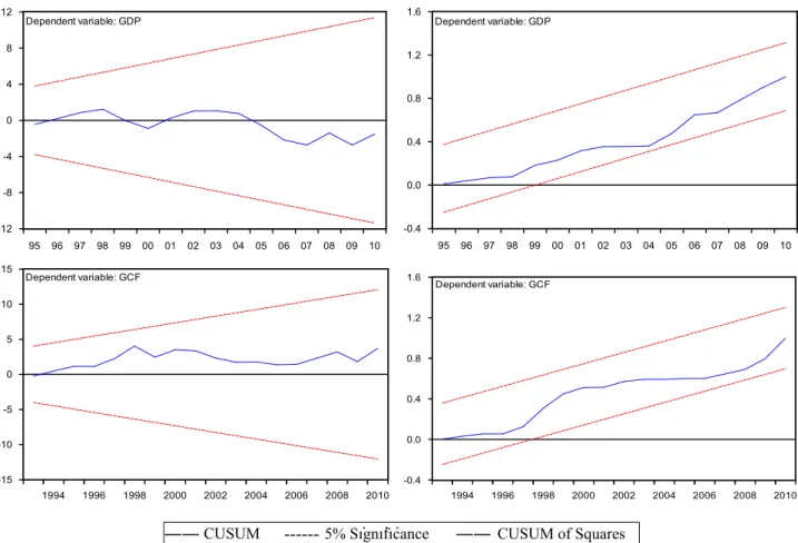
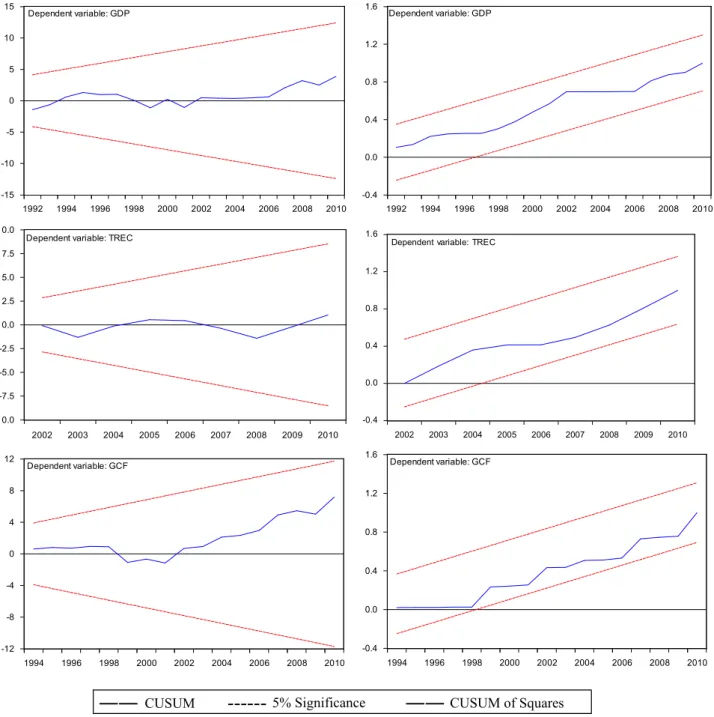
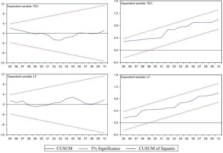
An important issue with ECM is that the parameter estimates may change over time, and the unstable parameters may lead to misspecification. If any structure break exists, the ECM parameters and variables should be adjusted to reflect the structure break[13]. We employ the Brown et al. [37] tests popularly known as the cumulative sum (CUSUM) and cumulative sum of squares (CUSUMSQ) tests to check for the stability of parameters and regressions in the ECM. Based on the recursive regression resi-duals, the CUSUM and CUSUMSQ statistics are updated recursively and plotted against the model’s break points. Thus, the coefficients of a given regression are stable if the plots of the statistics fall within critical bounds of 5% significance. Once the ECM is estimated, we perform CUSUM and CUSUMSQ stability tests on ECM equations. This exercise is only for the equation that contains significant ECT, because the coefficient of ECT represents the long-term relationship[9].

4. Empiricalfindings

The annual data for Brazil’s real GDP, capital, labour and different types of energy consumptions in the period between 1980 and 2010 was used to estimate the production models of Eq. (2), and to test for the multivariate cointegration and the Granger causality ofEq. (3).

4.1. Results of unit roots and co-integration tests

The time series properties of the variables in Eq. (2) are evaluated through three different unit root tests, namely ADF, PP, and KPSS. Each of the seven time series appears to contain a unit root in their levels but are stationary in their first difference, indicating that they are integrated at order one, i.e., I(1). The results are displayed inTable 2.

The next step is to test whether the variables in Eq. (2) are cointegrated. The results for the Johansen test using no lags and intercepts in the model are shown in Table 3. The trace and eigenvalue tests reject the hypothesis of no cointegrating equation

at a 5% level of significance for Eq.(2). The results in panels A–D of

Table 3indicate the existence of at least one cointegrating vector for (LGDP, LGCF, LLF, LECi) combinations at the 5% significance level, where LECi_{; i¼1,…,4 are LNHREC, LTREC, LNREC, and LTEC,}

respectively. The resulting parameter estimates for Eq. (2) are reported inTable 4. The model properties are evaluated using two diagnostic tests, the Jarque and Bera (JB) test[38]for normality and the Ramsey RESET test[39]for functional form misspeci fica-tion. The test results reported inTable 4show that all models pass the diagnostic tests, indicating no significant deviations from the desired model properties. Thus, Eq.(2)is suitable for each type of energy consumption. That is, real GDP, capital formation, labour force, and each of the four type’s energy consumption share a common trend in the long run.

As far as the results of four cointegration vectors normalised on GDP are concerned, the coefficients of LGCF and LLF are found to affect the level of development significantly and positively by approximately 0.37% and 0.60% on average, respectively. This suggests that the process of economic development is heavily dependent on investment and labour in Brazil. The coefficients of NHREC and TREC are positive and significant, while the coeffi-cients of NREC and TEC are far from significant. A 1% increase in non-hydro renewable energy consumption increases real GDP by 0.06%, and a 1% increase in total renewable energy consumption increases real GDP by 0.20%. This suggests that renewable energy consumption is more sensitive to real output, while the impact of non-renewable or total primary energy consumption on real output is very small. Our findings highlight the importance of Table 3

Results of Johansen’s cointegration test.

Panel A: LGDP, LNHREC, LGCF, and LLF variables; no lags

Eigenvalue Trace stat. 5% critical value Max Eigen. stat. 5% critical value Number of co-integrations

0.92 114.67nnn _{54.08 76.28}nnn _{28.59 None}

0.50 38.40nn 35.19 20.76nn 22.30 At most 1

0.30 17.64 20.26 10.52 15.89 At most 2

Panel B: LGDP, LTREC, LGCF, and LLF variables; no lags

0.90 99.05nnn _{54.08 69.93}nnn _{28.59 None}

0.50 29.12 35.19 20.77 22.30 At most 1

Panel C: LGDP, LNREC, LGCF, and LLF variables; no lags

0.90 105.91nnn _{54.08 68.82}nnn _{28.59 None}

0.55 37.09nn 35.19 24.17nn 22.30 At most 1

0.27 12.92 20.26 9.41 15.89 At most 2

Panel D: LGDP, LTEC, LGCF, and LLF variables; no lags

0.90 100.51nnn _{54.08 69.19}nnn _{28.59 None}

0.45 31.32 35.19 17.89 22.30 At most 1

Note: The optimal lag lengths are selected using AIC. nnDenote significance on the 5% level.

nnn_{Denote significance on the 1% level.}

Table 4

Coefficients of Eq.(2)for different types of energy consumption, 1980–2010.

LGCF LLF LNHREC LTREC LNREC LTEC Intercept R2 _{JB RESET}

0.343*** 0.554*** 0.057** _{2.301*** 0.9910 0.76 1.02} (9.02) (7.94) (2.13) (6.50) [0.68] [0.32] 0.365*** 0.434*** 0.201** 1.710*** 0.9912 1.49 0.73 (12.24) (3.96) (2.42) (16.24) [0.48] [0.40] 0.409*** 0.731*** −0.035 1.397*** 0.9897 1.55 1.25 (11.52) (12.48) (−0.72) (5.22) [0.46] [0.28] 0.395*** 0.694*** −0.001 1.571*** 0.9895 1.33 1.75 (10.77) (6.92) (−0.02) (4.21) [0.51] [0.20]

Note: Figures in parenthesis indicate t statistics. p-Values are reported in brackets. nnDenote significance on the 5% level.

nnn_{Denote significance on the 1% level.}

Table 2

Results of unit roots tests, 1980–2010.

Variable ADF PP KPSS

Level 1st diff. Level 1st diff. Level 1st diff.

LGDP 1.19 −3.79a 1.79 −4.73a 2.46a 0.24 LGCF −0.19 −4.92a _{−0.06 −5.07}a _2.29a _0.21 LLF −0.65 −4.75a _{−0.73 −4.75}a _0.25a _0.05 LNHREC 1.53 −4.77a −1.75 −4.77a 2.08a 0.34 LTREC −1.01 −5.64a −1.04 −5.63a 1.80a 0.13 LNREC −0.53 −7.79a _{−0.26 −7.94}a 0.80a 0.09 LTEC −0.68 −7.25a _{−0.26 −7.42}a 2.42a 0.06 Note: The nulls of all tests except for the KPSS are unit roots. The null of KPSS states that the variable is stationary. Individual intercepts are included in test regressions.

a

renewable energy sources within the Brazilian energy portfolio. Brazil’s elasticity of real GDP to renewable energy consumption is greater than that found by Apergis and Payne[22]for Eurasia, and lower than those found by Apergis and Payne [23] for Central American countries as a whole.

4.2. Results of Granger causality tests

Cointegration implies the existence of causality, at least in one direction. However, it does not indicate the direction of the causal relationship. Hence, to shed light on the direction of causality,

Table 7

Results of causality tests for non-renewable energy consumption model. Source of causation (independent variables)

Short-run Chi-square-statistics Long-run t statistics

ΔLGDP ΔLNREC ΔLGCF ΔLLF ECT

ΔLGDP 2.81 7.90nn 12.62nnn 1.40 (0.17)

ΔLNREC 1.58 13.02nnn _35.94nnn _−8.23nnn_(−0.54)

ΔLGCF 12.86nnn _{3.44 1.44 −3.04}nnn_(−0.56)

ΔLLF 23.84nnn _21.29nnn _28.66nnn _4.25nnn_(0.11)

Note: The optimal lag lengths are selected using AIC. Figures in parentheses are coefficients. nn_{Indicate 5% level of significance.} nnn_{Indicate 1% level of significance.}

Table 8

Results of causality tests for total primary energy consumption model. Source of causation (independent variables)

Short-run Chi-square-statistics Long-run t statistics

ΔLGDP ΔLTEC ΔLGCF ΔLLF ECT

ΔLGDP 0.23 10.02nnn 1.67 −1.18 (−0.08)

ΔLTEC 18.03nnn 7.64nn 35.58nnn −5.24nnn_(−0.86)

ΔLGCF 5.51n _{0.37 4.00 −1.32 (−0.44)}

ΔLLF 38.41nnn _35.15nnn _42.06nnn _7.99nnn_(0.21)

Note: The optimal lag lengths are selected using AIC. Figures in parentheses are coefficients. n_{Indicate 10% level of significance.} nn_{Indicate 5% level of significance.}

nnn_{Indicate 1% level of significance.}

Table 6

Results of causality tests for total renewable energy consumption model. Source of causation (independent variables)

Short-run Chi-square-statistics Long-run t statistics

ΔLGDP ΔLTREC ΔLGCF ΔLLF ECT

ΔLGDP 1.70 8.51nn _{1.69 −2.41}nn_(−0.16)

ΔLTREC 3.16 12.03nnn _7.39nn _−6.07nnn_(−0.04)

ΔLGCF 12.40nnn _3.37n _15.82nnn _−3.36nnn_(−0.67)

ΔLLF 12.05nnn _{1.07 11.81}nnn _{−0.43 (−0.02)}

Note: The optimal lag lengths are selected using AIC. Figures in parentheses are coefficients. n_{Indicate 10% level of significance.} nn_{Indicate 5% level of significance.}

nnn_{Indicate 1% level of significance.}

Table 5

Results of causality tests for non-hydroelectric renewable energy consumption model. Source of causation (independent variables)

Short-run Chi-square-statistics Long-run t statistics

ΔLGDP ΔLNHREC ΔLGCF ΔLLF ECT

ΔLGDP 42.83nnn _58.59nnn _9.44nn _−11.40nnn_(−0.55)

ΔLNHREC 23.01nnn _21.44nnn _14.47nnn _{−0.75 (−0.12)}

ΔLGCF 0.14 2.88 3.67 −3.48nnn_(−0.97)

ΔLLF 9.20nn _{1.83 15.49}nnn _{0.60 (0.03)}

Note: The optimal lag lengths are selected using AIC. Figures in parentheses are coefficients. nn_{Indicate 5% level of significance.} nnn_{Indicate 1% level of significance.}

ECM-based causality tests are performed. Tables 5–8 report the causality results from estimating the vector error correction model for LGDP, LGCF, LLF, and four different types of energy consump-tion. Both the short-run Chi-square statistics and the long-run t statistics are shown for each ECM. The results reported inTable 5

indicate a bidirectional causality between NHREC and economic growth, and unidirectional causality from capital formation and labour force to NHREC in the short run. As for the long-run, there is unidirectional causality from NHREC to economic growth and bidirectional causality between economic growth and capital formation. Indeed, the short- and long-run Granger causality between economic growth and NHREC is partially similar to the previous research by Sadorsky[17]for 18 emerging countries as a whole and Apergis and Payne’s[21]results for OECD countries as a whole. The results of Table 6 indicate unidirectional short-run causalities from capital formation and labour force to TREC, and bidirectional causality between capital formation and TREC in the long-run. There also exists bidirectional causality between eco-nomic growth and TREC in the long-run, but no short-run causal relationship between them. This result is partially similar to those reported by Apergis and Payne [22,23] for Eurasia or Central American countries as a whole. As a result, the different causality relationship between NHREC-output and TREC-output is due to the NHREC that only accounts for 3.28% of the TREC during 1980– 2010. The overallfindings of bidirectional causality between NHREC and economic growth in the short-run, unidirectional causality from NHREC to economic growth and bidirectional causality between economic growth and TREC in the long-run highlight the importance of renewable energy sources within the energy port-folio of Brazil. Likewise, economic growth is crucial in providing the necessary resources for the sustainable development.

Table 7reports the causality results obtained from considering NREC. FromTable 7, the short-run dynamics suggest unidirectional causality from capital formation to NREC and bidirectional caus-ality between NREC and labour force. The ECT is statistically significant at the 1% level in capital formation, labour force, and NREC equations. This suggests that there is bidirectional causality between both NREC and capital formation and between NREC and labour force, and unidirectional causality from economic growth to NREC without feedback in the long-run. Comparing the results of

Tables 7and8show that there is bidirectional causality between economic growth and total renewable energy consumption, but no causality running from non-renewable energy consumption to economic growth. As for the long-run, the magnitudes of the adjustment coefficients are −0.16 for the real GDP equation in

Table 6. Thus, near-complete adjustments to the long-run equili-brium induced by changes in real GDP would take approximately 6 years after a shock occurs.

At the aggregate level, the causality results for TEC shown in

Table 8suggest that unidirectional short-run causality from capital formation and economic growth to TEC and bidirectional causality between TEC and labour force. The ECT is statistically significant at the 1% level in both the labour force and TEC equations. This suggests that there is bidirectional causality between TEC and labour force, and unidirectional causality from economic growth and capital formation to TEC in the long-run. The bidirectional short- or long-run causality between NREC/TEC and labour force and the lack of either short- or long-run causality running from NREC/TEC to economic growth suggest that Brazil is an energy-independent economy. Indeed, after the world’s second oil-price shock, the Brazilian government has undertaken an ambitious programme to reduce its dependence on imported oil. At the

beginning of the 21st century, Brazil switched from being a large oil importer to almost being oil independent. Thus, Brazil’s economy is no longer dependent on foreign oil supply.

In testing for parameter constancy in each ECM model, we employed the CUSUM and CUSUMSQ tests to the estimated equations for which there were significant ECT. For the ECM with NHREC variable, the ECTs in the GDP and GCF equations are significant. The CUSUM and CUSUMSQ plots for each equation are shown inFig. 3. For the ECM with TREC variable, the ECTs in the GDP, TREC, and GCF equations are signi_{ficant. For the ECM with} NREC variable, the ECTs in the NREC, GCF, and LF equations are significant. For the ECM with TEC variable, the ECTs in the TEC and LF equations are significant.Figs. 4,5, and6show the CUSUM and CUSUMSQ plots of these equations. As seen, neither the CUSUM nor the CUSUMSQ test statistics exceeds the bounds of the 5% level of significance, indicating an overall constancy in the regression equations.

5. Conclusion and policy implications

This study analyses the long-run dynamic relationship between Brazil’s renewable and non-renewable energy consumption and its economic growth, treating non-hydro renewable energy consump-tion separately because of its very high 30-year compound annual growth rate of 10.01%. The data used were published by the Brazilian government during the period between 1980 and 2010. The conventional neo-classical one-sector aggregate production technology treatment was employed, where capital, labour, and energy are treated as separate inputs. The results reveal common trends in the long-run between real output, capital formation, labour force, and each of the four type’s energy consumption including NHREC, TREC, NREC, and TEC. Brazil’s economic devel-opment is heavily dependent on investment as well as labour. Furthermore, real output is quite sensitive to renewable energy consumption, while the impact of non-renewable or total primary

energy consumption on real output is very small. This long-run relationship indicates that a 1% increase in total renewable energy consumption increases real GDP by 0.20%. The elasticity of Brazil’s real GDP to renewable energy consumption for Brazil is greater than that found by Apergis and Payne[22]for Eurasia, and lower than that found [23]for Central American countries as a whole.

Our findings highlight the importance of renewable energy

sources within the Brazilian energy portfolio.

The results of the causal relationship between energy con-sumption and economic growth indicate a bidirectional causality between economic growth and TREC, unidirectional causality running from NHREC to economic growth, and unidirectional causality running from economic growth to NREC/TEC, but no causality running from NREC/TEC to economic growth in the long-run. There is bidirectional causality between economic growth and NHREC in the short-run. The results suggest that economic growth is crucial in providing the necessary resources for sustainable development and that Brazil is an energy-independent economy.

In the early 21st century, Brazil has converted from a large oil importer to energy self sufficiency. Thus, Brazil’s economy is no longer dependent on foreign oil supply. The expansion of renew-able energy projects can enhance Brazil_{’s economic growth, curb} environmental degradation and carbon emissions, create an opportunity for a leadership role in the international system, and improve Brazil’s competitive standing with more developed coun-tries. The policies and decisions by Brazil’s government will be the principal drivers for further growth in renewable energy.

In order to enhance Brazil’s manufacturing sector and to create a scenario of sustainable energy supply in technical, environmen-tal, and economic aspects, Brazilian policy makers could introduce further incentive mechanisms that will foster continued develop-ment and market accessibility for renewable energy. One common political strategy is a feed-in law, such as that establishing feed-in tariffs. Another is enacting a renewable portfolio standard, also known as renewable obligations or quota policies. Other incentive policies to promote renewable energy include investment subsidies Fig. 5. CUSUM and CUSUMSQ plots for the estimated ECM of NREC.

or rebates, tax incentives or credits, sales tax exemptions, and green certificate trading.

Acknowledgement

The authors are grateful to the esteemed editor and reviewers for their valuable comments and help in improving the expositions of this paper. We are also grateful to the National Science Council of Taiwan for financial support through grant NSC 100-2221-E-009-085.

References

[1] REN21. Renewables 2012 global status report,www.ren21.net.

[2] Apergis N, Payne JE. Energy consumption and economic growth in Central America: evidence from a panel cointegration and error correction model. Energy Economics 2009;31:211–6.

[3] Apergis N, Payne JE. CO2emissions, energy usage, and output in Central

America. Energy Policy 2009;37:3282–6.

[4] Wolde-Rufael Y, Menyah K. Nuclear energy consumption and economic growth in nine developed countries. Energy Economics 2010;32:550–6. [5] Belloumi M. Energy consumption and GDP in Tunisia: co-integration and

causality analysis. Energy Policy 2009;37:2745–53.

[6] Pao HT. Forecast of electricity consumption and economic growth in Taiwan by state space modeling. Energy 2009;34:1779–91.

[7] Ang JB. CO2emissions, energy consumption, and output in France. Energy

Policy 2007;35:4772–8.

[8] Ozturk I, Acaravci A. CO2emissions, energy consumption and economic

growth in Turkey. Renewable and Sustainable Energy Reviews 2010;14:3220–5.

[9] Soytas U, Sari R, Ewing BT. Energy consumption, income, and carbon emissions in the United States. Ecological Economics 2007;62:482–9. [10] Zhang XP, Cheng XM. Energy consumption, carbon emissions, and economic

growth in China. Ecological Economics 2009;68:2706–12.

[11] Pao HT, Tsai CM. CO2emissions, energy consumption and economic growth

in BRIC countries. Energy Policy 2010;38:7850–60.

[12] Pao HT, Tsai CM. Multivariate Granger causality between CO2 emissions, energy consumption, FDI (foreign direct investment) and GDP (gross domestic product): evidence from a panel of BRIC (Brazil, Russian Federation, India, and China) countries. Energy 2011;36:685–93.

[13] Pao HT, Tsai CM. Modeling and forecasting the CO2 emissions, energy

consumption, and economic growth in Brazil. Energy 2011;36:2450–8. [14] Acaravci A, Ozturk I. On the relationship between energy consumption, CO2

emissions and economic growth in Europe. Energy 2010;35:5412–20. [15] Sari R, Soytas U. Disaggregate energy consumption, employment, and income

in Turkey. Energy Economics 2004;26:335–44.

[16] Ewing BT, Sari R, Soytas U. Disaggregate energy consumption and industrial output in the United States. Energy Policy 2007;35:1274–81.

[17] Sadorsky P. Renewable energy consumption and income in emerging economies. Energy Policy 2009;37:4021–8.

[18] Payn JE. On the dynamics of energy consumption and output in the US. Applied Energy 2009;86:575–7.

[19] Payne JE. On biomass energy consumption and real output in the US. Energy Sources Part B-Economics Planning and Policy 2011;6:47–52.

[20] Yildirim E, Sarac S, Aslan A. Energy consumption and economic growth in the USA: evidence from renewable energy. Renewable and Sustainable Reviews 2012;16:6770–4.

[21] Apergis N, Payne JE. Renewable energy consumption and economic growth: evidence from a panel of OECD countries. Energy Policy 2010;38:656–60. [22] Apergis N, Payne JE. Renewable energy consumption and growth in Eurasia.

Energy Economics 2010;32:1392–7.

[23] Apergis N, Payne JE. The renewable energy consumption-growth nexus in Central America. Applied Energy 2010;88:343–7.

[24] SECOM (Secretariat of Social Communication). Sustainable development in Brazil. Rio+20 United Nations conference on sustainable development; 2012. [25] Pereira MG, Camacho CF, Freitas MAV, da Silva NF. The renewable energy market in Brazil: Current status and potential. Renewable and Sustainable Reviews 2012;16:3786–802.

[26] Energy research company. Ten year plan for energy expansion (PDE); 2011. [27] Wikipedia. Renewable energy in Brazil; 2011.

[28] Tony C. Brazil shelves plans to build new nuclear plants. Daily Energy Dump 2012. [29] Pereira AO, Pereira AS, La Rovere EL, Barata MMD, Villar SD, Pires SH. Strategies to promote renewable energy in Brazil. Renewable and Sustainable Reviews 2011;15:681–8.

[30] Lütkepohl H. Non-causality due to omitted variables. Journal of Econometrics 1982;19:267–378.

[31] Dickey DA, Fuller WA. Likelihood ratio statistics for autoregressive time series with a unit root. Econometrica 1981;49:1057–72.

[32] Phillips PC, Perron P. Testing for a unit root in time series regression. Biometrika 1988;75:335–46.

[33] Kwiatkowski D, Phillips P, Schmidt P, Shin Y. Testing the null hypothesis of stationarity against the alternative of a unit root: how sure are we that economic time series have a unit root? Journal of Econometrics 1992;54: 159–78.

[34] Johansen S, Juselius K. Maximum likelihood estimation and inferences on co-integration with approach. Oxford Bulletin of Economics and Statistics 1990;52:169–209.

[35] Engle RF, Granger CWJ. Co-integration and error correction: representation, estimation, and testing. Econometrica 1987;55:251–76.

[36] Oxley L, Greasley D. Vector auto-regression, co-integration and causality: testing for causes of the British industrial revolution. Applied Economics 2008;30:1387–97.

[37] Brown RL, Durbin J, Evans JM. Techniques for testing the constancy of regression relationships over time. Journal of the Royal Statistical Society, Series B (Methodological) 1975;37:149–92.

[38] Jarque CM, Bera AK. Efficient tests for normality, homoskedasticity and serial independence of regression residuals. Economics Letters 1980;6:255–9. [39] Ramsey JB. Tests for specification errors in classical linear least squares

regression analysis. Journal of the Royal Statistical Society, Series B 1969;31:350–71.