以備供出售證券作為盈餘管理方式對銀行資本適足與長期績效的影響

(1)

國立高雄大學金融管理學系

碩士論文

以備供出售證券作為盈餘管理方式對銀行資本適足與

長期績效的影響

The Impact of Using Available-for-Sale Securities as

Earnings Management on Bank Capital Adequacy and

Long-term Performance

研究生：曹雅涵撰

指導教授：陳怡凱博士

(2)

(3)

以備供出售證券作為盈餘管理方式對銀行資本適足與

長期績效的影響

指導教授：陳怡凱博士國立高雄大學金融管理學系(所) 學生：曹雅涵國立高雄大學金融管理學系(所)

摘要

本研究檢驗銀行是否使用備供出售證券作為盈餘管理的研究變數，以及分析盈餘管理是否影響資本適足率與長期績效。研究的樣本期間為2008年9月至2017年9月，然而，當政府採行巴賽爾協議III，銀行需要更高自有資本來符合法規的規定，為了研究對銀行所造成的影響，進一步將樣本分為2008年至2012年與2013年至 2017年。研究結果顯示已實現損益的備供出售證券對淨利有正顯著相關，代表銀行傾向運用洗大澡來進行盈餘管理，而不使用盈餘平滑來進行盈餘管理。由於銀行有使用已實現損益備供出售證券進行盈餘管理的動機，但是在IFRS 9會計公報將會取消備供出售證券此項目，銀行將無法使用備供出售證券作為調整財務報表的工具。關鍵詞：台灣銀行業、盈餘管理、備供出售證券、國際財務報導準則第9號

(4)

ii

The Impact of Using Available-for-Sale Securities as

Earnings Management on Bank Capital Adequacy and

Long-term Performance

Advisor: Yi-Kai Chen, Ph.D. Department of Finance National University of Kaohsiung

Student: Ya-Han Cao Department of Finance National University of Kaohsiung

Abstract

This study examines whether banks use AFS securities as a proxy to manage earnings. Furthermore, this study analyzes the bank’s capital adequacy ratio and long-term performance affected by earnings management. The sample of examination periods is from September, 2008 to September, 2017. In order to investigate the effect of the government taking Basel III, this dissertation tests the separated period in 2008 to 2012 and 2013 to 2017. The results indicates that realized gains and losses for AFS securities exist significantly positive relationship with net incomes (NI), the banks tend to take big baths rather than realize securities gains and losses to smooth earnings. Bank managers have the incentives to use realized AFS securities gains and losses to manage earnings. However, IFRS 9 will cancel the AFS categories of the financial securities. The results of this study support this issue of the end of the AFS securities. The banks will could not use AFS securities as the tool to manipulate financial statements.

Keywords: Taiwan banking industry; Earnings management; Available-for-sale securities; IFRS 9

(5)

List of Tables

Table 1: Basel III Phase-in Arrangements ... 6

Table 2: Variable Definitions ... 19

Table 3: Descriptive statistics ... 26

Table 4: Correlation matrix ... 27

Table 5: Collinearity Tests (Earnings Smoothing) ... 28

Table 6: Collinearity Tests (Taking Big Baths) ... 29

Table 7: Summary statistics from regressions of realized AFS securities gains and losses before the Announcement of Capital Proposal of Basel III (Earnings Smoothing). ... 31

Table 8: Summary statistics from regressions of realized AFS securities gains and losses after the Announcement of Capital Proposal of Basel III (Earnings Smoothing). ... 33

Table 9: Summary statistics from regressions of realized AFS securities gains and losses before the Announcement of Capital Proposal of Basel III (Big Baths). .. 36

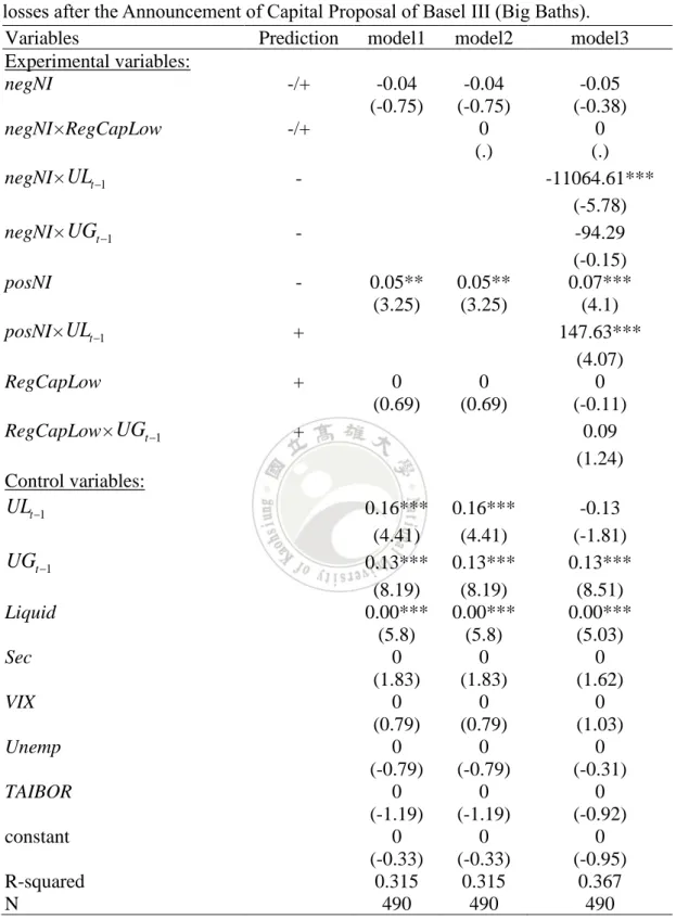
Table 10: Summary statistics from regressions of realized AFS securities gains and losses after the Announcement of Capital Proposal of Basel III (Big Baths). ... 37

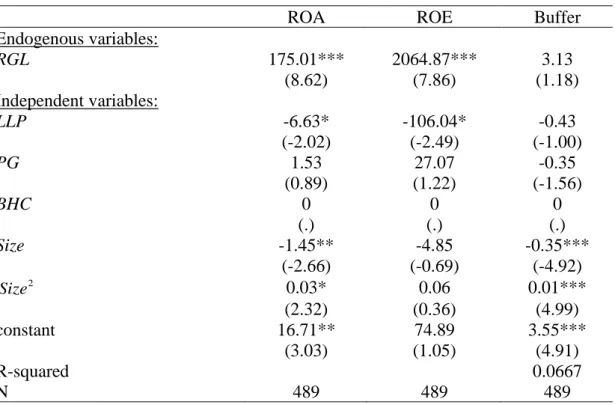
Table 11: Summary statistics from two-stage least squares regression to estimate the long-term performance of banks before the Announcement of Capital Proposal of Basel III. ... 40

Table 12: Summary statistics from two-stage least squares regression to estimate the long-term performance of banks after the Announcement of Capital Proposal of Basel III. ... 40

(7)

Chapter 1 Introduction

1 Introduction

In accounting, earnings management is the alternative accounting methods to make financial statements look better. When companies can incur expenses and recognize revenue, earnings management takes advantage of how accounting rules can be applied. Earnings management can be regarded as the results of the flexibility of accounting principles. In general, banks manipulate their earnings by using loan loss provisions or realizing security gains or losses to window dressing their income statements. Schipper (1989) and Healy and Wahlen (1999) stated that earnings management was the alteration of firms reported economic performance by insiders to either ‘‘mislead some stakeholders’’ or to ‘‘influence contractual outcomes’’. However, financial institutions, including commercial banks, are often excluded from the research of corporate earnings management because characteristics of financial institutions differ fundamentally from corporations (Peasnell et al., 2000).

The banking industry is highly regulated and is subject to government policies. Compared to corporations, banks might have less opportunities to manipulate their earnings. The approaches for managing earnings in banks might be different from those in corporations. Most of the existing literature in banking has focused on loan loss provisions (LLPs) or loan loss reserves as proxies for earnings management. Some studies find that banks use the loan loss provision to manage regulatory capital (Moyer 1990; Beatty et al. 1995; Ahmed et al. 1999; Pérez et al. 2008). However, there are few studies pay attention to available-for-sale (AFS) securities as a tool for earnings management in banks. Therefore, the objective of this study is to examine the earnings management of banks by using AFS securities.

(8)

After December 15, 1993, FASB Accounting Standards Codification (ASC) Topic 320 categorizes firm investments in three categories. They are held-to-maturity securities, trading securities, and available-for-sale securities. Held-to-maturity securities are the securities that firms have the positive intent and ability to hold to maturity. Those securities are reported at amortized cost. Trading securities are the securities that are bought and held principally for the trading purpose in the near term. Those are reported at fair value and the unrealized gains and losses are included in earnings. Available-for-sale (AFS) securities are the securities which are not classified as either held-to-maturity securities or trading securities. They are also reported at fair value, but the unrealized gains and losses of AFS securities are excluded from earnings and reported in a separate component of shareholders' equity.

In general, existing literatures use loan loss provisions (LLPs) as the proxy of earnings management of the banking industry. LLPs are the accounting items in the income statements and reflect the probability of future losses from defaults on outstanding loans. The recording of LLPs reduces net income. Commercial bank regulators view accumulated LLPs, the loan loss allowance account on the balance sheet, as a type of capital that can be used to absorb losses. In addition, banks can use LLPs to smooth bank earnings and affect bank capital through the adjustment of the earnings. However, there is alternative that banks can use the AFSs to prevent the fluctuation of the earnings. Furthermore, AFS securities can affect bank capitals without influencing the earnings. Nissim and Penman (2007) and Laux and Leuz (2010) report that banks classify 95% of non-trading securities as AFS, which represents 16% of total assets. Therefore, change of AFS securities as the proxy of earnings management can be an alternative approach for banks to manipulate their earnings and capital. Moreover, Basel III requirement more banks capitals in terms of quantity and quality. Banks have

(9)

more incentives to increase their AFS securities to manipulate capital without affecting their earnings. Hence, this study mainly focuses on the use of AFS securities to investigate the influence on earnings management. Barth et al. (2017) find robust evidence that banks realize gains and losses on AFS securities to smooth earnings and regulatory capital. Before FASB Accounting Standards Codification (ASC) Topic 320, the unrealized gains and losses of AFS securities have no recognition in the financial statement based on their fair market values.1_{ASC 320 starts measuring AFS securities} at market fair value in the statement of financial positions and excluding the unrealized gains and losses from earnings. The unrealized gains and losses of AFS securities are reported in a separate component of shareholders' equity recognizing.

The International Accounting Standard 39 (IAS 39) Financial Instruments, issued by International Accounting Standards Board (IASB) in December 1998, is effective in January 2001. The Taiwan government take IAS39 to specify the recognition and the measurement. At present, the main specification of the bulletin for the recognition and measurement of financial instruments in Taiwan is at TW GAAP 34. Since the bulletin is initially set out in accordance with IAS 39 and has been revised several times, there is little difference between the contents. However, the Taiwan Domestic bulletin provides that the evaluation of financial products basically takes the fair value evaluation, if there is no clear fair value by cost evaluation. Therefore, the company is currently in the non-active market bonds and unlisted shares of the company, are recognized at the purchase cost. Unless there are signs of significant impairment, still recognized as the original cost. In contrast, according to IAS 39, even if the equity instrument is in non-active market, its fair value should be measured at fair value.

1_{FASB Accounting Standards Codification (ASC) Topic 320 (formerly Statement of Financial} Accounting Standards No. 115, FASB 1993) created AFS securities and specified a new accounting

(10)

Therefore, there will be a difference in the accounting treatment of financial assets at the cost of domestic companies in Taiwan. For the part of the financial assets measured at cost, it is basically expected that the general business will be adjusted after the application of IAS 39. Compared to ASC 320, IAS 39 applies to a looser set of financial instruments. IAS 39 defined AFS securities are measured at fair value in the balance sheet. Fair value changes on AFS securities are recognized directly in equity, through the statement of changes in equity. Moreover, on 24th_{, July 2014, International Financial} Reporting Standard 9 (IFRS 9) Financial Instruments be issued, replacing IAS 39 requirements for classification and measurement, impairment, hedge accounting and stopping recognition. IFRS 9 is effective for annual periods beginning on or after 1 January 2018. IFRS 9 eliminates the available for sale (AFS) category, and it also eliminates the AFS impairment rules.

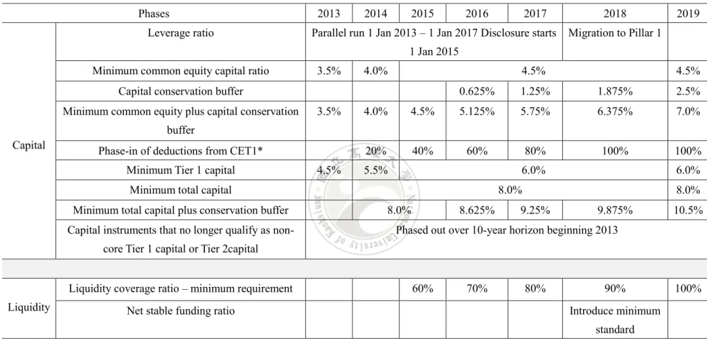
After the financial crisis of 2007-2009, Bank of International Settlements (BIS) establishes more strict regulations on Basel Accord. One of the important issues of Basel III emphasizes on minimum capital requirements shown in Table 1. The minimum requirement of Tier 1 capitals will increase from 4.5% to 6% from 2013 to 2019 to ensure the operating capacity of banking institutions. The banks should maintain the BIS ratio at least 8% with 2.5% capital conservation buffer. Therefore, the official implementation of Basel III after 2019 will require the BIS ratio up to 10.5%. The capital requirement of Basel III can improve not only the quantity but also the quality of banks’ capitals. However, it raises the costs of banks’ capital and operation. Increasing capital might also dilute the earnings per share of banks. Therefore, banks might have incentives to maintain their earnings during the transition periods of Basel III from 2013 to 2019. This study adopts the unrealized gains and losses of AFS securities as the proxy to examine the earnings management behavior of banks.

(11)

Furthermore, this study tests the effects of earnings management on bank long-term performance.

The objectives of this study are to use AFS securities as a proxy to discuss the impacts of earnings management on banks. Furthermore, this study analyzes the bank’s capital adequacy ratio and long-term performance affected by earnings management. The results can be the evidence that whether IFRS 9 Financial Instruments, which is officially effective on 2018, is appropriate for eliminating AFS securities in the banking industry to replace IAS 39.

The remainder of the paper proceeds as follows. Section 2 reviews the literature on earnings management and previous studies shown to be important in other contexts. Section 3 describes the data and methodology. Section 4 describes the empirical results and Section 5 concludes the paper.

(12)

Table 1: Basel III Phase-in Arrangements

Phases 2013 2014 2015 2016 2017 2018 2019

Capital

Leverage ratio Parallel run 1 Jan 2013 – 1 Jan 2017 Disclosure starts

1 Jan 2015

Migration to Pillar 1

Minimum common equity capital ratio 3.5% 4.0% 4.5% 4.5%

Capital conservation buffer 0.625% 1.25% 1.875% 2.5%

Minimum common equity plus capital conservation buffer

3.5% 4.0% 4.5% 5.125% 5.75% 6.375% 7.0%

Phase-in of deductions from CET1* 20% 40% 60% 80% 100% 100%

Minimum Tier 1 capital 4.5% 5.5% 6.0% 6.0%

Minimum total capital 8.0% 8.0%

Minimum total capital plus conservation buffer 8.0% 8.625% 9.25% 9.875% 10.5%

Capital instruments that no longer qualify as non-core Tier 1 capital or Tier 2capital

Phased out over 10-year horizon beginning 2013

Liquidity

Liquidity coverage ratio – minimum requirement 60% 70% 80% 90% 100%

Net stable funding ratio Introduce minimum

standard

Including amounts exceeding the limit for deferred tax assets (DTAs), mortgage servicing rights (MSRs) and financials. All dates are as of 1 January

(13)

Chapter 2 Literature Review

2 Literature review

Earnings management is the alternative accounting methods used by the management of a company to manipulate their company’s earnings. The management of a company can control their company’s earnings through smoothing earnings, managing earnings relative to a pre-determined target or taking a big bath. When the managers of the company conduct earnings management, it can window dressing their income statements, revealing a relatively stable financial performance of a company. Furthermore, earnings management may mislead some stakeholders or financial analyst’s opinions about future outcomes of securities in the form of earnings. Therefore, considerable study on earnings management has been done and provides motivations and evidences for a manager to manage earnings.

2.1 Related studies on earnings management

2.1.1 Earnings management in Corporate

Earnings is regarded as one of the most important factor of a firm. It is not only draw the attention of academic researchers but also the financial market regulator, operator, investor follow it with interest. Previous studies have mainly focused on incentives of earnings management. Healy (1985) and Guidry (1999) both find the evidence that the manager tends to manipulate earnings to maximize their short-term bonus plans with the level of business units and aggregate firm respectively. Teoh et al. (1998a) state that IPO issuers in the most “aggressive” quartile of earnings managers have a three-year aftermarket stock return of approximately 20 percent less than IPO issuers in the most “conservative” quartile. Healy and Wahlen (1999) and Dechow et al. (2010b) were on smoothing earnings. Dechow et al. (2010a) recognize large losses

(14)

when a loss is unavoidable to increase the likelihood of positive earnings in the future. Coppens and Peek (2005), Graham et al. (2005), Burgstahler et al. (2006), and Hope et al. (2013) reveal that non-listed firms also perceive earnings management as important. Schilit (2001) states that Earnings Smoothing is when the managers will use the method of expanding current revenues and gains or deducting current expenses to inflate the current surplus, which can achieve the purpose of window dressing the financial statements. Taking a big baths is when the managers will use the method of deducting revenues or expanding current expenses to deflate the current surplus, which shift the surplus to the future and realize the surplus when it is needed.

2.1.2 Earnings management in Bank

These incentives in previous paragraph can also apply to banking industry. Many studies have investigated whether bank managers use their discretion to manager reported earnings and identify the method used to manage earnings. Previous studies pay the most attention on income smoothing and focus on the use of LLPs for earnings management.

Beatty et al. (2002) find that relative to private banks, public banks are more likely to use loan loss provisions and realized securities gains and losses to eliminate small earnings decreases. Thus, opportunistic earnings management by banks does indeed appear to be accomplished through the recording of loan loss provisions and realization of securities gains and losses. Arya et al. (1998) and Demski (1998) find earnings management can be used to discreetly smooth earnings over time or to eventually and indiscreetly take a big bath, that is, report one drastic earnings decline after hiding a series of smaller declines in previous years. Kanagaretnam et al. (2004) find that banks use discretionary LLP to smooth income but not to signal private information.

(15)

Anandarajan et al. (2007) suggest that publicly traded commercial banks in Australia engage in earnings management practices. Pérez et al. (2008) show evidence for income smoothing using 142 Spanish banks from 1986 to 2002. Leventis et al. (2012), using a sample of 91 EU banks, conclude that income smoothing is more pronounced among risky banks but this smoothing behavior is less aggressive after implementation of IFRS. In a US study, Balboa et al. (2013), using 9442 US banks from 1999 to 2008, find evidence for income smoothing but believe that this relationship may be driven by non-linear patterns. Curcio and Hassan (2015) find strong evidence for income smoothing among non-EU credit institutions. However, some studies show conflicting evidence. Wetmore and Brick (1994) and Ahmed et al. (1999) find no evidence to support the income smoothing hypothesis after the implementation of Basel I.

Overall, the literature documents more positive evidence of smoothing via LLP. However, neither of them follow AFS with interest. To my knowledge, there are only two previous study reporting evidence of banks using realized AFS securities gains and losses to smooth earnings. One is Lifschutz (2002), the other is Barth et al. (2017).

Lifschutz (2002) estimates the relation between (i) the ratio of realized securities gains and losses to total value of AFS securities and (ii) return on equity or return on assets and concludes that the motivation of managers of these banks to manage earnings by realizing securities gains and losses is negatively related to bank earnings before realized gains and losses. Based on a large sample of publicly listed and non-listed US commercial banks from 1996 to 2011, Barth et al. (2017) find robust evidence consistent with banks using realized available for sale (AFS) securities gains and losses to smooth earnings and increase low regulatory capital. Barth et al. (2017) also state that (i) banks with positive earnings smooth earnings, and banks with negative earnings

(16)

generally take big baths2_{; (ii) regulatory capital constrains big baths, (iii) banks with} more negative earnings and more unrealized beginning-of-quarter losses (gains) take big baths (smooth earnings); and (iv) banks with low regulatory capital and more unrealized gains realize more gains.

In short, previous two studies suggest banks use realized available for sale (AFS) securities gains and losses to smooth earnings. We revisit this question by using realized available for sale (AFS) securities gains and losses to smooth earnings with bank’s capital adequacy ratio and bank’s long term performance and hope this feature could enable us to provide more robust evidence than in prior study.

H1: Banks use realized available for sale (AFS) securities gains and losses to

smooth earnings or take big baths that generate favorable effect of earnings management.

2.2 Earnings Management and Capital Adequacy Ratio

2.2.1 Related studies on Capital Adequacy Ratio

Capital adequacy ratios measure the amount of a bank's capital in relation to the amount of its risk weighted credit exposures. When the banks have the higher the capital adequacy ratios, it can absorb the greater the level of unexpected losses before becoming insolvent. Capital adequacy ratios is used to protect depositors and promote the stability and efficiency of financial systems around the world. Two types of capital are measured: tier one capital, which can absorb losses without a bank being required to cease trading, and tier two capital, which can absorb losses in the event of a

2_{Barth et al. (2017) define “big bath” earnings management as banks with more negative earnings before} realized AFS securities gains and losses realizing more losses or fewer gains and expect banks with negative earnings that sell AFS securities to select securities with unrealized losses or with smaller unrealized gains, thereby enhancing their ability to realize larger gains in future periods.

(17)

up and so provides a lesser degree of protection to depositors. During the process of winding-up, funds belonging to depositors are given a higher priority than the bank’s capital, so depositors can only lose their savings if a bank registers a loss exceeding the amount of capital it possesses. Therefore, the higher the bank’s capital adequacy ratio, the higher the degree of protection of depositor's money. The Basel Capital Accord is an international standard for the calculation of capital adequacy ratios. The Accord recommends minimum capital adequacy ratios that banks should meet. Under Basel III, the minimum capital adequacy ratio that banks must maintain is 8%. The capital adequacy ratio measures a bank's capital in relation to its risk-weighted assets. The capital to risk-weighted assets ratio promotes financial stability and efficiency in economic systems throughout the world.

2.2.2 Earnings Management and Capital Adequacy Ratio

The capital adequacy of a bank shall be determined based on the basis of a bank’s Regulatory Capital. Berger et al. (1995) state Bank capital regulation is intended to mitigate moral hazard problems that arise from the provision of deposit insurance, lender-of-last resort facility, and other guarantees by the government. The banks are subject to regulatory capital requirements and so that banks with low regulatory capital have an incentive to increase it or at least not decrease it substantially. For the reason that, banks could manage earnings to accomplish the purpose. Beatty and Liao (2014) provides a review of the large empirical literature on the banking industry, including that addressing earnings management.

Moyer (1990) finds the inclusion of loan loss reserves in defining regulatory capital implied that a one dollar increases in the loan loss provision increased regulatory capital by the tax rate times one dollar. Therefore, managers of banks with low regulatory capital had incentives to increase loan loss provisions. Moyer (1990) also

(18)

finds evidence consistent with banks using realized securities gains and losses to increase regulatory capital, but only for banks with regulatory capital below the minimum. Scholes et al. (1990) finds a significant negative relation between banks’ regulatory capital and realized securities gains and losses, which suggests banks use realized securities gains and losses to smooth regulatory capital. Beatty et al. (1995) finds a negative relation between miscellaneous gains and losses and regulatory capital, although the relation is not significantly negative in all specifications. Collins et al. (1995) finds that after 1980 realized securities gains and losses are not consistently negatively related to regulatory capital.

H2: Banks use low regulatory capital realize more gains for managers have

incentives to manage earnings.

2.3 Earnings management and Performance

2.3.1 Related studies in Corporate

From the point of view of a firm, it is important to understand the methods of earnings management because firm performance relies on net income and managers can manipulate net income through current assets. Earnings management is done by affecting total accruals and discretionary accruals.

Richardson et al. (2006) find that accruals are associated with earnings manipulation. Sloan (1996) finds that the accrual component of operating income is less persistent than the cash components for explaining one-year-ahead performance measured by the rate of return on assets (ROA). Fairfield et al. (2003), by sampling US firms for a period of 1963-1992 find that working capital accruals have a negative relation with future profitability. Working capital accruals include current assets and

(19)

current liabilities. Fama and French (2006) analyze data of US firms and find that accruals negatively predict one-year-ahead reported profitability. Cooper et al. (2008), sampling US firms for a period of 1963-2003, find a negative correlation between total asset growth and subsequent firm abnormal returns. Chu (2012), analyzing a sample of 4,438 US firms for a period of 1978-2007, find that high growth firms with low accruals experience high future profitability and returns.

There are some motivations behind earnings management. One of the motivations is to provide good news to corporate boards by showing good results in a certain period. Cohen et al. (2011) finds managers are reluctant to announce earnings below analysts’ forecasts because it may have a negative impact on market price per share. Because market price per share impacts the value of the firm, managers tend to manipulate the components of the income statement and balance sheet through accruals to maintain and/or to maximize share price for the current and subsequent year. However, earnings manipulation tends to start backfiring after some time.

For example, Teoh et al. (1998), sampling 1,649 US initial public offering (IPO) firms from 1985-1992, find that issuers with unusually high accruals in the IPO year experience poor stock return performance in the three years thereafter. Managers also tend to manipulate earnings to surprise investors, improve share price, and lower debt costs. DuCharme and Malatesta (2004), sampling US companies for the period of 2000-2001, find that abnormal stock returns are positively related to the earnings surprise. Othman et al. (2009), using data from US COMPUSTAT for a period of 1984-1999, find that earnings management positively impact market price per share and led to the 1990s stock market bubble. Li (2010) sampling of 7,861 US firms for the period 1988-2008, find that real earnings management practices of managers are related to subsequent higher stock returns. Gholami et al. (2012) sampling 1,200 US IPO firms

(20)

for the period of 2000-2010. They find that IPO firms engaged in earnings management with high investor beliefs have an influence on the long-run abnormal stock return performance. Mahdi et al. (2012) and Rahmani and Akbari (2013) examine the effective variables on earnings management. By using the multiple correlation analysis, the study documented that there exist negative association between performance coefficient and earnings management while positive relation between firm’s size with earnings management. Ali et al. (2015) observe negative relation but Bassiouny et al. (2016) observed no significant association.

2.3.2 Related studies in Bank

The reason for earnings management is takes advantage of the different ways that accounting policies and procedures can be applied to financial reporting. Earnings management seems to turn some management ways that illegal to legal, by using window dressing, internal targets, income smoothing, external expectations. Window dressing refers to the company’s decision to dress up the financial statements for potential investors and creditors. The goal of this is to attract new supporters by having well-doing financial statements. Internal targets are another reason that a company may choose to use earnings management techniques. The company has set its own internal goals, such as departmental budgeting, and wants to be sure to meet those goals. Income smoothing comes into play here because of the fact that potential investors generally like to invest in companies that have a continuous growth pattern. External expectations come into play when the company has already made projections as to what their profits will be reach and investors now expect that exact amount of profits or more. Management may feel the need to shift revenue from one accounting period to another in order to meet the projected goal. Therefore, Suda and Shuto (2006) state companies will engage in earnings management when the benefits of this behavior are higher than

(21)

the risks and costs involved.

Prior studies are mainly focused on the main idea of what is bank earnings management and measurement on the earnings management. As time goes on, the earnings of bank industry and regulatory capital management ability are changed. Because the capital requirement of Basel III can improve not only the quantity but also the quality of banks’ capitals, the cost of capital for operating a bank is increasing. Therefore, bank might have the incentives to manage the earnings management to smooth the impact of the increasing costs of capital.

2.4 Capital Adequacy Ratio and Bank Performance

Capital as an important factor of production must be sufficient in business for effective operation of an organization. Bank is one of these organizations whose capital adequacy is of paramount significance to its customers. Barrios and Blanco (2000) state Capital accounts form a small percentage of the financial resources of the banking institutions and it plays a crucial role in their long-term financing and solvency position. Furlong and Keeley (1991) list the factors that may affect bank’ s capital; these include competition, more depositors, less fund costs, risk in portfolio interest, high return on equity, less distress incidences, profit maximization, avoidance of bankrupt and their negative externalities on the financial system and incentive to increase risky assets. The effect of capital adequacy on bank’ s performance depends highly on these factors and the regulatory body prevailing in the country. Because the bank’s capital, accounts for over 30% and 44% of the banks’ total assets and deposits, determining capital adequacy of banks might be misleading. Therefore, Barrios and Blanco (2000) state that determining bank’s performance in relation with its capital adequacy and some variables must be considered. These variables include managerial quality of the bank

(22)

and productive efficiency which depends on the degree of competition in the industry. The ability of the bank management to ensure that bank’s capital is effectively managed, determines how adequate the capital is. Having capital adequacy ratios above the minimum levels recommended by the Basle Capital Accord, does not guarantee safety of a bank, as capital adequacy ratios is concerned primarily with credit risks. As Brash (2001) observe that “there are also other types of risks which are not recognized by capital adequacy ratios, for example: inadequate internal control systems could lead to large losses by fraud, or losses could be made on the trading of foreign exchange and other types of financial instruments”. Other risks involved in financial transitions must be view as relevant while determining bank performance. In other words, Brash (2001) state capital adequacy ratios are only as good as the information on which they are based and should not be interpreted as the only indicators necessary to judge a bank’ s financial soundness.

(23)

Chapter 3 Data and Methodologies

3.1 Data Source

This study bases the sample on all commercial banks and bank holding companies in Taiwan of Taiwan Economic Journal Database, to investigate Taiwan commercial bank’s earnings management on Bank Capital Adequacy and Long-term Performance affected by Available for Sale Securities. The sample of examination periods is from September, 2008 to September, 2017 and the sample begins in September, 2008 because Taiwan officially starts to take IAS 39, which is TW GAAP 34 of Taiwan Domestic bulletin. The period includes 2008 and 2009, which is the year that financial crisis happened. Therefore, this study uses the dummy variables to avoid the potential for the financial crisis to affect our inferences. Besides, in order to investigate the effect of the government taking Basel III, this study also tests the separated period in 2008 to 2012 and 2013 to 2017. The resulting sample comprises 38 banks of Taiwan.

3.2 Variables

The dependent variable of this study is Realized gains and losses on available for sale (AFS) securities, deflated by beginning-of-quarter total assets. Realized gains and losses on AFS securities, RGL, comprises gains and losses realized by sale or other disposal of the securities and losses arising from other than temporary impairment (OTTI) of the securities. Realized income or losses are recorded on the Income statement by IFRS 9, therefore, gains and losses from transactions that have been completed and recognized. Consequently, this study uses RGL to test whether banks smooth earnings and regulatory capital or engage in a big bath for managing earnings.

(24)

According to IFRS 9, eliminates the available for sale (AFS) category, it also eliminates the AFS impairment rules. Under IAS 39 measuring impairment losses on debt securities in illiquid markets based on fair value often led to reporting an impairment loss that exceeded the credit loss management expected. The unrealized gains and losses on AFS securities are excluded from Tier 1 regulatory capital and only affect when they are realized. However, there are 45% of unrealized gains and losses an AFS equity securities included in Tier II capital. Therefore, Basel III Capital Accord requires banks to hold enough quality assets to meet the liquidity coverage ratio needs. Banks concern about liquidity risk may be attracted to securities because securities of banks can more easily be sold and with lower price impact than loans.

Moreover, the banking industry is typically sensitive to the cyclical movements of economy. The cyclical movements of economy can affect both the market for bank credits and the probability. Prior studies test banks’ behavior influenced by macroeconomic conditions and through using AFS securities to smooth earnings and take a big bath. Richard and Menghistu (2014) state many US banks use AFS securities to smooth their earnings during the most macroeconomic business cycle from 2001 to 2010. As well as, the evidence find US banks are more likely to smooth income when the general macroeconomic environment is favorable.

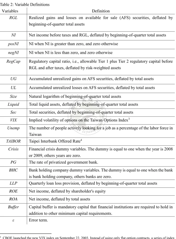
As a result of above reasons, this study uses the independent variables that include Net income before taxes and RGL, deflated by beginning-of-quarter total assets (NI), Accumulated unrealized gains or losses on AFS securities, deflated by total assets (UG,UL), Total securities, deflated by total assets (Sec), Natural logarithm of beginning-of-quarter total assets (Size), Total liquid assets, deflated by total assets (Liquid), and macroeconomic controls. Table 2: Variable Definitions shows the summary of the both independent and dependent variables

(25)

Table 2: Variable Definitions

Variables Definition

RGL Realized gains and losses on available for sale (AFS) securities, deflated by beginning-of-quarter total assets

NI Net income before taxes and RGL, deflated by beginning-of-quarter total assets

posNI NI when NI is greater than zero, and zero otherwise

negNI NI when NI is less than zero, and zero otherwise

RegCap Regulatory capital ratio, i.e., allowable Tier 1 plus Tier 2 regulatory capital before RGL and after taxes, deflated by risk-weighted assets

UG Accumulated unrealized gains on AFS securities, deflated by total assets

UL Accumulated unrealized losses on AFS securities, deflated by total assets

Size Natural logarithm of beginning-of-quarter total assets

Liquid Total liquid assets, deflated by beginning-of-quarter total assets

Sec Total securities, deflated by beginning-of-quarter total assets

VIX Implied volatility of options on the Taiwan Options Index3

Unemp The number of people actively looking for a job as a percentage of the labor force in Taiwan

TAIBOR Taipei Interbank Offered Rate4

Crisis Financial crisis dummy variables. The dummy is equal to one when the year is 2008

or 2009, others years are zero.

PG The rate of privatized government bank.

BHC Bank holding company dummy variables. The dummy is equal to one when the bank

is bank holding company, others banks are zero.

LLP Quarterly loan loss provision, deflated by beginning-of-quarter total assets

ROE Net income, deflated by shareholder's equity ROA Net income, deflated by total assets

Buffer Capital buffer is mandatory capital that financial institutions are required to hold in

addition to other minimum capital requirements.

ε Error term.

3_{CBOE launched the new VIX index on September 22, 2003. Instead of using only flat option contracts, a series of index} options with different strike prices can be used to calculate the expected volatility.

(26)

3.3 Methodologies

3.3.1 Smooth earnings and Regulatory capital

To determine whether banks use realized gains and losses on AFS securities to smooth earnings and whether banks with regulatory capital decrease the volatility of earnings. All of the panel regression models in this study with bank fixed effect is used to estimate the earnings smoothing and employ residual standard errors clustered by bank and year-quarter to construct t-statistics. Moreover, the regression analysis to test earnings smoothing hypothesis will be divide into two stages which are the year before the announcement of capital proposal of Basel III from year 2008 to 2012 and after the announcement of capital proposal of Basel III from 2013 to 2017.

0 1 2 3 1 1 2 1 3 4 5 6 7 8 + + it it it it it it it it t t t t it RGL NI RegCapLow NI RegCapLow UL UG Liquid Sec VIX Unemp TAIBOR Crisis

     

      

− −

= +  + +

+ + + + + + + (1)

where in equation (1) includes the main independent variables such as NI and

RegCapLow and it also has UL, UG, Liquid, and Sec as controls for bank characteristics

likely associated with realized gains and losses on AFS securities. In addition, equation (1) includes macroeconomic control variables because securities gains and losses likely depend on economic condition such as VIX, Unemp, TAIBOR, and Crisis.

RGL is realized gains and losses on AFS securities and NI is net income before taxes and RGL, both deflated by beginning-of-quarter total assets. RegCapLow is an indicator variable that equals one if the bank’s regulatory capital ratio—which bank regulators define as allowable Tier 1 plus allowable Tier 2 regulatory capital, deflated by risk-weighted assets—before RGL and after taxes, is in the lowest decile for the

(27)

quarter, and zero otherwise.

UG is accumulated unrealized gains on AFS securities, UL is accumulated

unrealized gains and losses on AFS securities. Liquid is the sum of cash items in process of collections. Sec is the sum of held-to-maturity, available-for-sale, and trading securities. The variables of UG, UL, Liquid, and Sec are deflated by beginning-of-quarter total assets. VIX is implied volatility of options on the Taiwan Options Index.

Unemp is the number of people actively looking for a job as a percentage of the labor

force in Taiwan. TAIBOR is Taipei Interbank Offered Rate. Crisis is financial crisis which occured in 2008 and 2009. These variables are quarterly, which eliminates need to include quarter fixed effects. ε is error term. The terms i and t denote bank and period.

If banks attempt to perform smoothing earnings, this study predicts there will have a negative relationship within RGL and NI whereas positive relationship within RGL and RegCapLow. The relationship within RGL and interaction variables

NI×RegCapLow depends on whether earnings smoothing is dominated by positive or

negative NI banks. If it is dominated by positive NI banks recognizing more losses or fewer gains, then the relationship is positive. On the other hands, if it is dominated by negative NI banks recognizing fewer losses or more gains, then the relationship is negative. In this study excepts bank with more unrealized gains and losses are more likely to realize them to smooth earnings.

3.3.2 Engage in a big bath for managing earnings

To determine whether banks with negative earnings use realized AFS securities losses and gains to engage in big bath for managing earnings if their unrealized gains are insufficient to offset the negative earnings. Therefore, this study proceeds to expand equation (1) by separating negative and positive NI banks and to determine whether

(28)

banks with negative NI realize fewer losses or more gains, which is consistent with earnings smoothing, or whether they realize more losses or fewer gains, which is consistent with taking a big bath. In other words, this study expects banks with positive

NI to smooth earnings. Equation (2) uses panel regression models with bank fixed effect

is used to estimate big bath earnings management. The regression analysis to test earnings smoothing hypothesis will be divide into two stages which are the year before the announcement of capital proposal of Basel III from year 2008 to 2012 and after the announcement of capital proposal of Basel III from 2013 to 2017.

0 1 2 3 1 4 1 5 6 1 7 8 1 1 1 2 1 3 4 5 6 + + it it it it it it it it it it it it it it it it it it t

RGL negNI negNI RegCapLow negNI UL negNI UG B posNI posNI UL RegCapLow RegCapLow UG

UL UG Liquid Sec VIX U

              − − − − − − =  +  +  + +  + + 

+ + + + + + nemp_t+ ₇TAIBOR_t+ ₈Crisis_t+ _it

(2)

where in equation (2) includes the main independent variables such as negNI, posNI,

RegCapLow, UG, UL, Size, Liquid, and Sec. posNI (negNI) is NI if NI is greater (less)

than zero, and zero otherwise. The macroeconomic control variables which are VIX,

Unemp, TAIBOR, and Crisis that similar to earnings smoothing model.

If bank with negative NI take a big bath (smooth earnings), this study predicts that there will have a positive (negative) relationship for RGL and negNI. Low regulatory capital provides incentives to realize more gains, which mitigates the incentive for negative NI banks to take big baths. Thus, this study predicts that there will have negative relationship within RGL and negNI×RegCapLow. Because there is more opportunity for big bath earnings management when negative NI banks have more accumulated unrealized losses, this study predicts that there will have negative relationship for RGL and negNI×ULt−1. Because there is more opportunity for earnings

smoothing when negative (positive) NI banks have more accumulated unrealized gains (losses), this study predicts that there will have negative (positive) relationship for RGL

(29)

and negNI×UGt−1 (posNI×ULt−1). Because there is more opportunity to realize gains

to increase regulatory capital when the bank has more accumulated unrealized gains, this study predicts that there will have a positive relationship for RGL and

RegCapLow×UGt−1. All other predictions are as in equation (1).

3.3.3 Long-term performance

To determine whether the return on assets (ROA) of banks, the return on equity (ROE), and capital buffer (Buffer) affect the long-term performance. The two-stage least squares (2SLS) regression model in this study with bank fixed effect is used to estimate the long-term performance. The regression analysis to test earnings the long-term performance of banks will also be divide into two stages which are the year before the announcement of capital proposal of Basel III from year 2008 to 2012 and after the announcement of capital proposal of Basel III from 2013 to 2017.

2

0 + 1 + 2 3 4 5 6

it it it it it it it it

ROA =   RGL  LLP +  PG +  BHC +  Size +  Size +  (3)

2

0 + 1 + 2 3 4 5 6

ROE =   RGL  LLP +  PG +  BHC +  Size +  Size +  (4)

2

0 + 1 + 2 3 4 5 6

Buffer =   RGL  LLP +  PG +  BHC +  Size +  Size +  (5)

where in equation (3) 、(4) 、(5) includes the main dependent variables are similar as equation (2). The NI variable is divided into negNI and posNI. The RGL is endogenous variable. The negNI, posNI, RegCapLow, UG, UL, Size, and Liquid are instrumental variables. The VIX, Unemp, TAIBOR, and Crisis are macroeconomic control variables.

(30)

Chapter 4 Results and Discussions

4.1 Descriptive Statistics

The samples of this study are from all commercial banks and bank holding companies in Taiwan of Taiwan Economic Journal Database to examine the earnings management of banks. The periods of sample contain September, 2008 to September, 2017. The sampling periods contain 2008 and 2009 even though the financial crisis happened at that time. The macroeconomic variables such as VIX is from Taiwan Futures Exchange, Unemp is from Nation Statistics of Taiwan, and TAIBOR is from The Bankers Association of Taiwan. Because of the availability of the data of realized and unrealized gains and losses of AFS securities, there are 1185 bank-quarter observations for 38 banks available tested in the models.

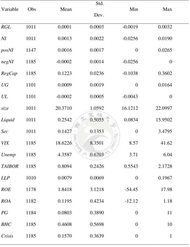
Table 3 shows the summary statistics of the variables in this study. In this table, it shows banks realize gains on AFS securities (mean RGL= 0.0001; std. dev. = 0.0003) net income before realized gains and losses on AFS securities (NI) is also positive (mean = 0.0013; std. dev. = 0.0022) Furthermore, net income deflated by beginning-of-quarter total assets is divided into two categories, which are positive net income (posNI) and negative net income (negNI). The value of posNI is equal to NI when NI is positive but it is zero when NI is negative. Simultaneously, the value of negNI is equal to NI when NI is negative but it is zero when NI is positive. Means (Std. dev.) of positive and negative NI, posNI and negNI, are 0.0016 and -0.0002 (0.0017 and 0.0014). Mean (Std. dev.) of regulatory capital ratio before realized gains and losses on AFS securities, which this study uses to construct RegCapLow is, 0.1223 (0.0236). Means (std. dev.) of banks’ accumulated unrealized gains and losses on AFS securities, UG and UL, are

(31)

0.0009 and -0.0002 (0.0019 and 0.0005). Table 3 also shows the macroeconomic variable, mean (std. dev.) of the implied volatility of options on the Taiwan Options Index (VIX) is 18.6226 (8.3501), unemployment rate of Taiwan’s labors (Unemp) is 4.3587 (0.6703), and Taipei Interbank Offered Rate (TAIBOR) is 0.8094 (0.2426).

Table 4 shows Person/Spearman correlation matrix of the variables. The lower left is the Pearson correlation coefficients and the upper right is the Spearman correlation matrix. Table 4 shows RGL is significantly positively related to NI (Pearson corr. = 0.2651; Spearman corr. = 0.2216). This study predicts when the correlation of NI is negative, the Banks tend to use AFS securities gain and losses to smooth earnings. Conversely, when the correlation of NI is positive, the Banks tend to use AFS securities gain and losses to take big baths that generate favorable effect of earnings management. From Pearson correlation matrix, the correlations of Size, VIX, TAIBOR, PG, BHC and

Crisis have negative relationship with RGL whereas the others have positive

relationship with RGL. In this table, most of the correlations are significantly different from zero and the star is significant values at 5%. Therefore, this study uses regressions to test the predictions.

(32)

Table 3: Descriptive statistics

Variable Obs Mean

Std. Dev. Min Max RGL 1011 _0.0001 _0.0003 _-0.0019 _0.0032 NI 1011 _0.0013 _0.0022 _-0.0256 _0.0190 posNI 1147 _0.0016 _0.0017 0 _0.0265 negNI 1185 _-0.0002 _0.0014 _-0.0256 0 RegCap 1185 _0.1223 _0.0236 _-0.1038 _0.3602 UG 1101 _0.0009 _0.0019 0 _0.0164 UL 1101 _-0.0002 _0.0005 _-0.0043 0 size 1011 _20.3710 _1.0592 _16.1212 _22.0997 Liquid 1011 _0.2542 _0.5055 _0.0834 _15.9502 Sec 1011 _0.1427 _0.1353 0 _3.4795 VIX 1185 _18.6226 _8.3501 8.57 41.62 Unemp 1185 _4.3587 _0.6703 3.71 6.04 TAIBOR 1185 _0.8094 _0.2426 _0.5543 _2.1728 LLP 1010 _0.0079 _0.0069 0 _0.1967 ROE 1178 _1.8418 _3.1218 _-54.45 17.98 ROA 1182 _0.1195 _0.4234 _-12.12 1.18 PG 1184 _0.0803 _0.3890 0 11 BHC 1185 _0.4608 _0.5698 0 10 Crisis 1185 0.1570 0.3639 0 1

(33)

Table 4: Correlation matrix

RGL NI posNI negNI RegCap UG UL Size Liquid Sec VIX Unemp TAIBOR LLP ROE ROA PG BHC Crisis RGL 1 0.2216* 0.2218* 0.1548* 0.1624* 0.2593* 0.145* 0.1344* -0.0217 0.0521 0.0071 0.0235 -0.1425* -0.0488 0.2141* 0.2256* -0.0619 0.0636 -0.0229 NI 0.2651* 1 0.9998* 0.4639* 0.3733* 0.1252* 0.1097* 0.0987* -0.032 0.1812* -0.3299* -0.3429* 0.1618* 0.0257 0.9151* 0.9787* -0.16* 0.1228* -0.3812* posNI 0.3539* 0.7523* 1 0.463* 0.3753* 0.1256* 0.1103* 0.0975* -0.0304 0.1781* -0.3292* -0.3418* 0.1617* 0.029 0.915* 0.9787* -0.1613* 0.1248* -0.3794* negNI 0.0568 0.774* 0.1652* 1 0.0705* 0.1082* 0.0698* 0.2528* -0.133* 0.1267* -0.2667* -0.2518* 0.0554 -0.0999* 0.4321* 0.4333* 0.0749* 0.0476 -0.3762* RegCap 0.1792* 0.1447* 0.3052* -0.0767 1 0.1289* 0.0765* 0.0534 -0.0414 0.2796* -0.21* -0.3797* -0.0354 0.0522 0.2204* 0.3825* -0.2806* 0.1835* -0.224* UG 0.2796* 0.0911* 0.1374* 0.0044 0.1474* 1 0.8225* 0.0664* 0.0397 0.0075 -0.0475 -0.0074 -0.0532 -0.0813* 0.1261* 0.1281* -0.0894* 0.1351* -0.0503 UL 0.0941* 0.0659 0.0652* 0.036 0.0341 0.1752* 1 -0.0059 0.0628* -0.0695 -0.0438 -0.018 -0.0611 -0.0032 0.1012* 0.1036* -0.0724* 0.0891* -0.0899* Size -0.0887* 0.0699* -0.0814 0.1829* 0.0135* -0.245* -0.052 1 -0.1845* 0.2197* -0.0853* -0.137* 0.0036 -0.2053* 0.1706* 0.1003* 0.0267 0.512* -0.0779* Liquid 0.0055 0.2576* 0.4237* -0.0216 -0.0472 -0.0123 0.0247 -0.1503* 1 -0.3481* 0.106* 0.17* 0.0361 -0.077* -0.0589 -0.029 -0.0796* -0.1226* 0.1548* Sec 0.0658* 0.3859* 0.4892* 0.1077* 0.1118* 0.0567 -0.0326 0.0198 0.7734* 1 -0.1807* -0.2606* -0.0148 -0.1006* 0.107* 0.1852* -0.066* 0.0587 -0.2307* VIX -0.0149 -0.3103* -0.2473* -0.2269* -0.2005* -0.0224 -0.1631* -0.074* -0.0015 -0.1152* 1 0.6386* -0.0595 -0.1242* -0.2704* -0.3295* -0.0211 -0.0002 0.4908* Unemp 0.0016 -0.3109* -0.2559* -0.2195* -0.2886* 0.034 -0.1095* -0.1144* 0.0126 -0.1566* 0.5706* 1 -0.2077* -0.1551* -0.2301* -0.3409* 0.0094 0.0128 0.5776* TAIBOR -0.0626 0.1145* 0.142* 0.0349 -0.0725* -0.0567 -0.0344* 0.0126 0.0363 -0.0007 -0.0015* -0.4849* 1 -0.0067 0.2011* 0.1584* 0.0413 0.0128 -0.3117* LLP -0.0025 0.1464* 0.3883* -0.154* 0.032* -0.0383 0.0342 -0.2239* 0.903* 0.6939* -0.0025 -0.0076 0.0344 1 -0.0168 0.0079 0.1548* -0.1991* -0.0021 ROE 0.1654* 0.8502* 0.456* 0.8345* 0.1055* 0.0772* 0.0879* 0.1631* -0.0207 0.1139* -0.3142* -0.2836* 0.0947* -0.0964* 1 0.9369* -0.101* 0.1308* -0.3576* ROA 0.2219* 0.9227* 0.5931* 0.8112* 0.1511* 0.1741* 0.0667 0.0933* -0.0088 0.1643* -0.3288* -0.3256* 0.1138* -0.113* 0.9245* 1 -0.1691* 0.1273* -0.3754* PG -0.015 -0.0896* -0.1828* 0.0416 -0.2728* 0.1311* 0.0946* 0.1824* -0.0152 -0.0397 0.1153 0.148 -0.0412 -0.0277 -0.0525 -0.0915 1 -0.3841* -0.0324 BHC -0.0039 -0.0278 -0.0025 -0.0393 0.1306* -0.0696 -0.0696* 0.4513* -0.0413 -0.0027 0.012 0.0237 -0.0056 -0.0432 0.0016 -0.0289 -0.0424 1 0.007 Crisis -0.011 -0.337* -0.2482* -0.266* -0.1878* 0.0091 -0.1769* -0.0731* 0.0126 -0.1394* 0.6027* 0.7781* -0.256* 0.0143 -0.3533* -0.3556* 0.0886 -0.0003 1

(34)

4.2 Collinearity Tests

Collinearity implies two variables are near perfect linear combinations of one another. Multicollinearity involves more than two variables. In the presence of multicollinearity, regression estimates are unstable and have high standard errors. Due to collinearities that exist among the predictors, variance inflation factors (VIF) measure the inflation in the variances of the parameter estimates. Moreover, the general rule of thumb is that VIF exceeding 4 warrant further investigation, while VIF exceeding 10 are signs of serious multicollinearity requiring correction.

Table 5 shows the collinearity tests of the variables on earning smoothing. The most of variables of VIF are less than 4 except that unemployment rate of Taiwan’s labors (Unemp) is 4.03 and the mean VIF is 1.69. As a result, multicollinearity problem does not exist in this model.

Table 5: Collinearity Tests (Earnings Smoothing)

Variable VIF 1/VIF

NI 1.36 0.7355 RegCapLow 1.23 0.81192 NI×RegCapLow 1.12 0.89112 1 t UL₋ 1.17 0.85244 1 t UG₋ 1.26 0.79452 Liquid 1.15 0.87139 Sec 1.28 0.77955 VIX 1.92 0.52086 Unemp 4.03 0.24844 TAIBOR 1.66 0.60228 Crisis 3.04 0.3287 Mean VIF 1.69

(35)

Furthermore, Table 6 shows the collinearity tests of the variables on taking big baths. The most of variables of VIF are less than 4 except that Unemp is 17.76, TAIBOR is 8.77, and Crisis is 7.17. Mean VIF is 3.29, which is less than 4. It does not need to further investigate. As a result, multicollinearity problem does not exist in this model. Table 6: Collinearity Tests (Taking Big Baths)

Variable VIF 1/VIF

negNI 2.25 0.44435 negNI× RegCapLow 1.51 0.66365 negNI×UL_t₋₁ 1.83 0.54748 negNI×UG_t₋₁ 1.32 0.75665 posNI 1.46 0.68565 posNI×UL_t₋₁ 2.34 0.42741 RegCapLow 1.84 0.54419 RegCapLow×UG_t₋₁ 1.44 0.69645 1 t UL₋ 2.72 0.36796 1 t UG₋ 1.64 0.60814 Liquid 1.6 0.62432 Sec 1.68 0.5955 VIX 1.99 0.50208 Unemp 17.76 0.05631 TAIBOR 8.77 0.11408 Crisis 7.17 0.13952 Mean VIF 3.29 4.3 Earnings smoothing

4.3.1 Before the Announcement of Capital Proposal of Basel III

Equation (1) tests the Earnings Smoothing Hypothesis before the announcement of capital proposal of Basel III. The hypothesis determines whether banks use realized gains and losses on AFS securities to smooth earnings and whether banks with regulatory capital decrease the volatility of earnings. Because the financial crisis occurred in 2008 and 2009, the variable Crisis is also considered to equation on. The sample period is from year 2008 to 2012.

(36)

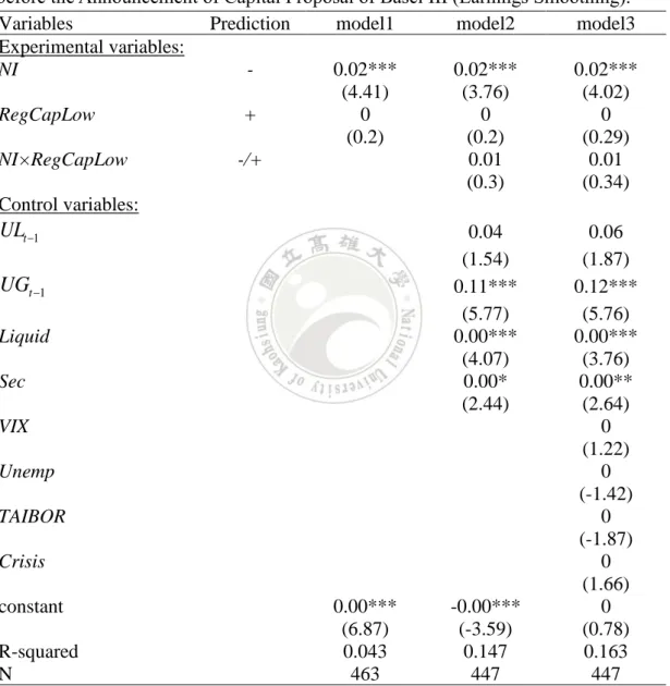
Table 7 shows regression summary statistic from equation (1). Net income before taxes and RGL (NI) is predicted to have a negative relationship to the realized gains and losses on AFS securities (RGL). Bank’s regulatory capital ratio before RGL and after taxes is equal one if it is in the lowest decile for the quarter, and zero otherwise (RegCapLow) is predicted to have a positive relationship to the RGL. The interaction of NI and RegCapLow is predicted to have negative or positive relationship to RGL.

The result of the first regression model shows net income before taxes and RGL (NI) is positively significant on realized gains and losses on AFS securities (RGL) at 1% level. The experiment result is not the same as the prediction. It should be noted that RegCapLow does not have significant effect on RGL. The second regression model adds the interaction of NI and RegCapLow. At the same time, the regression model also adds the other variables except for macroeconomic variables. The experiment result of

NI is also positively significant on RGL at 1% level. The experiment result of NI is also

not the same as the prediction. RegCapLow and NI×RegCapLow do not have significant effect on RGL. The third regression model adds the macroeconomics variables, such as implied volatility of options on the Taiwan Options Index (VIX), the number of people actively looking for a job as a percentage of the labor force in Taiwan (Unemp), Taipei Interbank Offered Rate (TAIBOR), and Financial crisis dummy variables (Crisis). The result of second regression model is similar to the first regression model, which NI is positively significant on RGL at 1% level.

The finding is not consistent with the prediction. When NI is positively significant on RGL, the banks tend to take big baths rather than realize securities gains and losses to smooth earnings. Table 7 also shows that the NI×RegCapLow coefficient is not significantly different from zero, which indicates that there is no interaction between the incentives to smooth earnings and manage regulatory capital or that the interaction

(37)

for positive and negative NI banks offset. Furthermore, the control variables such as

UG is positive significant on RGL, which indicates banks realize more gains when they

have more accumulated unrealized gains.

Table 7: Summary statistics from regressions of realized AFS securities gains and losses before the Announcement of Capital Proposal of Basel III (Earnings Smoothing).

Variables Prediction model1 model2 model3 Experimental variables: NI - 0.02*** 0.02*** 0.02*** (4.41) (3.76) (4.02) RegCapLow + 0 0 0 (0.2) (0.2) (0.29) NI× RegCapLow -/+ 0.01 0.01 (0.3) (0.34) Control variables: 1 t UL₋ 0.04 0.06 (1.54) (1.87) 1 t UG₋ 0.11*** 0.12*** (5.77) (5.76) Liquid 0.00*** 0.00*** (4.07) (3.76) Sec 0.00* 0.00** (2.44) (2.64) VIX 0 (1.22) Unemp 0 (-1.42) TAIBOR 0 (-1.87) Crisis 0 (1.66) constant 0.00*** -0.00*** 0 (6.87) (-3.59) (0.78) R-squared 0.043 0.147 0.163 N 463 447 447

(38)

4.3.2 After the Announcement of Capital Proposal of Basel III

Equation (1) also tests the Earnings Smoothing Hypothesis after the announcement of capital proposal of Basel III. The sample period is from year 2013 to 2017, which it does not have financial crisis. Table 8 shows regression summary statistic from equation (1). The prediction of NI, RegCapLow, and NI×RegCapLow is the same as the prediction in Table 7.

In contrast to the result of prediction, Table 8 shows the first regression model shows net income before taxes and RGL (NI) is positively significant on realized gains and losses on AFS securities (RGL) at 1% level. The second regression model also shows NI is positively significant on RGL at 1% level. The third regression model also reveals NI is positively significant on RGL at 1% level. When NI is positively significant on RGL, the banks tend to take big baths rather than realize securities gains and losses to smooth earnings.

The NI×RegCapLow coefficient is not significantly different from zero, which indicates that there is no interaction between the incentives to smooth earnings and manage regulatory capital or that the interaction for positive and negative NI banks offset. The control variables such as UL, UG, Liquid, and Sec have significant effect on RGL. UL and UG are positive significant on RGL, which indicates banks realize more losses (gains) when they have more accumulated unrealized losses (gains).

(39)

Table 8: Summary statistics from regressions of realized AFS securities gains and losses after the Announcement of Capital Proposal of Basel III (Earnings Smoothing).

Variables Prediction model1 model2 model3 Experimental variables: NI - 0.06*** 0.04* 0.04** (5.57) (2.46) (2.87) RegCapLow + 0 0 0 (0.47) (0.31) (0.33) NI× RegCapLow -/+ 0 0 (-0.01) 0 Control variables: 1 t UL₋ 0.17*** 0.16*** (4.74) (4.47) 1 t UG₋ 0.13*** 0.13*** (8.21) (8.2) Liquid 0.00*** 0.00*** (6.1) (6.11) Sec 0.00*** 0.00* (3.41) (2.1) VIX 0 (0.72) Unemp 0 (-0.79) TAIBOR 0 (-1.15) constant 0 -0.00*** 0 (0.66) (-7.24) (-0.34) R-squared 0.057 0.306 0.311 N 548 490 490

Note: ***, **, * indicate statistical significance at the 1%, 5%, and 10% level respectively.

4.4 Big baths for managing earnings

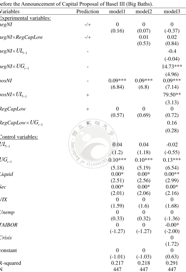
4.4.1 Before the Announcement of Capital Proposal of Basel III

Equation (2) tests the Big Baths Hypothesis before the announcement of capital proposal of Basel III. The hypothesis determines whether banks with negative earnings use realized AFS securities losses and gains to engage in big bath for managing earnings if their unrealized gains are insufficient to offset the negative earnings. Because the

(40)

financial crisis occurred in 2008 and 2009, the variable Crisis is also considered to equation on. The sample period is from year 2008 to 2012.

Table 9 shows regression summary statistic from equation (2). Net income before taxes and RGL (NI) is separated to positive and negative NI observations. The negative

NI (negNI) is predicted to have negative or positive relationship to RGL. The positive NI (posNI) is predicted to have negative relationship to RGL. Bank’s regulatory capital

ratio before RGL and after taxes is equal one if it is in the lowest decile for the quarter, and zero otherwise (RegCapLow) is predicted to have a positive relationship to the RGL. The interaction of negNI and RegCapLow is predicted to have negative or positive

relationship to RGL. The interaction of negNI and UL (UG) is predicted to have

negative relationship to the RGL. The interaction of posNI and UL is predicted to have relationship to the RGL. The interaction of RegCapLow and UG is predicted to have relationship to the RGL.

The results of three regression models of negNI coefficients is zero and it is not significantly different from zero. Table 9 also shows that the posNI coefficients are significantly positive in all three regression models, which indicates that banks with more positive earnings realize more gains or fewer losses on AFS securities. It indicates the banks take a big bath.

Compared to equation (1), equation (2) is attributable to distinguishing positive and negative NI banks, which shows more interaction between the variables to manage earnings and regulatory capital. The negNI×UG_t₋₁ is significantly positive at 1% level, which indicates that banks with more negative earnings realize fewer net gains on AFS securities when they have more accumulated unrealized gains. The posNI×ULt−1 is