國
立
交
通
大
學
財務金融研究所
碩
士
論
文
不 同 估 計 方 法 對 資 產 配 置 的 影 響
P o r t f o l i o A l l o c a t i o n w i t h D i f f e r e n t A p p r o a c h e s
研 究 生:陳岐穎
指導教授:周幼珍 博士
中 華 民 國 一百 年 六 月
i
不同估計方法對資產配置的影響
Portfolio Allocation with Different Approaches
研 究 生:陳岐穎 Student:Qi-Ying Chen
指導教授:周幼珍 博士 Advisor:Yow-Jen Jou
國 立 交 通 大 學
財 務 金 融 所
碩 士 論 文
A ThesisSubmitted to Graduate Institute of Finance College of Management
National Chiao Tung University in partial Fulfillment of the Requirements
for the Degree of Master
of
Science in Finance June 2011
Hsinchu, Taiwan, Republic of China
ii
不同估計方法對資產配置的影響
學生 : 陳岐穎 指導教授 : 周幼珍 博士
國立交通大學財務金融所 碩士班
中文摘要
一般傳統上常討論到使用 Markowitz 的均異最適化(mean-variance optimization) 的方式進行資產配置。由於 Markowitz 模型有估計誤差極大化的傾向,可發現報酬率些 微改變將造成重大影響,因此我們必須尋找較佳的方法估計報酬率以及變異數,以求得 較合理之投資權重。
Black and Litterman 以及其他學者運用不同的資訊,提出相對應的報酬率或變異 數的貝氏估計式,以改善 Markowitz 模型的缺點。本研究在 Black and Litterman 模型 上做了應用,本研究不僅估計報酬率同時也一起估計變異數。在根據這些不同的估計方 法,創造出最佳的資產配置,並且比較傳統 Markowitz 模型、Bootstrap 法及各種貝氏 估計法所得的投資組合 Sharpe ratio。
實證結果在我們的資料上發現在 Black and Litterman 模型與 Shrinkage 下,會得 到比較高的 Sharpe ratio。由於此兩種方法不僅對報酬率的估計上做了修正,也對變異 數方面做了估計,可以得到一個風險比較小的投資組合。表示此兩種方法在我們的資料 下,風險及報酬的表現優於其他兩種方法。
iii
Portfolio Allocation with Different Approaches
Student:Qi-Ying Chen Advisor:Yow-Jen Jou
Graduate Institute of Finance
National Chiao Tung University
ABSTRACT
This paper applies some popular asset allocation models, like Black-Litterman
model on an index fund. First, an overview is given of the foundations of
modern portfolio theory with the mean-variance model. Although the model
inspired a rich field of science and was used by many investors, it does have
some obvious flaws. Next, we discuss some improvements that could be made
over the mean-variance model. Finally, we compare the performance of the
bootstrap methodology, Black-Litterman model, Bayesian approach and
shrinkage methodology with the Sharpe ratio. The conclusion in our data can be
drawn that BL-model improves the mean-variance model and has a better
performance than other methods.
Keyword: Mean-Variance model, Asset Allocation, Black-Litterman model,
Bayesian approach
iv Contents 中文摘要 ... ii ABSTRACT ... iii Contents ... iv Table Contents ... vi Figure Contents ... vi 1、 Introduction ... 1 2、Literature Review ... 2
2.1 Introduction of Index fund ... 2
2.1.1 The advantages of Index Fund ... 3
2.2 Markowitz Mean-Variance Portfolio Selection Model... 3
2.2.1 Portfolio Selection Problem Formulations ... 4
2.3 The Black Litterman Model ... 5
3、 Methodology ... 8
3.1 Bootstrap Methodology ... 8
3.2 Black-Litterman Methodology ... 9
3.2.1 Computing the CAPM Equilibrium Excess Returns ... 11
3.2.2 Computing Via Reverse Optimization ... 11
3.2.3 Specifying the Views ... 13
3.2.4 Predicting of Covariance Matrix by GARCH Model... 14
3.2.5 The Black-Litterman Formula ... 15
3.3 Bayesian Approach ... 17
3.4 Shrinkage Methodology ... 18
4、Empirical Results ... 19
4.1 Data ... 19
4.2 Foreign Exchange Risk ... 20
4.3 Markowitz Method ... 20
4.4 Bootstrap Method ... 21
4.5 Black-Litterman Method ... 21
4.6 Bayesian Approach ... 22
v
4.8 Comparison of Markowitz Method and Other Approaches ... 23
4.8.1 Comparison of Portfolio Weights ... 23
4.8.2 Comparisons of Return, Risk and Sharpe Ratio ... 24
5、 Conclusion and Suggestions ... 25
5.1 Conclusion ... 25
5.2 Suggestions ... 25
6、 Reference ... 26
vi
Table Contents
Table 1: the parameter about Black-Litterman model ... 16
Table 2:Summary statistics for the country-specific returns ... 28
Table 3:Historical correlations of excess returns... 29
Table 4: Description of the parameters and data used in Markowitz method ... 30
Table 5: Summaries the allocations and resulting returns with Markowitz and Bootstrap ... 31
Table 6: Description of the parameters used in Black-Litterman method ... 32
Table 7:GARCH family results for estimate the investors‟ views ... 33
Table 8:Allocations with Black-Litterman model on three different confidence ... 34
Table 9:Description of the parameters used in the Bayesian approach ... 35
Table 10:Summaries the allocations and resulting returns of Bayesian approach ... 36
Table 11:Description of the Shrinkage mean with k=0.1798 ... 37
Table 12:Description of the Shrinkage covariance ... 38
Table 13:Summarizes the allocations and resulting return of all methods ... 39
Table 14:Compare return, risk and Sharpe ratio ... 40
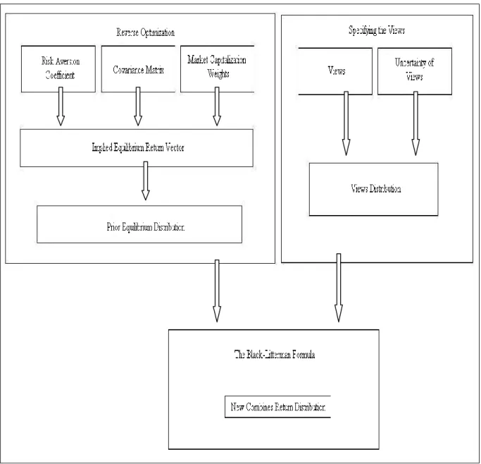
Figure Contents Figure 1 : The process of deriving the New Combined Return Vector ... 10
Figure 2:Mean distribution and convergence chart ... 35
1
1、 Introduction
Portfolio selection is concerned with selecting a portfolio of investments that will fulfill the investment objectives over the investment horizon. Although these objectives are different among investors, a positive and stable payoff on the investments is always desirable.
With innovating of the information network and economic globalization, International asset allocation gradually becomes a hot topic. There are some quantitative approaches to portfolio selection. The quantitative approach uses a mathematical model to make the final allocation of investments. The model evaluates the characteristics of investments and determines which ones should be added to the portfolio, then compute the optimal weights. In this research, we assumed assets are known in the portfolio and focus on the portfolio weights. Harry Markowitz is the founder of quantitatively making investment decisions. Key factor of asset allocation is to determine the portfolio return and risk. In his seminal paper (1952), he found out that when we gather the assets with the same returns into one portfolio, the risk of this portfolio would be lower than a single asset itself. Furthermore if the correlation between the assets including in the portfolio is lower, the portfolio risk would be more diversifiable in order to avoid the so-called “non-systematic risk". It requires two inputs:The expected (excess) return for each stock and the risk of each stock. Although the model inspired a rich field of science and was used by many investors, it does have some obvious flaws. For instance, the true parameters (the expected returns and risks) are unknown and have to be estimated from data. When investors impose no constraints, asset weights in the optimized portfolios almost always have large short positions in many assets; when constraints rule out short positions, the models often prescribe “corner” solutions with zero weights in many assets. Hence, it is difficult to implement the optimized mean-variance solution in practice. These unreasonable results come from two problems. First, expected returns are very difficult to estimate. Second, the optimal asset weights in standard asset allocation models are extremely sensitive to the expected return assumptions (Black-Litterman, 1991). The standard statistical method to estimate the covariance matrix of stock returns is to compute the sample covariance matrix. However, the sample covariance matrix contains a lot of estimation error. Feeding the sample covariance matrix to a mean-variance optimizer will result in “extreme “portfolio weights. Michaud (1989) calls this phenomenon “error-maximization”.
2
means of estimating expected returns to achieve better-behaved portfolio models. Actually the model of Black and Litterman differs from the Markowitz model only with respect to the estimation of expected return. The Black-Litterman model sets the idealized market equilibrium as a point of reference. The model then specifies a chosen number of market views in the form of expected returns and a level of confidence for each view. Combining the views and equilibrium returns, the Black-Litterman expected returns are obtained by Bayesian approach. The Black-Litterman expected returns are then optimized in a mean-variance way, creating a portfolio where investors have opinions about future expected returns.
An Index fund has been popular in these years, and how to allocate each index of the portfolio is also an important issue. We chose a Morgan Stanley emerging market index funds as the research object because recently the emerging market has been a hot top investment. Here, we apply the Bootstrap, Black-Litterman, Bayesian approach, Shrinkage methodology to constitute an index funds. Furthermore, we try to improve the Black-Litterman model by considering the shrinkage estimator of the covariance without using the historical sample covariance. The second section will do a quick review of the index fund, the Markowitz model, and literature about the Black-Litterman model. Subsequently, we arrive at the focus of our methodologies. The fourth section covers empirical results. Finally, we will discuss the differences between our methodologies by comparing the Sharpe ratio1.
2、Literature Review
This section reviews related literatures of this paper. First of all, we introduce the concept of index fund. Then we review the literatures related to the Black Litterman model.
2.1 Introduction of Index fund
Index funds are mutual funds that are intended to track the returns of a market index. A type of mutual fund with a portfolio constructed to match or track the components of a market index, such as the Standard & Poor‟s 500 index (S&P 500).
1 Sharpe ratio = p f p R R
3
2.1.1 The advantages of Index Fund
Investing in a collective investment scheme will increase diversity compared to a small investor directly holding a range of securities. Investing in an Index fund arrangement will achieve even greater diversification.
An investment manager may actively manage your investment with a view to selecting the best securities. An index fund manager will try to select the best performing index to invest in based upon the managers past performance and other factors. If the manager is skillful, this additional level of selection can provide greater stability and take on some of the risk relating to the decisions.
Going by the conception of “do not keep all eggs in one basket”, an index fund manager would invest in various securities which give investors benefits of diversification. By choosing a suitable Index fund, investors get a chance to invest across different classes of index within just one investment. Thus, it becomes very convenient for investing and monitoring.
2.2 Markowitz Mean-Variance Portfolio Selection Model
Mean-variance analysis presumes that return and risk (as measured by the portfolio variance) are all investors consider when making portfolio-selection decisions. Therefore, a rational investor would prefer a portfolio with a higher expected return for a given level of risk. An equivalent way to express the mean-variance principle is: a preferred portfolio is one that minimizes risk for a given expected return level. It is usually accepted that mean-variance analysis is grounded in either of two conditions: assets returns have a multivariate normal distribution or investor preferences are described by quadratic utilities. We start with some portfolio selection preliminaries. Suppose that there are N assets in which an investor may invest. Denote byRtthe excess returns on the N assets at time t,
' , , 1 ,..., ) ( t Nt t R R R , (1)
and assume that they have a multivariate normal distribution, ) , N( ) , ( Rt , (2)
with mean and covariance matrix given by the Nx1 vector and the NxN matrix, respectively. The portfolios weights are the proportions of wealth invested in each of the N assets and are given by the Nx1 vector (1,...N)'. A portfolio‟s return at time t is then
4 given by
N i t t i i p R R R 1 ' , (3)Its expected return and variance are defined, respectively, as
N i i i p 1 ' (4)where i is the expected return on asset i and
' 1 1 2 ) , cov( N i N j j i j i p R R (5)wherecov(Ri,Rj)is the covariance between the returns on assets i and j.
2.2.1 Portfolio Selection Problem Formulations
We assume that the investor‟s objective is to maximize his wealth at the end of his investment horizon, i.e. T+1, where T is the last period for which return data are available. We have added the subscripts T+1 in the notation for the expected returns and covariance to stress that these refer to attributes of unobserved asset returns. The mean-variance principle can be express through the following portfolio problems:
1 1 : . . 2 1 : max ' 1 ' 1 ' t s T T w (6)
where is the relative risk aversion parameter, a measure for the rate at which the investor is willing to accept additional risk for a one unit increase in expected return.
The composition of the investor‟s optimal portfolio (vector of optimal weights) is given by
1 1 1 ' 1 1 1 1 1 1 ' 1 1 ' 1 1 1 1 1 ' 1 1 1 1 1 1 1 * T T T T T T T T T T w (7)
More constraints are usually added to the optimization problems just given. For example, many institutional investors are not permitted to take short positions. In such cases, the portfolio weights are constrained to be positive, i 0,i1,...,N.
The classical mean-variance approach relies on the following two points. First, the unknown parameters are estimated from the sample of available data and the sample estimates are then treated as the true parameters. Second, it is implicitly assumed that the distribution of returns at the time of portfolio construction remains unchanged until the end of the portfolio holding
5
period. Usually, the sample estimates of and are computed as
T t t R T 1 1 ˆ ,
T t t t R R T 1 ' ) ˆ )( ˆ ( 1 1 ˆ (8)We re-express the vector of optimal portfolio positions in above as
ˆ ˆ 1 ˆ ˆ ˆ ˆ 1 1 ˆ 1 1 ˆ ˆ ˆ 1 1 * 1 ' 1 1 ' 1 ' 1 1 ' w (9)
Such an approach fails to recognize the fact that ˆ and ˆ may contain non-negligible amounts of estimation error. The resulting portfolio is quite often badly behaved, leveraging on assets with high estimated mean returns and low estimated risks, which are the ones most likely to contain high estimation errors. To deal with this, practitioners usually impose tight constraints on asset positions. However, this could lead to an optimal portfolio determined by the constraints instead of the optimization procedure. We consider the re-sampling, Black-Litterman, shrinkage methods to estimate the parameters.
2.3 The Black Litterman Model
This section provides a quick literature review of the Black-Litterman model. Black and Litterman initiated the first paper about Black-Litterman model in 1992, which provides a good discussion of the model along with the investor‟s view. However, they do not document all of their assumptions about the model. As a result, it is not easy to reproduce their results. They provide some of the key equations required to implement the Black-Litterman model, but they do not provide any equations for the posterior variance.
Bevan and Winkelmann (1998) used the Black-Litterman model for 3 years global fixed income investment portfolios with exchange rate hedging (from February 1995 to December 1997) and design an investment strategy. The empirical results show, 3-year performance is better than their target performance, and reached the level of risk management. According to the results of Goldman Sachs research department, Bevan and Winkelmann find out the market equilibrium return by setting a target Sharpe Ratio. Furthermore they offer guidance in setting the weight given to the view vector. After deriving an initial combined return (expected return) and the subsequent optimum portfolio weights, they calculate the anticipated Information Ratio of the new portfolio. They recommend a maximum anticipated Information Ratio of 2.0. If the Information Ratio is above 2.0, decrease the weight given to
6
the views. They also consider the market exposure and tracking error then compute the optimization portfolio weights subject to the given level of risk.
Litterman and Winkelmann (1996) proposed a new method to measure the market risk of the portfolio, called the market exposure. By this method one can clearly understand: the sensitivity of the market and investor‟s portfolio, i.e. the degree change of portfolio per unit of the market. General speaking, the market portfolio exposure is the regression coefficient of the portfolio on market. In practice, some bond fund managers use duration to measure the market risk but it need some assumptions.
He and Litterman (1999) says that the Black-Litterman asset allocation model have a very simple, intuitive property. The unconstrained optimal portfolio in the Black-Litterman model is the scaled market equilibrium portfolio (reflecting the uncertainty in the equilibrium expected returns) plus a weighted sum of portfolios representing the investor‟s views. The weight on a portfolio representing a view is positive when the view is more bullish than the one implied by the equilibrium and the other views. The weight increases as the investor becomes more bullish on the view, and the magnitude of the weight also increases as the investor becomes more confident about the view. However, when the capital budget and risk constraints are considered, the original intuitive property will not hold.
Lee (2000) and Christodoulakis (2002) clearly derived the expected excess returns of Black-Litterman model under the Bayesian approach also they say lack-Litterman model has some other meaning. First, even if the investors have no view for a specific individual asset, but the weight of specific individual asset still change from their original market capitalization weights due to some correlation between all assets in the portfolio. That is to say when the investors have views of other assets, implies they still have some view for that specific individual asset. Second, the Black-Litterman model overcomes the most-often cited weaknesses of mean-variance optimization (unintuitive, highly concentrated portfolios, input-sensitivity, and estimation error-maximization) by change the “confidence” in views. Ldzorek (2002) provided detail of how to estimate the parameters in model. According to the assumptions of CAPM, one can use the market capitalization weight, historical covariance matrix of return and the risk aversion of investors to compute the equilibrium excess return. The equilibrium excess return conditional on the investor‟s view is distributed with a covariance structure proportional to the historical covariance matrix of return. The scalar is a known quantity to the investor that scales the historical covariance matrix of return. Black and
7
Litterman (1992) and Lee (2000) say that the scalar would be close to 0; but some scholars2 think that would be close to 1. Fortunately, Ldzorek (2002) proposed a formula to solve this problem, the value of scalar depends on the investors‟ confidence level of views.
According to Litterman (2003) the uncertainty of the investor view means the error terms of the investor view are also a common question without a “universal answers”. Regarding to the error terms of investor view, Herold (2003) says that the major difficulty of the Black-Litterman model is that it forces the user to specify a probability density function for each view, which makes the Black-Litterman model only suitable for quantitative managers. Idzorek (2005) provides a new method for incorporating user-specified confidence levels in each view to determine value of the error terms of investor view, making the model more useful for all individual investor not only for specific quantitative managers.
Mankert (2006) analyzes the Black-Litterman model using both mathematical and behavioral finance approach. Mankert firstly makes use of sampling theoretical approach to generate a new interpretation of the model and gives an interpretable formula for the mystical parameter (scale of the historical covariance matrix of return). Secondly, she draws implications from research results within behavioral finance. One of the most interesting features of the Black-Litterman model is that the benchmark portfolio, against which the performance of the portfolio manager is evaluated, functions as the point of reference. According to behavioral finance, the actual utility function of the investor is reference-based and investors estimate losses and gains in relation to this benchmark. Implications drawn from research results within behavioral finance explain why the portfolio output given by the Black-Litterman model appears more intuitive to fund managers than portfolios generated by the Markowitz model. Another feature of the Black-Litterman model she proposes is that the user assigns levels of confidence to each asset view in the form of confidence intervals.
Liang (2002) studies the out-of-sample performance of the Black-Litterman model on international asset allocation. He used the short-run momentum to estimate the invertors‟ views.
Beach and Orlov (2006) provide an application of the Black-Litterman (1991, 1992) methodology to portfolio management in a global setting. They found an econometric model that accurately describes the dynamics of the excess returns on international portfolios and the dynamics of the returns volatility. They consider about asset returns are characterized by several stylized facts: volatility clustering, excess kurtosis, asymmetry, autocorrelation in risk,
2
8
time-varying volatility. They combine the exponential GARCH (Nelson, 1991) and GARCH-in-Mean (Engle, Lilien and Robins, 1987) models to take into account of these characteristics of financial data. They use GARCH-derived views as an input into the Black-Litterman model, since there is no model that effectively describes an investor views. After that, they use four different “confidence (scale of the historical covariance matrix of return)”-based Black-Litterman allocation series to investigate the confidence effect. They allow an investor to determine if the portfolio risk is higher than acceptable; the investor can alter the confidence parameter, until a risk-appropriate allocation is generated. Finally, they found out the risk-tailored portfolio produced the highest returns of the portfolios considered, with lower risk than the original Black-Litterman result.
3、 Methodology
This section we will illustrate our approaches to the portfolio allocation. First of all, we introduce the bootstrap approach which is easy to understand and widely used. Second, we will discuss about the Black-Litterman model in detail. Finally, we introduce the Bayesian and shrinkage approach.
3.1 Bootstrap Methodology
Re-sampling methods are widely used in modern statistics. They use Monte Carlo Simulation to compute many statistically similar alternatives to enhance the information in a data set for analysis and estimation. In this section, we will describe the re-sampling methodology to improve the shortcoming of mean-variance theorem. In this approach, we use the historical data to compute the sample covariance matrix in place of the unknown true covariance matrix. We use bootstrap to avoid solely relying on the sample mean computed from past returns. The algorithm is as follows.
Step 1 :Resample from the past returns to create a bootstrap sequence of returns, the number of the data point in bootstrap sequence should be the same as in the original sample.
Step 2 :Compute the sample mean and sample covariance matrix from the bootstrap data call it X and S*.
9
optimal vector of weightsw . *
Step 4 :Repeat Step1~3 K times and average over the K weight vectorsw to obtain the final *
vector of portfolio weights.
There are two possibilities for the re-sampling in Step 1. One can resample from a parametric estimate of the underlying distribution, such as the normal distribution whose mean is the sample mean of the past returns and covariance matrix is the sample covariance matrix of the past returns. Alternatively, one can resample from the observed data with replacement. The two approaches yield very similar results in practice; here we use the second method to resample the data. Besides the bootstrap methodology, we examine the Bayesian approach to dealing with estimation risk in portfolio optimization, briefly discussing Black-Litterman model and shrinkage estimators.
3.2 Black-Litterman Methodology
The Black-Litterman model makes two significant contributions to the problem of asset allocation. First, it provides an intuitive prior, the CAPM equilibrium market portfolio, as a starting point for the application of Bayesian techniques to estimate returns. The idea that one could use „reverse optimization‟ to generate a stable distribution of returns from the CAPM market portfolio as a starting point is a significant improvement to the process of return estimation.
Second, it provides a clear way to specify investors‟ views and to blend the investors‟ views with prior information using Bayesian techniques. This process estimates expected return and covariance which can be used as input to an optimizer. Before their paper, nothing similar had been published. The mixing process had been studied, but nobody had applied it to the problem of estimating returns. No research linked the process of specifying views to the blending of the prior and the investors‟ views. The Black-Litterman model provides a quantitative framework for specifying the investors‟ views, and a clear way to combine those investor‟s views with an intuitive prior to arrive at a new combined distribution. This process is presented as Figure 1 and it can be divided into three parts: Reverse optimization, specifying the views, and the Black-Litterman formula. Besides, we consider use shrinkage techniques to shrunk the sample covariance matrix, modify the drawbacks that Black-Litterman model only consider the historical sample covariance matrix.
10
11
3.2.1 Computing the CAPM Equilibrium Excess Returns
The process of computing the CAPM equilibrium excess returns is straight forward. These returns will provide the prior distribution for the Black-Litterman model.
CAPM is based on the concept that there is a linear relationship between risk and return. Further, it requires returns to be normally distribution. This model is of the form
m f r r r E( ) (10) where f
r The risk free rate
m
r The excess return of the market portfolio
A regression coefficient computed as
m p
The residual or asset specific excess return
Under the CAPM theory the investor is reward for the systemic risk measured by, but is not rewarded for taking non-systemic risk associated with . This is because within a diversified portfolio the total should tend to 0 in the limit.
The CAPM theory states that all investors should hold the market portfolio as their risky asset. They may hold arbitrary fractions of their wealth in the risky asset and the remainder in the risk-free asset depending on their degrees of risk aversion. The market portfolio is on the efficient frontier, and has the maximum Sharpe Ratio of any portfolio on the efficient frontier. Because all investors hold only this portfolio of risky assets, at equilibrium the market capitalizations of the various assets will determine their weights in the market portfolio. Now we start with the „reverse optimization‟ for compute the equilibrium excess returns.
3.2.2 Computing Via Reverse Optimization
This section, we derive the equations for „reverse optimization‟ starting from the quadratic utility function. Throughout this paper, K is used to represent the number of views and N is used to represent the number of funds in the portfolio.
w w w U T ) T 2 ( (11) where
U : The investor‟s utility; the objective function during portfolio optimization w : The vector of weights invested in each asset (N x 1 column vector)
12
: The vector of equilibrium excess returns for each asset (N x 1 column vector)
: The risk aversion parameter of the market
: The covariance matrix of excess returns (N x N matrix)
We will constrain the problem by asserting that the covariance matrix of the return is known3. The investor‟s utility U is a concave function, so it will have a single global maximum. If we maximize the utility with no constraints there is a closed form solution. We find the exact solution by taking the first derivative of (11) with respect to the weights and setting it to 0. Solving this for yields (12)
mkt w (12) where mkt
w : The market capitalization weight of the assets (N x 1 column vector)
The Black-Litterman model uses „equilibrium‟ returns as a neutral starting point. Equilibrium returns are the set of returns that clear the market. The equilibrium returns are derived using a reverse optimization method in which the vector of implied excess equilibrium returns is extracted from known information using formula (12).
In order to use formula (12) we need to have a value for, the risk aversion coefficient of the market. We can find by multiplying both sides of (12) by wmktT and replacing vector
terms with scalar terms.
2 ) ( m f m r r E (13) whereE(r) : the total return on the market portfolio (E(r)rf) f
r : the risk free rate
2
m
: the variance of the market portfolio (m2 wmktT wmkt)
As part of our analysis we must arrive at the terms on the right hand side of formula (13); E(r),rf andm2 in order to calculate a value for. When we have a value for , then we plug w, and into formula (12) and generate the equilibrium asset returns. Formula (12) is the closed form solution to the reverse optimization problem for computing asset returns given an optimal mean-variance portfolio in the absence of constraints. Furthermore if we feed, and back into the formula (12), we also can solve for the weights (w). If we use
13
historical excess returns rather than equilibrium excess returns, the results will be very sensitive to changes in .with the Black-Litterman model, the weight vector is less sensitive to the reverse optimized vector. This stability of the optimization process is one of the strengths of the Black-Litterman model.
3.2.3 Specifying the Views
We will describe the process of specifying the investors‟ views of estimated returns. We define the combination of the investors‟ views as the prior distribution. First, we will require each view to be unique and uncorrelated with the other views. This will give the prior distribution the property that the covariance matrix will be diagonal, with all off diagonal entries equal to 0. We constrain the problem this way in order to simplify the problem and improve the stability of the results. Second, we will require views to be fully invested; either the sum of weights in a view is zero (relative view) or is one (an absolute view).
We will represent the investors‟ K views on N assets used the following matrices.
1. P is a K x N matrix of the asset weights within each view, for a relative view the sum of weights will be 0, for an absolute view the sum of the weights will be 1.
N K K N p p p p P , 1 , , 1 1 , 1 (14)
Different authors compute the various weights within the view differently; Idzorek uses a capitalization weighed scheme, whereas others use an equal weighted scheme. Here we use the capitalization weighed scheme.
2. Q is a K x 1 matrix of the returns for each view.
3. Ω is a K x K matrix of the covariance of the views. Ω is diagonal as the views are required to be independent. 1 is known as the confidence in the investors‟ views. The i-th diagonal element of Ω is represented asi.
As an example of how these matrices be populated we have 3 assets and two views. First, a relative view in which the investor believes that asset 1 will outperform asset 2 by 4% with confidence1. Second, an absolute view in which the investor believes that asset 3 will return 3% with confidence2. These views are specified as follows:
1 0 0 0 1 1 P ; 3 4 Q ; 2 1 0 0
14
space as:
PE(r) ~ N (Q, Ω) (15)
There are four main ways to calculate Ω. First, we actually compute the variance of the view. Second, we can just assume that the variance of the view will be proportional to the variance of the assets, just as the variance of the sampling distribution is. He and Litterman (1999) use this method, and we can use the variance of the view computed from the sampling distribution: ) )P (P( diag T (16)
Idzorek (2004) introduces the third method. He allows the specification of the view confidence in terms of the percentage move of the weights from no views to total certainty in the view.
Beach and Orlov (2006) introduce the final method. They consider about asset returns are characterized by several stylized facts: volatility clustering, excess kurtosis, asymmetry, autocorrelation in risk, time-varying volatility. They use GARCH-derived views as an input into the Black-Litterman model. Here, we use GARCH-derived views as proxies for investor views in the Black-Litterman model. It is useful for expository purposes, since there is no model that effectively describes an investor‟s views.
3.2.4 Predicting of Covariance Matrix by GARCH Model
The GARCH model offers a more parsimonious model that reduces the computational burden. It uses past variances and past variance forecasts to forecast future variances. The model is quite successful in predicting conditional variances. GARCH models allow not only forecasting conditional means of asset returns, but also conditional variances. We combine the ARCH-in-Mean model to relate the expected return on assets to the expected risk, and the Exponential GARCH model to allow for asymmetric shocks to volatility.
GARCH (p, q)
In general, a GARCH model can be represented by two equations - one for the conditional mean and the other for the conditional variance:
) , 0 ( ~ , t 2 ' t t t t x N y (17)
q j j t j p i i t i t 1 2 1 2 2 (18)15
where:
t
y : The dependent variable (i.e. excess return)
t
x : Vector of exogenous variables
, and are the coefficients to be estimated. The one-period ahead forecast variance
2
t
(conditional variance) depends on the mean (), news about volatility from the previous period (t2i, the ARCH term), and last period‟s forecast variance (
2
j t
, the GARCH term).
GARCH (p, q) refers to the presence of q-order GARCH term and p-order ARCH term.
EGARCH-M (p, q)
Exponential GARCH models are able to account for asymmetric shocks to volatility. ARCH-in-Mean models introduce the conditional variance into the mean equation.
ˆ2 ' t t t t x y (19)
q i t i i t i i t i p j j t j t 1 1 2 2 ˆ log (20)This EGARCH-M (p, q) model is used to estimate expected returns (Q) and conditional variance (). The log implies that the leverage effect is exponential, thus forecasts of the conditional variance are guaranteed to be nonnegative. The EGARCH model is able to capture the empirical regularity that a negative shock leads to a relatively higher conditional variance than a positive shock of the same magnitude.
3.2.5 The Black-Litterman Formula
Applying Bayes theory to the problem of blending the sampling and prior distributions, we can create a new posterior distribution of the asset returns. We can derive the equation4 for the posterior distribution of asset returns.
) P) P ) (( , P] P ) Q][( P ) ([( N ) (R -1 T-1 -1 T-1 -1 -1 T-1 -1 E (21) where:
E(R) : the new combined return vector (K x 1)
: a scalar
: the covariance matrix of excess returns (N x N)
16
P : a matrix that identifies the assets involved in the views (K x N)
: a diagonal covariance matrix of error terms from the expressed views (K x K)
: the implied equilibrium return vector Q : the view vector
We can represent the same formula for the mean returns in an alternative way:
-1 -1 T -1 -1 T -1 P] P ) Q][( P ) [( ) (R E (22)
Eq. (22) is the new combined return vector, and with all of the inputs and then entered into Eq. (22) new combined return vector is derived. The new recommended weights (w ) can be *
calculated by solving Eq. (9). The table 1 will show the detail about the Black-Litterman model‟s parameters.
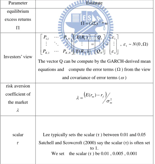
Table 1: the parameter about Black-Litterman model
Parameter Estimate equilibrium excess returns ( ) *w -1 Investors‟ view ) , 0 ( ~ , ) ( ) ( t 1 1 1 , 1 , , 1 1 , 1 N Q Q R E R E P P P P n N N N K K N
The vector Q can be compute by the GARCH-derived mean equations and compute the error terms () from the view
and covariance of error terms () risk aversion coefficient of the market
2 ) ( m f m r r E scalar Lee typically sets the scalar (τ ) between 0.01 and 0.05 Satchell and Scowcroft (2000) say the scalar (τ) is often set
to 1.
17
3.3 Bayesian Approach
The classical approach to asset allocation is a two-step process: first the market distribution is estimated, the optimization is performed. But the classical „optimal‟ allocation is not truly optimal; the optimization process is extremely sensitive to the input parameters. Bayesian theory provides a way to limit the sensitivity of the final allocation to the input parameters by shrinking the estimate of the parameters. We will introduce the Bayesian approach under the standard normal-inverse-Wishart conjugate assumption for the market. Suppose now that the investor has informative beliefs about the mean vector and the covariance matrix of excess returns. We consider the case of conjugate priors the conjugate prior for the unknown covariance matrix of the normal distribution is the inverted Wishart distribution, while the conjugate prior for the mean vector of the normal distribution (conditional on ) is multivariate normal. We make the following assumptions: first, the market consists of equity-like securities for which the returns are independently and identically distributed across time; second, the estimation interval is the same as the investment horizon; third, the returns are normally distributed:
) , ( ~ , N Rt (23)
Then, we model the investor‟s prior experience as a normal-inverse-Wishart distribution:
k 1 , ~N Q , ~IW(,m) (24)
Where (Q,) represent the investor‟s experience on the parameters, whereas (k,m) represent the respective confidence. The prior parameter k determines the strength of the confidence the investor places on the value Q. When k=0, the variance of is infinite and its prior distribution becomes completely flat-the investors has no knowledge or intuition about the mean and let it vary uniformly from to. It is important to notice that and
is no longer independent in the prior (23). This prior dependence might not be unreasonable if the investor believes that higher risk could entail greater expected returns. It is possible to compute the posterior distribution of and under the above hypotheses. First, the information from the market is summarized in the sample mean and the sample covariance of the past realizations of the returns:
T t t t T t t r r r 1 ' 1 ) )( ( 1 -T 1 , T 1 (25)18
The posterior distribution of next-period‟s excess returns can be shown to be multivariate Student‟s t. The central limit theorem5
asserts that for large sample size, the distribution is approximately normal distribution. The mean of the predicted excess returns and their covariance matrix can be shown to be:
) ~ k N 1 , kQ) ˆ (N k N 1 N( ~ ~ , ˆ ~ (26) ) m N , ) ˆ )( ˆ ( ( W ~ ˆ , ˆ ~ -1 ' Q Q K N NK NS (27) where t
r : The excess returns on the N assets at time t N : number of asset
The predictive mean in (26) is a weighted average of the prior mean Q and the sample mean
ˆ -the sample mean is shrunk toward the prior mean. The stronger the investor‟s belief in the prior mean is (the higher
k N
k
is), the larger the degree to which the prior mean
influences the predictive mean (the degree of shrinkage). When the investor has 100% confidence in the prior mean, the predictive mean is equal to the prior mean, ~ =Q and the observed data in fact become irrelevant to the determination of the predictive mean.
3.4 Shrinkage Methodology
A shrinkage estimator is a weighted average of the sample estimator and another estimator. Stein (1956) showed that shrinkage estimators for the mean, although not unbiased, possess more desirable qualities than the sample mean. The so-called James-Stein6 estimator of the mean has the general form:
1-k ˆ 0JS k (28)
where the weight k, called the shrinkage intensity, is given by
0 ' 0 ˆ -ˆ T 2 -N , 1 min k (29)It is interesting to notice that any point 0 can serve as the shrinkage target. The resulting
5 CLT: The distribution of sample means from smaller samples is better represented by Student's t-distribution, which converges to the normalized Gaussian distribution as the sample size increases
6
19
shrinkage estimator is still better than the sample mean. However, the closer 0 is to the true mean, the greater the gains are from using JS in place of ˆ . Therefore, 0 is often chosen to be the prediction of a model for the unknown parameter .
Shrinkage estimator for the covariance matrix has also been developed. For example, Ledoit and Wolf7 (2003) propose that the covariance matrix from the single-factor model of Sharpe (1963) (the single factor is the market) be used as a shrinkage target:
1- S LW (30) T k , 1 min , 0 max (31)where S is the sample covariance matrix and is the covariance matrix estimated from the single-factor model. The shrinkage intensity can be shown to be inversely proportional to number of return observations. The constant of proportionality k is dependent on the correlation between the estimation error in S and the misspecification error in .
4、Empirical Results
4.1 Data
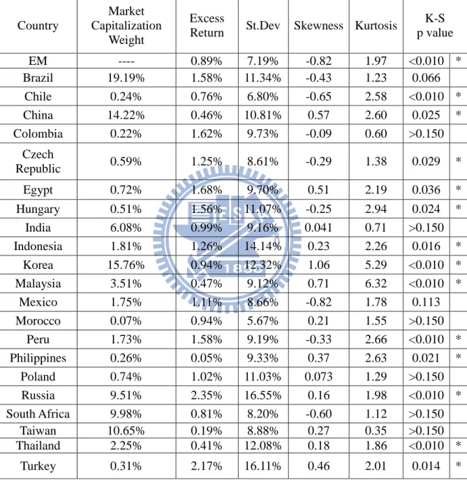
We use 15 years of monthly data from January 1995 to September 2010 (189 months). The equity returns are from the Morgan Stanley Capital International (MSCI) Emerging Markets Index with gross dividends reinvested. We use one-month Eurodollar rate as a risk-free return8. The MSCI Emerging Markets Index is a free float-adjusted market capitalization index that is designed to measure equity market performance of emerging markets. The MSCI Emerging Markets Index consists of the following 21 emerging market country indices: Brazil, Chile, China, Colombia, Czech Republic, Egypt, Hungary, India, Indonesia, Korea, Malaysia, Mexico, Morocco, Peru, Philippines, Poland, Russia, South Africa, Taiwan, Thailand, and Turkey. Table 2 presents summary statistics for the country-specific returns. Fourteen countries reject normality based on Kolmogorov-Smirnov statistic. Positive or negative
7 Detail describe from Ledoit and Wolf (2003) , Honey, I Shrunk the Sample Covariance Matrix 8 Source form Federal Reserve Board of Governors system with one month Eurodollar rate
20
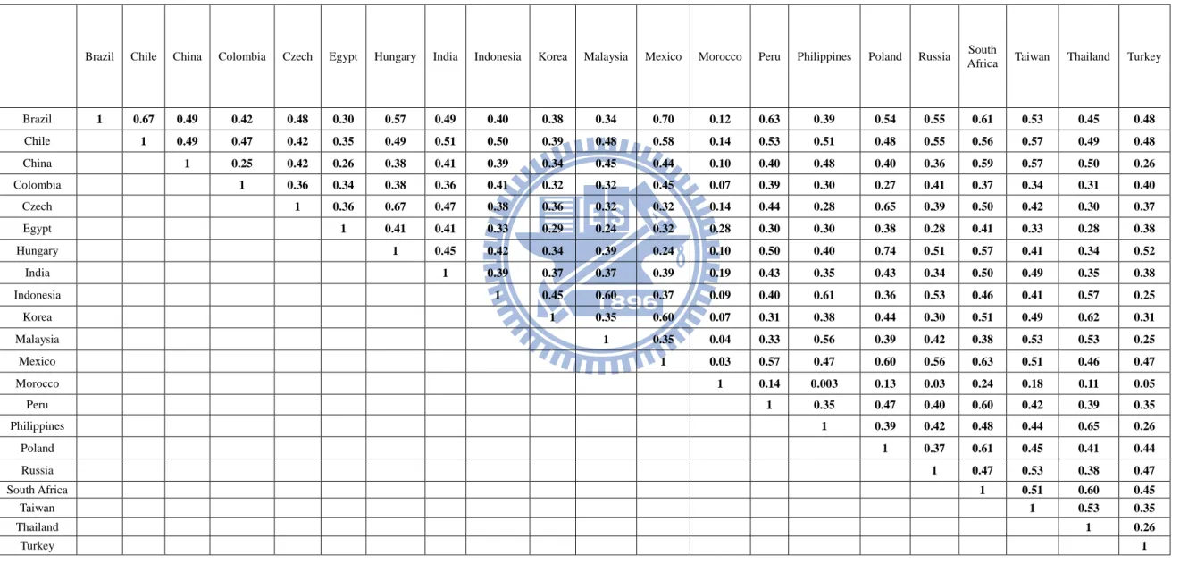
skewness is observed for many markets. Excess kurtosis is indicated for most of the return series. The correlations are in Table 3. All results in the paper have a U.S. dollar perspective.
4.2 Foreign Exchange Risk
The hedging of foreign exchange risk in an international portfolio is a significant decision that should be grounded in several practical and theoretical considerations. If purchasing power parity holds (and investors globally hold the same consumption basket), then the hedging of foreign currency risk would not be necessary, because the currency returns would exactly reflect inflation differences around the globe. Since purchasing power parity is known to not hold, hedging currency risk may be optimal. In Black and Litterman (1992), an 80% hedge ratio is applied, and the benefits of hedged are sizeable in a bond-only portfolio, at a 0.57% return advantage to the hedged portfolio, given a fixed risk level. For the equity-only portfolio, the return advantage for the hedge portfolio is only 0.08%, potentially insufficient to justify the cost in time and transaction costs.
Many individual investors and small portfolio shops combine the currency and equity allocation decisions, with no attempt to hedge the currency exposure. Possibly, they assume that currency fluctuations are random or mean-revert in a manner that makes the currency allocation irrelevant over an extended timeframe. Alternatively, an investor may believe that the combined allocation to equities and currencies can be managed more effectively than by making separate decisions. We have chosen not to hedge the foreign currency risk. This approach allows a focus on other salient components of the international asset allocation decision.
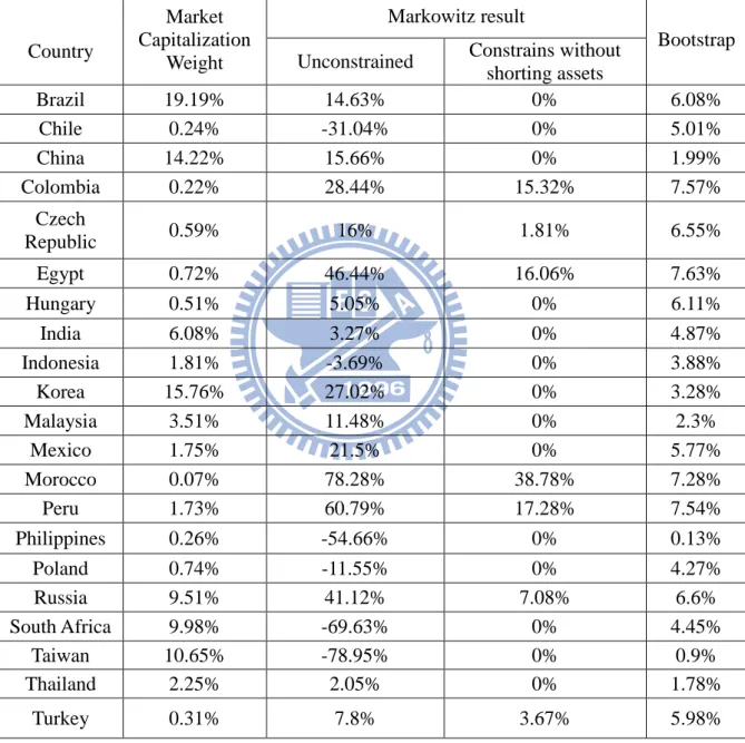
4.3 Markowitz Method
The Markowitz approach often assumes that excess returns will equal their historical averages. A description of the parameters and the data used are given in Table 4. The problem with this approach is that historical means are very poor forecasts of future returns. Table 5 illustrates when we use these historical excess returns as our expected excess return assumptions, with and without shorting constraints. We may make a number of points about these “optimal” portfolios. First, they illustrate what we mean by “unreasonable” when we claim that standard mean-variance optimization models often generate unreasonable portfolios. The portfolio that does not constrain against shorting has many large long and short positions with no obvious
21
relationship to the expected excess return assumptions. When we constrain shorting we have positive weights in six countries. These portfolios are typical of those that the standard model generates. Next part we will apply a variant of the resample efficiency of Michaud (1998).
4.4 Bootstrap Method
We resample from the past returns to create a bootstrap sequence returns then compute the sample mean and sample covariance matrix. Solve the quadratic optimization weights and repeat 10,000 times to obtain the final vector of portfolio weights. Results are also presented in the Table 5. It seems more reasonable with Markowitz approach results.
But Most of the time investors do have views- feelings that some assets are overvalued or undervalued at current market prices. An asset allocation model should help them to leverage those views to their greatest advantage. The basic problem that confronts investors trying to use quantitative asset allocation models is how to translate their views into a complete set of expected excess returns on assets that can be used as a basis for portfolio optimization. As above says, the problem is that optimal portfolio weights from a mean-variance model are incredibly sensitive to minor changes in expected excess returns. Next section we will present a GARCH model and Black-Litterman methodology of combining equilibrium weights with investor‟s subjective views.
4.5 Black-Litterman Method
The fundamental idea behind the Black-Litterman method is that the equilibrium that exists in the financial markets, represented by the existing capitalization weights, serves as the basis for establishing an optimal allocation. These market capitalization weights are used to establish implied equilibrium expected returns. The views held by the investor regarding expected returns are an additional input to the asset allocation decision. In our research presented in this paper, the GARCH families are used to provide the investor views and confidence measures for those views. The investment weights from the Black-Litterman method are then established by reverse optimization utilizing the blended return vector and the covariance matrix of historical returnsWi 1E(R)
. The proportional weights are
22
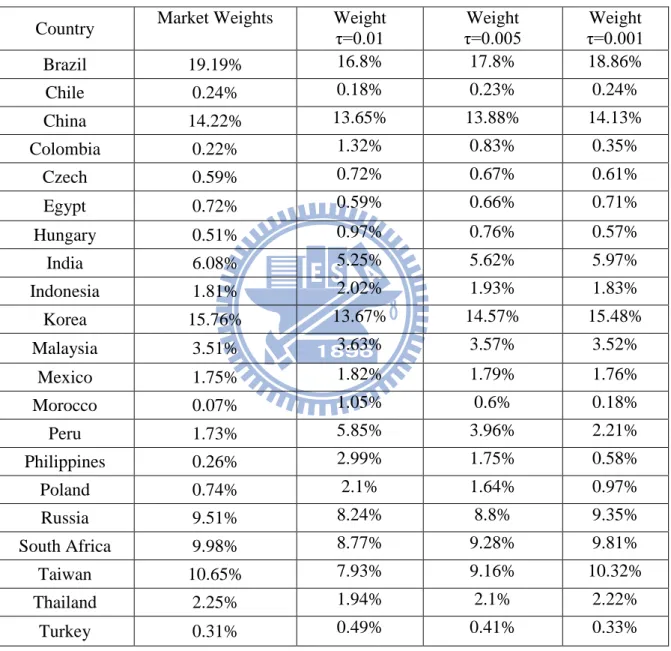
n i i i i W W w 1A description of the parameters and the data used in this paper are given in Table 6. The matrix is commonly referenced as reflecting the “confidence” in the views. Here we utilize one-period forward estimates of the variance from the EGARCH-M models (one estimate for each country, for each period) to provide the measure of confidence for each view. Table 7 present the EGARCH-M result for estimate the investors‟ views and Table 8 summarizes the allocations and resulting returns of portfolios using market allocations and three different „confidence‟ based Black-Litterman allocation series. As the τ measure of the confidence in the “Black-Litterman implied returns” is decreased, the weighting on the market weights is given more importance.
4.6 Bayesian Approach
We continue with our illustration based on the monthly excess returns of the MSCI country indexes. Solve the quadratic optimization weights and repeat 10,000 times to obtain the final vector of portfolio weights. We choose the hyper parameters in (25) as follows:
Q : We use GARCH model to estimate the Q. The reason for specifying Q is that we think
investors may have some informative beliefs about the mean vector of excess returns.
k : We set k equal to 188. k often takes on the interpretation of the size of a hypothetical sample drawn from the prior distribution: the larger the sample size, the greater our confidence in the prior parameter, Q.
Ω : The diagonal covariance matrix we use GARCH model to estimate the Ω .
m : is equal to 22. We choose a low value for the degrees of freedom to make the prior for
non-informative and reflect our uncertainty about Ω . The mean of the inverse Wishart random variable exists if m >N+1.
A description of the parameters and the data used in this paper are given in Table 9.
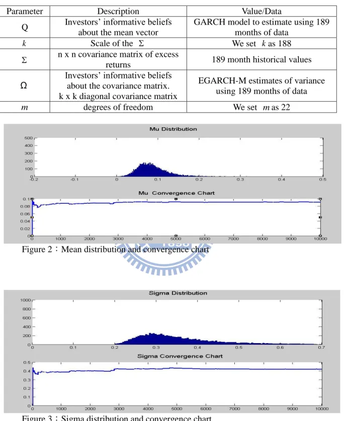
Table 10 summarizes the allocations and resulting returns of portfolios. It seems more reasonable with Markowitz approach results. Figure 2 present the mean distribution and convergence chart. Figure 3 present the covariance distribution and convergence chart.
23
4.7 Shrinkage Method
We now illustrate our last method using the shrinkage estimator to construct a portfolio based on our data. We first construct raw forecasts of the expected excess returns by shrinking the sample mean toward the shrinkage target. The historical average returns contain important information on future expected returns and should not be almost ignored. Here, we use GARCH model that accurately describes the dynamics of the excess returns and the dynamics of the returns volatility as our shrinkage target. Then, we construct a shrinkage estimator by using linear combination of the sample mean and our shrinkage target with shrinkage intensity. Table 11 present the results about the shrinkage mean.
In a second step, we proceed with the shrinkage estimators for the covariance matrix. We include the sample covariance matrix, the shrinkage estimator of Ledoit and Wolf9 (2003). It is to take a weighted average of the sample covariance matrix with Sharpe‟s (1963) single-index model estimator. Table 12 presents the results about the shrinkage covariance.
4.8 Comparison of Markowitz Method and Other Approaches
We want to see the difference of the index fund allocation with traditional Markowitz‟ method10 and our others approach. In the first part, we compare the allocations with different approaches. The second part demonstrates the comparison with Sharpe ratio of our different approaches.
4.8.1 Comparison of Portfolio Weights
Table 13 summarizes the allocations and resulting returns of our all methods. One can found out that besides the Markowitz method all methods get relatively balanced weights than the traditional Markowitz method with sample estimates.
As we discussed in the Section 2.2.1, there are many problems when using Markowitz‟ method to achieve optimal weights. Not surprisingly, weights with Markowitz‟ method based on historical return produce an extreme portfolio. Based on historical returns, the Markowitz model recommends the weights of 78.82%, 60.79%, and 46.44% on Morocco, Peru and Egypt, respectively, but recommends -78.95%, -69.63%, and -54.66% on the Taiwan, South Africa
9 Ledoit and Wolf suggest the single-factor model of Sharpe (1963) as the shrinkage target.
10 Markowitz‟ method has been discussed and improved. The Black-Litterman and other approaches can be regarded as an improved Markowitz‟ method as well. Markowitz‟ method represents the traditional optimization based on the historical return vector
24
and Philippines, respectively without constrained short limit. Once the short limits are imposed, the portfolio recommends 0% on many countries. The extreme result with Markowitz model may prevent investors from using the model.
Compared with the Markowitz model, the recommend weights with other approaches are not only reasonable but also more stable. For instance, the Black-Litterman approach recommends the 7.93%, 9.15% and 10.32% on Taiwan with different τ rather than 0% weight or large short, respectively. We now interest in which one approach would perform better, we consider comparing the return, risk, and Sharpe ratio. The results are present in Table 13.
4.8.2 Comparisons of Return, Risk and Sharpe Ratio
To make the baseline of our comparison, we first hold the investors only consider the return. The comparisons are presented in the Table 13. If investors only consider the absolute return we can found out the Bayesian approach generate the highest return and the second highest is Bootstrap than others. If investors care about the portfolio risk the Shrinkage approach prove the smallest standard deviation and the second smallest is Black-Litterman approach. In practice, when an investor choose which portfolios worth to invest they should not only consider the returns but also their risk. We choose the Sharpe ratio which is a measure of the excess return per unit of risk in investment assets. The Sharpe ratio has as its principal advantage that it is directly computable from any observed series of returns. As in Table 13 shown, the Black-litterman approach prove the highest Sharpe ratio and Shrinkage approach prove second highest than others.
Investors care about the profitability more than the stability of the portfolio. The Black-Litterman model may not result in a high absolute return in our research but it proves the high profitability with the highest Sharpe ratio. The attractiveness of the Black-Litterman is its combination of the investment strategies with quantitative methods.
25
5、 Conclusion and Suggestions
5.1 Conclusion
Mean-variance optimization has since its origination been the most popular method for asset allocations. The popularity could be due to the understandable premise on which it sorts assets. However, in practice, the mean-variance-portfolios are often generating unseasonable results and do not reflect the views of the investor. In order to cope with these problems, investors often constrain the mean-variance model in such way that the possible portfolios lie in a bandwidth they are comfortable with. Black and Litterman (1992) set out to alleviate these problems by making a model that would result in intuitively attractive portfolios and a model that could be used by investors.
The purpose of this study is to apply the popular asset allocation models such like Black-Litterman, Bootstrap, traditional Bayesian, Shrinkage methods for index finds. We carry out Sharpe ratio to compare the methods. We find the Black-Litterman model can produce the highest profitability than others in our case.
5.2 Suggestions
This study we do our best effort in relevant literature review and comparison of different models, but there are still many imperfections have to improvement. First, we only have sample period from January 1995 to September 2010 monthly data (189 data for each asset) without to do a long-term study for the portfolio. Second, we assume the parameter of Black-Litterman τ is known to construct a portfolio without estimate the unknown parameter of τ. Finally, we only focus on one period forecast, like T+1 without do multiple predictions. If future researcher can improve those imperfections, it will make the model more flexible and useful.
26
6、 Reference
[1] Anderson, T. W. (1984), An Introduction to Multivariate Statistical Analysis (2nd ed.), John Wiley & Sons, Inc.
[2] Beach, L and Orlov, G. (2007), “An Application of the Black-Litterman Model with EGARCH-M-Derived Views for International Portfolio Management”, Financial Markets and Portfolio Management, vol. 21, issue 2, pages 147-166
[3] Bevan, A. and K. Winkelmann, (1998), “Using the Black-Litterman Global Asset Allocation Model: Three Years of Practical Experience,” Goldman Sachs Fixed Income Research, June 1998.
[4] Black, F. and R. Litterman, (1991), “Asset allocation: combining investor views with market equilibrium”, The Journal of Fixed Income, 7-18.
[5] Black, F. and R. Litterman, (1991), “Global asset allocation with equities, bonds and currencies”, Fixed Income Research, Goldman, Sachs & Co.
[6] Black, F. and R. Litterman, (1992), “Global portfolio optimization”, Financial Analysts Journal 48, no. 5, 28-43.
[7] Engle, R. and T. Bollerslev, (1986), “Modeling the persistence of conditional variance. Econometric Reviews”, Volume 5, Issue 1, 1986, Pages 1 - 50
[8] He, G. and R. Litterman, (1999), “The intuition behind Black-Litterman model portfolio”, Investment Management Research, Goldman, Sachs & Co.
[9] Idzorek, T. (2004), “A Step-By-Step Guide to the Black-Litterman Model – Incorporating User-specified Confidence Level”, Zephyr Associates Inc.
[10] Jay Walters, CFA (2008), “The Black-Litterman Model: A Detailed Exploration”
[11] Laster, D. S., (1998), “Measuring Gains from International Equity Diversification: The Bootstrap Approach,” Journal of Portfolio Management, 52-60.
[12] Ledoit, O., and M, Wolf. (2003), “Improved estimation of the covariance matrix of stock returns with an application to portfolio selection.” Journal of Empirical Finance
Volume 10, Issue 5, December 2003, Pages 603-621
[13] Mankert, C. (2006), “The Black-Litterman Model – mathematical and behavioral finance
approaches towards its use in practice”, University dissertation from Stockholm : KTH.
[14] Markowitz, H. (1952), Portfolio selection, The Journal of Finance 45, no. 1, 31-42. [15] Michaud, R. (1989), “The Markowitz optimization enigma: is „optimized‟ optimal?”
27
Financial Analysts Journal 45, no. 1, 31-42.
[16] Rachev, Hsu, Bagasheva and Frank (2008), Bayesian Methods in Finance, John Wily & Sons, Inc.
[17] Satchell, S. (2000), “Chapter 3: A demystification of the Black-Litterman model: Managing quantitative and traditional portfolio construction”. Forecasting Expected Returns in the Financial Markets.
28
Table 2:Summary statistics for the country-specific returns
Table 2 contains summary statistics for the country-specific returns. One can easily found out that fourteen countries reject normality based on Kolmogorov-Smirnov statistic. Positive or negative skewness is observed for many markets. Excess kurtosis is indicated for most of the return series.
Country
Market Capitalization
Weight
Excess
Return St.Dev Skewness Kurtosis
K-S p value EM ---- 0.89% 7.19% -0.82 1.97 <0.010 * Brazil 19.19% 1.58% 11.34% -0.43 1.23 0.066 Chile 0.24% 0.76% 6.80% -0.65 2.58 <0.010 * China 14.22% 0.46% 10.81% 0.57 2.60 0.025 * Colombia 0.22% 1.62% 9.73% -0.09 0.60 >0.150 Czech Republic 0.59% 1.25% 8.61% -0.29 1.38 0.029 * Egypt 0.72% 1.68% 9.70% 0.51 2.19 0.036 * Hungary 0.51% 1.56% 11.07% -0.25 2.94 0.024 * India 6.08% 0.99% 9.16% 0.041 0.71 >0.150 Indonesia 1.81% 1.26% 14.14% 0.23 2.26 0.016 * Korea 15.76% 0.94% 12.32% 1.06 5.29 <0.010 * Malaysia 3.51% 0.47% 9.12% 0.71 6.32 <0.010 * Mexico 1.75% 1.11% 8.66% -0.82 1.78 0.113 Morocco 0.07% 0.94% 5.67% 0.21 1.55 >0.150 Peru 1.73% 1.58% 9.19% -0.33 2.66 <0.010 * Philippines 0.26% 0.05% 9.33% 0.37 2.63 0.021 * Poland 0.74% 1.02% 11.03% 0.073 1.29 >0.150 Russia 9.51% 2.35% 16.55% 0.16 1.98 <0.010 * South Africa 9.98% 0.81% 8.20% -0.60 1.12 >0.150 Taiwan 10.65% 0.19% 8.88% 0.27 0.35 >0.150 Thailand 2.25% 0.41% 12.08% 0.18 1.86 <0.010 * Turkey 0.31% 2.17% 16.11% 0.46 2.01 0.014 *