A Tutorial on ν-Support Vector Machines
Pai-Hsuen Chen1, Chih-Jen Lin1, and Bernhard Sch¨olkopf2? 1
Department of Computer Science and Information Engineering National Taiwan University
Taipei 106, Taiwan
2
Max Planck Institute for Biological Cybernetics, T ¨ubingen, Germany bernhard.schoelkopf@tuebingen.mpg.de
Abstract. We briefly describe the main ideas of statistical learning theory,
sup-port vector machines (SVMs), and kernel feature spaces. We place particular em-phasis on a description of the so-called ν-SVM, including details of the algorithm and its implementation, theoretical results, and practical applications.
1
An Introductory Example
Suppose we are given empirical data
(x1, y1), . . . , (xm, ym) ∈ X × {±1}. (1) Here, the domain X is some nonempty set that the patterns xiare taken from; the yi are called labels or targets.
Unless stated otherwise, indices i and j will always be understood to run over the training set, i.e., i, j = 1, . . . , m.
Note that we have not made any assumptions on the domain X other than it being a set. In order to study the problem of learning, we need additional structure. In learning, we want to be able to generalize to unseen data points. In the case of pattern recognition, this means that given some new pattern x ∈ X , we want to predict the corresponding
y ∈ {±1}. By this we mean, loosely speaking, that we choose y such that (x, y) is in
some sense similar to the training examples. To this end, we need similarity measures in
X and in {±1}. The latter is easy, as two target values can only be identical or different.
For the former, we require a similarity measure
k : X × X → R,
(x, x0) 7→ k(x, x0), (2)
i.e., a function that, given two examples x and x0, returns a real number characterizing their similarity. For reasons that will become clear later, the function k is called a kernel ([24], [1], [8]).
A type of similarity measure that is of particular mathematical appeal are dot prod-ucts. For instance, given two vectors x, x0 ∈ RN, the canonical dot product is defined
?
as (x · x0) := N X i=1 (x)i(x0)i. (3)
Here, (x)idenotes the ith entry of x.
The geometrical interpretation of this dot product is that it computes the cosine of the angle between the vectors x and x0, provided they are normalized to length 1. More-over, it allows computation of the length of a vector x asp(x · x), and of the distance between two vectors as the length of the difference vector. Therefore, being able to compute dot products amounts to being able to carry out all geometrical constructions that can be formulated in terms of angles, lengths and distances.
Note, however, that we have not made the assumption that the patterns live in a dot product space. In order to be able to use a dot product as a similarity measure, we therefore first need to transform them into some dot product space H, which need not be identical to RN. To this end, we use a map
Φ : X → H
x 7→ x. (4)
The space H is called a feature space. To summarize, there are three benefits to trans-form the data into H
1. It lets us define a similarity measure from the dot product in H,
k(x, x0) := (x · x0) = (Φ(x) · Φ(x0)). (5) 2. It allows us to deal with the patterns geometrically, and thus lets us study learning
algorithm using linear algebra and analytic geometry.
3. The freedom to choose the mapping Φ will enable us to design a large variety of learning algorithms. For instance, consider a situation where the inputs already live in a dot product space. In that case, we could directly define a similarity measure as the dot product. However, we might still choose to first apply a nonlinear map Φ to change the representation into one that is more suitable for a given problem and learning algorithm.
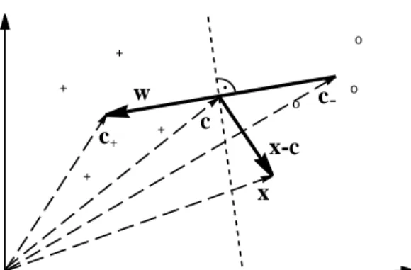
We are now in the position to describe a pattern recognition learning algorithm that is arguable one of the simplest possible. The basic idea is to compute the means of the two classes in feature space,
c+= 1 m+ X {i:yi=+1} xi, (6) c−= 1 m− X {i:yi=−1} xi, (7)
where m+and m− are the number of examples with positive and negative labels, re-spectively (see Figure 1). We then assign a new point x to the class whose mean is
o + + + + o o
c
+c-x-c
w
x
c
.Fig. 1. A simple geometric classification algorithm: given two classes of points (depicted by ‘o’
and ‘+’), compute their means c+, c−and assign a test pattern x to the one whose mean is closer. This can be done by looking at the dot product between x − c (where c = (c++ c−)/2) and w := c+− c−, which changes sign as the enclosed angle passes through π/2. Note that the corresponding decision boundary is a hyperplane (the dotted line) orthogonal to w (from [31]).
closer to it. This geometrical construction can be formulated in terms of dot products. Half-way in between c+and c−lies the point c := (c++ c−)/2. We compute the class of x by checking whether the vector connecting c and x encloses an angle smaller than
π/2 with the vector w := c+− c−connecting the class means, in other words
y = sgn ((x − c) · w)
y = sgn ((x − (c++ c−)/2) · (c+− c−))
= sgn ((x · c+) − (x · c−) + b). (8)
Here, we have defined the offset
b := 1 2 ¡ kc−k2− kc+k2 ¢ . (9)
It will be proved instructive to rewrite this expression in terms of the patterns xiin the input domain X . To this end, note that we do not have a dot product in X , all we have is the similarity measure k (cf. (5)). Therefore, we need to rewrite everything in terms of the kernel k evaluated on input patterns. To this end, substitute (6) and (7) into (8) to get the decision function
y = sgn 1 m+ X {i:yi=+1} (x · xi) − 1 m− X {i:yi=−1} (x · xi) + b = sgn 1 m+ X {i:yi=+1} k(x, xi) − 1 m− X {i:yi=−1} k(x, xi) + b . (10)
Similarly, the offset becomes b := 1 2 1 m2 − X {(i,j):yi=yj=−1} k(xi, xj) − 1 m2 + X {(i,j):yi=yj=+1} k(xi, xj) . (11) Let us consider one well-known special case of this type of classifier. Assume that the class means have the same distance to the origin (hence b = 0), and that k can be viewed as a density, i.e., it is positive and has integral 1,
Z X
k(x, x0)dx = 1 for all x0 ∈ X . (12)
In order to state this assumption, we have to require that we can define an integral on
X .
If the above holds true, then (10) corresponds to the so-called Bayes decision bound-ary separating the two classes, subject to the assumption that the two classes were gen-erated from two probability distributions that are correctly estimated by the Parzen
windows estimators of the two classes,
p1(x) := 1 m+ X {i:yi=+1} k(x, xi) (13) p2(x) := 1 m− X {i:yi=−1} k(x, xi). (14)
Given some point x, the label is then simply computed by checking which of the two,
p1(x) or p2(x), is larger, which directly leads to (10). Note that this decision is the best we can do if we have no prior information about the probabilities of the two classes. For further details, see [31].
The classifier (10) is quite close to the types of learning machines that we will be interested in. It is linear in the feature space, and while in the input domain, it is represented by a kernel expansion in terms of the training points. It is example-based in the sense that the kernels are centered on the training examples, i.e., one of the two arguments of the kernels is always a training example. The main points that the more sophisticated techniques to be discussed later will deviate from (10) are in the selection of the examples that the kernels are centered on, and in the weights that are put on the individual data in the decision function. Namely, it will no longer be the case that all training examples appear in the kernel expansion, and the weights of the kernels in the expansion will no longer be uniform. In the feature space representation, this statement corresponds to saying that we will study all normal vectors w of decision hyperplanes that can be represented as linear combinations of the training examples. For instance, we might want to remove the influence of patterns that are very far away from the decision boundary, either since we expect that they will not improve the generalization error of the decision function, or since we would like to reduce the computational cost of evaluating the decision function (cf. (10)). The hyperplane will then only depend on a subset of training examples, called support vectors.
2
Learning Pattern Recognition from Examples
With the above example in mind, let us now consider the problem of pattern recognition in a more formal setting ([37], [38]), following the introduction of [30]. In two-class pattern recognition, we seek to estimate a function
f : X → {±1} (15)
based on input-output training data (1). We assume that the data were generated inde-pendently from some unknown (but fixed) probability distribution P (x, y). Our goal is to learn a function that will correctly classify unseen examples (x, y), i.e., we want
f (x) = y for examples (x, y) that were also generated from P (x, y).
If we put no restriction on the class of functions that we choose our estimate f from, however, even a function which does well on the training data, e.g. by satisfying
f (xi) = yifor all i = 1, . . . , m, need not generalize well to unseen examples. To see this, note that for each function f and any test set (¯x1, ¯y1), . . . , (¯xm¯, ¯ym¯) ∈ RN×{±1}, satisfying {¯x1, . . . , ¯xm¯} ∩ {x1, . . . , xm} = {}, there exists another function f∗ such that f∗(xi) = f (xi) for all i = 1, . . . , m, yet f∗(¯xi) 6= f (¯xi) for all i = 1, . . . , ¯m. As we are only given the training data, we have no means of selecting which of the two functions (and hence which of the completely different sets of test label predictions) is preferable. Hence, only minimizing the training error (or empirical risk),
Remp[f ] = 1 m m X i=1 1 2|f (xi) − yi|, (16) does not imply a small test error (called risk), averaged over test examples drawn from the underlying distribution P (x, y),
R[f ] =
Z 1
2|f (x) − y| dP (x, y). (17) Statistical learning theory ([41], [37], [38], [39]), or VC (Vapnik-Chervonenkis) theory, shows that it is imperative to restrict the class of functions that f is chosen from to one which has a capacity that is suitable for the amount of available training data. VC theory provides bounds on the test error. The minimization of these bounds, which depend on both the empirical risk and the capacity of the function class, leads to the principle of
structural risk minimization ([37]). The best-known capacity concept of VC theory is
the VC dimension, defined as the largest number h of points that can be separated in all possible ways using functions of the given class. An example of a VC bound is the following: if h < m is the VC dimension of the class of functions that the learning machine can implement, then for all functions of that class, with a probability of at least 1 − η, the bound
R(f ) ≤ Remp(f ) + φ µ h m, log(η) m ¶ (18) holds, where the confidence term φ is defined as
φ µ h m, log(η) m ¶ = s h¡log2m h + 1 ¢ − log(η/4) m . (19)
Tighter bounds can be formulated in terms of other concepts, such as the annealed VC
entropy or the Growth function. These are usually considered to be harder to evaluate,
but they play a fundamental role in the conceptual part of VC theory ([38]). Alterna-tive capacity concepts that can be used to formulate bounds include the fat shattering
dimension ([2]).
The bound (18) deserves some further explanatory remarks. Suppose we wanted to learn a “dependency” where P (x, y) = P (x) · P (y), i.e., where the pattern x contains no information about the label y, with uniform P (y). Given a training sample of fixed size, we can then surely come up with a learning machine which achieves zero training error (provided we have no examples contradicting each other). However, in order to reproduce the random labelling, this machine will necessarily require a large VC di-mension h. Thus, the confidence term (19), increasing monotonically with h, will be large, and the bound (18) will not support possible hopes that due to the small training error, we should expect a small test error. This makes it understandable how (18) can hold independent of assumptions about the underlying distribution P (x, y): it always holds (provided that h < m), but it does not always make a nontrivial prediction — a bound on an error rate becomes void if it is larger than the maximum error rate. In order to get nontrivial predictions from (18), the function space must be restricted such that the capacity (e.g. VC dimension) is small enough (in relation to the available amount of data).
3
Hyperplane Classifiers
In the present section, we shall describe a hyperplane learning algorithm that can be performed in a dot product space (such as the feature space that we introduced previ-ously). As described in the previous section, to design learning algorithms, one needs to come up with a class of functions whose capacity can be computed.
[42] considered the class of hyperplanes
(w · x) + b = 0 w ∈ RN, b ∈ R, (20)
corresponding to decision functions
f (x) = sgn ((w · x) + b), (21)
and proposed a learning algorithm for separable problems, termed the Generalized
Por-trait, for constructing f from empirical data. It is based on two facts. First, among all
hyperplanes separating the data, there exists a unique one yielding the maximum margin of separation between the classes,
max
w,b min{kx − xik : x ∈ R
N, (w · x) + b = 0, i = 1, . . . , m}. (22) Second, the capacity decreases with increasing margin.
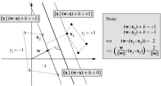
To construct this Optimal Hyperplane (cf. Figure 2), one solves the following opti-mization problem: minimize w,b 1 2kwk 2 subject to yi· ((w · xi) + b) ≥ 1, i = 1, . . . , m. (23)
.
w
{x
|
(w x) + b = 0
.
}
{x
|
(w x) + b = −1
.
}
{x
|
(w x) + b = +1
}
.
x
2x
1Note:
(w x
1) + b = +1
(w x
2) + b = −1
=> (w (x
1−x
2)) =
2
=>
(
||w||
w
(x
1−x
2) =
)
.
.
.
.
2
||w||
y
i= −1
y
i= +1
❍ ❍ ❍ ❍ ❍ ◆ ◆ ◆ ◆Fig. 2. A binary classification toy problem: separate balls from diamonds. The optimal hyperplane
is orthogonal to the shortest line connecting the convex hulls of the two classes (dotted), and intersects it half-way between the two classes. The problem is separable, so there exists a weight vector w and a threshold b such that yi· ((w · xi) + b) > 0 (i = 1, . . . , m). Rescaling w and b such that the point(s) closest to the hyperplane satisfy |(w · xi) + b| = 1, we obtain a canonical form (w, b) of the hyperplane, satisfying yi· ((w · xi) + b) ≥ 1. Note that in this case, the margin, measured perpendicularly to the hyperplane, equals 2/kwk. This can be seen by considering two points x1, x2on opposite sides of the margin, i.e., (w · x1) + b = 1, (w · x2) + b = −1, and
projecting them onto the hyperplane normal vector w/kwk (from [29]).
A way to solve (23) is through its Lagrangian dual: max α≥0(minw,bL(w, b, α)), (24) where L(w, b, α) = 1 2kwk 2− m X i=1 αi(yi· ((xi· w) + b) − 1) . (25) The Lagrangian L has to be minimized with respect to the primal variables w and
b and maximized with respect to the dual variables αi. For a nonlinear problem like (23), called the primal problem, there are several closely related problems of which the Lagrangian dual is an important one. Under certain conditions, the primal and dual problems have the same optimal objective values. Therefore, we can instead solve the dual which may be an easier problem than the primal. In particular, we will see in Section 4 that when working in feature spaces, solving the dual may be the only way to train SVM.
Let us try to get some intuition for this primal-dual relation. Assume ( ¯w, ¯b) is an
optimal solution of the primal with the optimal objective value γ = 12k ¯wk2. Thus, no (w, b) satisfies
1 2kwk
2< γ and y
With (26), there is ¯α ≥ 0 such that for all w, b 1 2kwk 2− γ − m X i=1 ¯ αi(yi· ((xi· w) + b) − 1) ≥ 0. (27)
We do not provide a rigorous proof here but details can be found in, for example, [5]. Note that for general convex programming this result requires some additional condi-tions on constraints which are now satisfied by our simple linear inequalities.
Therefore, (27) implies max
α≥0minw,bL(w, b, α) ≥ γ. (28) On the other hand, for any α,
min w,bL(w, b, α) ≤ L( ¯w, ¯b, α), so max α≥0minw,bL(w, b, α) ≤ maxα≥0L( ¯w, ¯b, α) = 1 2k ¯wk 2= γ. (29)
Therefore, with (28), the inequality in (29) becomes an equality. This property is the strong duality where the primal and dual have the same optimal objective value. In addition, putting ( ¯w, ¯b) into (27), with ¯αi ≥ 0 and yi· ((xi· ¯w) + ¯b) − 1 ≥ 0,
¯
αi· [yi((xi· ¯w) + ¯b) − 1] = 0, i = 1, . . . , m, (30) which is usually called the complementarity condition.
To simplify the dual, as L(w, b, α) is convex when α is fixed, for any given α,
∂ ∂bL(w, b, α) = 0, ∂ ∂wL(w, b, α) = 0, (31) leads to m X i=1 αiyi= 0 (32) and w = m X i=1 αiyixi. (33)
As α is now given, we may wonder what (32) means. From the definition of the La-grangian, ifPmi=1αiyi 6= 0, we can decrease −b
Pm
i=1αiyiin L(w, b, α) as much as we want. Therefore, by substituting (33) into (24), the dual problem can be written as
max α≥0 (Pm i=1αi−12 Pm i,j=1αiαjyiyj(xi· xj) if Pm i=1αiyi = 0, −∞ if Pmi=1αiyi 6= 0. (34)
As −∞ is definitely not the maximal objective value of the dual, the dual optimal so-lution does not happen whenPmi=1αiyi 6= 0. Therefore, the dual problem is simplified to finding multipliers αiwhich
maximize α∈Rm m X i=1 αi−1 2 m X i,j=1 αiαjyiyj(xi· xj) (35) subject to αi≥ 0, i = 1, . . . , m, and m X i=1 αiyi= 0. (36)
This is the dual SVM problem that we usually refer to. Note that (30), (32), αi≥ 0∀i, and (33), are called the Karush-Kuhn-Tucker (KKT) optimality conditions of the primal problem. Except an abnormal situation where all optimal αiare zero, b can be computed using (30).
The discussion from (31) to (33) implies that we can consider a different form of dual problem: maximize w,b,α≥0 L(w, b, α) subject to ∂ ∂bL(w, b, α) = 0, ∂ ∂wL(w, b, α) = 0. (37)
This is the so called Wolfe dual for convex optimization, which is a very early work in duality [45]. For convex and differentiable problems, it is equivalent to the Lagrangian dual though the derivation of the Lagrangian dual more easily shows the strong duality results. Some notes about the two duals are in, for example, [3, Section 5.4].
Following the above discussion, the hyperplane decision function can be written as
f (x) = sgn Ãm X i=1 yiαi· (x · xi) + b ! . (38)
The solution vector w thus has an expansion in terms of a subset of the training pat-terns, namely those patterns whose αiis non-zero, called Support Vectors. By (30), the Support Vectors lie on the margin (cf. Figure 2). All remaining examples of the training set are irrelevant: their constraint (23) does not play a role in the optimization, and they do not appear in the expansion (33). This nicely captures our intuition of the problem: as the hyperplane (cf. Figure 2) is completely determined by the patterns closest to it, the solution should not depend on the other examples.
The structure of the optimization problem closely resembles those that typically arise in Lagrange’s formulation of mechanics. Also there, often only a subset of the constraints become active. For instance, if we keep a ball in a box, then it will typically roll into one of the corners. The constraints corresponding to the walls which are not touched by the ball are irrelevant, the walls could just as well be removed.
Seen in this light, it is not too surprising that it is possible to give a mechanical in-terpretation of optimal margin hyperplanes ([9]): If we assume that each support vector xiexerts a perpendicular force of size αiand sign yion a solid plane sheet lying along the hyperplane, then the solution satisfies the requirements of mechanical stability. The
constraint (32) states that the forces on the sheet sum to zero; and (33) implies that the torques also sum to zero, viaPixi× yiαi· w/kwk = w × w/kwk = 0.
There are theoretical arguments supporting the good generalization performance of the optimal hyperplane ([41], [37], [4], [33], [44]). In addition, it is computationally attractive, since it can be constructed by solving a quadratic programming problem.
4
Optimal Margin Support Vector Classifiers
We now have all the tools to describe support vector machines ([38], [31]). Everything in the last section was formulated in a dot product space. We think of this space as the feature space H described in Section 1. To express the formulas in terms of the input patterns living in X , we thus need to employ (5), which expresses the dot product of bold face feature vectors x, x0in terms of the kernel k evaluated on input patterns x, x0,
k(x, x0) = (x · x0). (39)
This can be done since all feature vectors only occurred in dot products. The weight vector (cf. (33)) then becomes an expansion in feature space,1 and will thus typically no longer correspond to the image of a single vector from input space. We thus obtain decision functions of the more general form (cf. (38))
f (x) = sgn Ãm X i=1 yiαi· (Φ(x) · Φ(xi)) + b ! = sgn Ãm X i=1 yiαi· k(x, xi) + b ! , (40)
and the following quadratic program (cf. (35)):
maximize α∈Rm W (α) = m X i=1 αi−1 2 m X i,j=1 αiαjyiyjk(xi, xj) (41) subject to αi≥ 0, i = 1, . . . , m, and m X i=1 αiyi= 0. (42)
Working in the feature space somewhat forces us to solve the dual problem instead of the primal. The dual problem has the same number of variables as the number of training data. However, the primal problem may have a lot more (even infinite) variables depending on the dimensionality of the feature space (i.e. the length of Φ(x)). Though our derivation of the dual problem in Section 3 considers problems in finite-dimensional spaces, it can be directly extended to problems in Hilbert spaces [20].
1This constitutes a special case of the so-called representer theorem, which states that under fairly general conditions, the minimizers of objective functions which contain a penalizer in terms of a norm in feature space will have kernel expansions ([43], [31]).
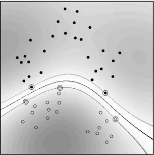
Fig. 3. Example of a Support Vector classifier found by using a radial basis function kernel k(x, x0) = exp(−kx − x0k2). Both coordinate axes range from -1 to +1. Circles and disks
are two classes of training examples; the middle line is the decision surface; the outer lines pre-cisely meet the constraint (23). Note that the Support Vectors found by the algorithm (marked by extra circles) are not centers of clusters, but examples which are critical for the given classifica-tion task. Grey values code the modulus of the argumentPmi=1yiαi· k(x, xi) + b of the decision function (40) (from [29]).)
5
Kernels
We now take a closer look at the issue of the similarity measure, or kernel, k. In this section, we think of X as a subset of the vector space RN, (N ∈ N), endowed with the canonical dot product (3).
5.1 Product Features
Suppose we are given patterns x ∈ RN where most information is contained in the dth order products (monomials) of entries [x]jof x,
[x]j1· · · [x]jd, (43) where j1, . . . , jd ∈ {1, . . . , N }. In that case, we might prefer to extract these product features, and work in the feature space H of all products of d entries. In visual recog-nition problems, where images are often represented as vectors, this would amount to extracting features which are products of individual pixels.
For instance, in R2, we can collect all monomial feature extractors of degree 2 in the nonlinear map
Φ : R2→ H = R3 (44)
([x]1, [x]2) 7→ ([x]21, [x]22, [x]1[x]2). (45) This approach works fine for small toy examples, but it fails for realistically sized prob-lems: for N -dimensional input patterns, there exist
NH= (N + d − 1)!
d!(N − 1)! (46)
different monomials (43), comprising a feature space H of dimensionality NH. For instance, already 16 × 16 pixel input images and a monomial degree d = 5 yield a dimensionality of 1010.
In certain cases described below, there exists, however, a way of computing dot
products in these high-dimensional feature spaces without explicitly mapping into them:
by means of kernels nonlinear in the input space RN. Thus, if the subsequent process-ing can be carried out usprocess-ing dot products exclusively, we are able to deal with the high dimensionality.
5.2 Polynomial Feature Spaces Induced by Kernels
In order to compute dot products of the form (Φ(x) · Φ(x0)), we employ kernel repre-sentations of the form
k(x, x0) = (Φ(x) · Φ(x0)), (47) which allow us to compute the value of the dot product in H without having to carry out the map Φ. This method was used by Boser et al. to extend the Generalized
Por-trait hyperplane classifier [41] to nonlinear Support Vector machines [8]. Aizerman et
al. called H the linearization space, and used in the context of the potential function classification method to express the dot product between elements of H in terms of elements of the input space [1].
What does k look like for the case of polynomial features? We start by giving an example ([38]) for N = d = 2. For the map
Φ2: ([x]1, [x]2) 7→ ([x]21, [x]22, [x]1[x]2, [x]2[x]1), (48) dot products in H take the form
(Φ2(x) · Φ2(x0)) = [x]21[x0]21+ [x]22[x0]22+ 2[x]1[x]2[x0]1[x0]2= (x · x0)2, (49) i.e., the desired kernel k is simply the square of the dot product in input space. Note that it is possible to modify (x · x0)dsuch that it maps into the space of all monomials up to degree d, defining ([38])
5.3 Examples of Kernels
When considering feature maps, it is also possible to look at things the other way around, and start with the kernel. Given a kernel function satisfying a mathematical condition termed positive definiteness, it is possible to construct a feature space such that the kernel computes the dot product in that feature space. This has been brought to the attention of the machine learning community by [1], [8], and [38]. In functional analysis, the issue has been studied under the heading of Reproducing kernel Hilbert
space (RKHS).
Besides (50), a popular choice of kernel is the Gaussian radial basis function ([1])
k(x, x0) = exp¡−γkx − x0k2¢. (51) An illustration is in Figure 3. For an overview of other kernels, see [31].
6
ν-Soft Margin Support Vector Classifiers
In practice, a separating hyperplane may not exist, e.g. if a high noise level causes a large overlap of the classes. To allow for the possibility of examples violating (23), one introduces slack variables ([15], [38], [32])
ξi≥ 0, i = 1, . . . , m (52)
in order to relax the constraints to
yi· ((w · xi) + b) ≥ 1 − ξi, i = 1, . . . , m. (53) A classifier which generalizes well is then found by controlling both the classifier ca-pacity (via kwk) and the sum of the slacksPiξi. The latter is done as it can be shown to provide an upper bound on the number of training errors which leads to a convex optimization problem.
One possible realization,called C-SVC, of a soft margin classifier is minimizing the objective function τ (w, ξ) = 1 2kwk 2+ C m X i=1 ξi (54)
subject to the constraints (52) and (53), for some value of the constant C > 0 deter-mining the trade-off. Here and below, we use boldface Greek letters as a shorthand for corresponding vectors ξ = (ξ1, . . . , ξm). Incorporating kernels, and rewriting it in terms of Lagrange multipliers, this again leads to the problem of maximizing (41), subject to the constraints
0 ≤ αi≤ C, i = 1, . . . , m, and m X i=1
αiyi= 0. (55)
The only difference from the separable case is the upper bound C on the Lagrange mul-tipliers αi. This way, the influence of the individual patterns (which could be outliers) gets limited. As above, the solution takes the form (40).
Another possible realization,called ν-SVC of a soft margin variant of the optimal hyperplane uses the ν-parameterization ([32]). In it, the parameter C is replaced by a parameter ν ∈ [0, 1] which is the lower and upper bound on the number of examples that are support vectors and that lie on the wrong side of the hyperplane, respectively.
As a primal problem for this approach, termed the ν-SV classifier, we consider minimize w∈H,ξ∈Rm,ρ,b∈R τ (w, ξ, ρ) = 1 2kwk 2− νρ + 1 m m X i=1 ξi (56) subject to yi(hxi, wi + b) ≥ ρ − ξi, i = 1, . . . , m (57) and ξi≥ 0, ρ ≥ 0. (58)
Note that no constant C appears in this formulation; instead, there is a parameter ν, and also an additional variable ρ to be optimized. To understand the role of ρ, note that for
ξ = 0, the constraint (57) simply states that the two classes are separated by the margin
2ρ/kwk.
To explain the significance of ν, let us first introduce the term margin error: by this, we denote training points with ξi > 0. These are points which either are errors, or lie within the margin. Formally, the fraction of margin errors is
Rρemp[g] := 1
m|{i|yig(xi) < ρ}| . (59)
Here, g is used to denote the argument of the sign in the decision function (40): f = sgn ◦g. We are now in a position to state a result that explains the significance of ν.
Proposition 1 ([32]). Suppose we run ν-SVC with kernel function k on some data with
the result that ρ > 0. Then
(i) ν is an upper bound on the fraction of margin errors (and hence also on the fraction of training errors).
(ii) ν is a lower bound on the fraction of SVs.
(iii) Suppose the data (x1, y1), . . . , (xm, ym) were generated iid from a distribution Pr(x, y) = Pr(x) Pr(y|x), such that neither Pr(x, y = 1) nor Pr(x, y = −1) con-tains any discrete component. Suppose, moreover, that the kernel used is analytic and non-constant. With probability 1, asymptotically, ν equals both the fraction of SVs and the fraction of margin errors.
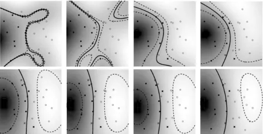
Before we get into the technical details of the dual derivation, let us take a look at a toy example illustrating the influence of ν (Figure 4). The corresponding fractions of SVs and margin errors are listed in table 1.
Let us next derive the dual of the ν-SV classification algorithm. We consider the Lagrangian L(w, ξ, b, ρ, α, β, δ) = 1 2kwk 2− νρ + 1 m m X i=1 ξi − m X i=1 (αi(yi(hxi, wi + b) − ρ + ξi) + βiξi− δρ), (60)
Fig. 4. Toy problem (task: to separate circles from disks) solved using ν-SV classification, with
parameter values ranging from ν = 0.1 (top left) to ν = 0.8 (bottom right). The larger we make
ν, the more points are allowed to lie inside the margin (depicted by dotted lines). Results are
shown for a Gaussian kernel, k(x, x0) = exp(−kx − x0k2) (from [31]).
Table 1. Fractions of errors and SVs, along with the margins of class separation, for the toy
example in Figure 4.
Note that ν upper bounds the fraction of errors and lower bounds the fraction of SVs, and that increasing ν, i.e., allowing more errors, increases the margin.
ν 0.1 0.2 0.3 0.4 0.5 0.6 0.7 0.8
fraction of errors 0.00 0.07 0.25 0.32 0.39 0.50 0.61 0.71 fraction of SVs 0.29 0.36 0.43 0.46 0.57 0.68 0.79 0.86 margin ρ/kwk 0.005 0.018 0.115 0.156 0.364 0.419 0.461 0.546
using multipliers αi, βi, δ ≥ 0. This function has to be minimized with respect to the primal variables w, ξ, b, ρ, and maximized with respect to the dual variables α, β, δ. Following the same derivation in (31)–(33), we compute the corresponding partial derivatives and set them to 0, obtaining the following conditions:
w = m X i=1 αiyixi, (61) αi+ βi= 1/m, (62) m X i=1 αiyi= 0, (63) m X i=1 αi− δ = ν. (64)
Again, in the SV expansion (61), the αithat are non-zero correspond to a constraint (57) which is precisely met.
Substituting (61) and (62) into L, using αi, βi, δ ≥ 0, and incorporating kernels for dot products, leaves us with the following quadratic optimization problem for ν-SV classification: maximize α∈Rm W (α) = − 1 2 m X i,j=1 αiαjyiyjk(xi, xj) (65) subject to 0 ≤ αi≤ 1 m, (66) m X i=1 αiyi= 0, (67) m X i=1 αi≥ ν. (68)
As above, the resulting decision function can be shown to take the form
f (x) = sgn à m X i=1 αiyik(x, xi) + b ! . (69)
Compared with the C-SVC dual ((41), (55)), there are two differences. First, there is an additional constraint (68). Second, the linear termPmi=1αino longer appears in the objective function (65). This has an interesting consequence: (65) is now quadratically homogeneous in α. It is straightforward to verify that the same decision function is obtained if we start with the primal function
τ (w, ξ, ρ) = 1 2kwk 2+ C Ã −νρ + 1 m m X i=1 ξi ! , (70)
i.e., if one does use C [31].
The computation of the threshold b and the margin parameter ρ will be discussed in Section 7.4.
A connection to standard SV classification, and a somewhat surprising interpreta-tion of the regularizainterpreta-tion parameter C, is described by the following result:
Proposition 2 (Connection ν-SVC — C-SVC [32]). If ν-SV classification leads to
ρ > 0, then C-SV classification, with C set a priori to 1/mρ, leads to the same decision
function.
For further details on the connection between ν-SVMs and C-SVMs, see [16, 6]. By considering the optimal α as a function of parameters, a complete account is as follows:
Proposition 3 (Detailed connection ν-SVC — C-SVC [11]).Pmi=1αi/(Cm) by the
C-SVM is a well defined decreasing function of C. We can define
lim C→∞
Pm i=1αi
Cm = νmin≥ 0 and limC→0 Pm
i=1αi
Cm = νmax≤ 1. (71)
1. νmax= 2 min(m+, m−)/m.
2. For any ν > νmax, the dual ν-SVM is infeasible. That is, the set of feasible points is
empty. For any ν ∈ (νmin, νmax], the optimal solution set of dual ν-SVM is the same
as that of either one or some C-SVM where these C form an interval. In addition, the optimal objective value of ν-SVM is strictly positive. For any 0 ≤ ν ≤ νmin,
dual ν-SVM is feasible with zero optimal objective value. 3. If the kernel matrix is positive definite, then νmin= 0.
Therefore, for a given problem and kernel, there is an interval [νmin, νmax] of admissible values for ν, with 0 ≤ νmin ≤ νmax≤ 1. An illustration of the relation between ν and
C is in Figure 5. 0 0.1 0.2 0.3 0.4 0.5 0.6 0.7 0.8 0.9 -3 -2 -1 0 1 2 3 4 5 ν log10C
Fig. 5. The relation between ν and C (using the RBF kernel on the problemaustralianfrom the Statlog collection [25])
It has been noted that ν-SVMs have an interesting interpretation in terms of reduced
convex hulls [16, 6]. One can show that for separable problems, one can obtain the
opti-mal margin separating hyperplane by forming the convex hulls of both classes, finding the shortest connection between the two convex hulls (since the problem is separable, they are disjoint), and putting the hyperplane halfway along that connection, orthogonal to it. If a problem is non-separable, however, the convex hulls of the two classes will no longer be disjoint. Therefore, it no longer makes sense to search for the shortest line connecting them. In this situation, it seems natural to reduce the convex hulls in size, by limiting the size of the coefficients ciin the convex sets
C± := ( X yi=±1 cixi ¯ ¯ ¯ ¯ ¯ X yi=±1 ci= 1, ci≥ 0 ) . (72)
to some value ν ∈ (0, 1). Intuitively, this amounts to limiting the influence of individual points. It is possible to show that the ν-SVM formulation solves the problem of finding the hyperplane orthogonal to the closest line connecting the reduced convex hulls [16]. We now move on to another aspect of soft margin classification. When we intro-duced the slack variables, we did not attempt to justify the fact that in the objective function, we used a penalizerPmi=1ξi. Why not use another penalizer, such as
Pm i=1ξ
p i, for some p ≥ 0 [15]? For instance, p = 0 would yield a penalizer that exactly counts the number of margin errors. Unfortunately, however, it is also a penalizer that leads to a combinatorial optimization problem. Penalizers yielding optimization problems that are particularly convenient, on the other hand, are obtained for p = 1 and p = 2. By default, we use the former, as it possesses an additional property which is statistically attractive. As the following proposition shows, linearity of the target function in the slack variables ξileads to a certain “outlier” resistance of the estimator. As above, we use the shorthand xifor Φ(xi).
Proposition 4 (Resistance of SV classification [32]). Suppose w can be expressed in
terms of the SVs which are not at bound,
w =
m X i=1
γixi (73)
with γi 6= 0 only if αi ∈ (0, 1/m) (where the αi are the coefficients of the dual
solu-tion). Then local movements of any margin error xj parallel to w do not change the
hyperplane.2
This result is about the stability of classifiers. Results have also shown that in general
p = 1 leads to fewer support vectors. Further results in support of the p = 1 case can
be seen in [34, 36].
Although proposition 1 shows that ν possesses an intuitive meaning, it is still un-clear how to choose ν for a learning task. [35] proves that given ¯R, a close upper bound
on the expected optimal Bayes risk, an asymptotically good estimate of the optimal value of ν is 2 ¯R:
Proposition 5. If R[f ] is the expected risk defined in (17),
Rp:= inf
f R[f ], (74)
and the kernel used by ν-SVM is universal, then for all ν > 2Rpand all ² > 0, there
exists a constant c > 0 such that
P (T = {(x1, y1), . . . , (xm, ym)} | R[fTν] ≤ ν − Rp+ ²) ≥ 1 − e−cm. (75)
Quite a few popular kernels such as the Gaussian are universal. The definition of a universal kernel can be seen in [35]. Here, fTν is the decision function obtained by training ν-SVM on the data set T .
2
Note that the perturbation of the point is carried out in feature space. What it precisely corre-sponds to in input space therefore depends on the specific kernel chosen.
Therefore, given an upper bound ¯R on Rp, the decision function with respect to ν = 2 ¯R almost surely achieves a risk not larger than Rp+ 2( ¯R − Rp).
The selection of ν and kernel parameters can be done by estimating the performance of support vector binary classifiers on data not yet observed. One such performance esti-mate is the leave-one-out error, which is an almost unbiased estiesti-mate of the generaliza-tion performance [22]. To compute this performance metric, a single point is excluded from the training set, and the classifier is trained using the remaining points. It is then determined whether this new classifier correctly labels the point that was excluded. The process is repeated over the entire training set. Although theoretically attractive, this estimate obviously entails a large computational cost.
Three estimates of the leave-one-out error for the ν-SV learning algorithm are pre-sented in [17]. Of these three estimates, the general ν-SV bound is an upper bound on the leave-one-out error, the restricted ν-SV estimate is an approximation that assumes the sets of margin errors and support vectors on the margin to be constant, and the
max-imized target estimate is an approximation that assumes the sets of margin errors and
non-support vectors not to decrease. The derivation of the general ν-SV bound takes a form similar to an upper bound described in [40] for the C-SV classifier, while the restricted ν-SV estimate is based on a similar C-SV estimate proposed in [40, 26]: both these estimates are based on the geometrical concept of the span, which is (roughly speaking) a measure of how easily a particular point in the training sample can be replaced by the other points used to define the classification function. No analogous method exists in the C-SV case for the maximized target estimate.
7
Implementation of ν-SV Classifiers
We change the dual form of ν-SV classifiers to be a minimization problem: minimize α∈Rm W (α) = 1 2 m X i,j=1 αiαjyiyjk(xi, xj) subject to 0 ≤ αi≤ 1 m, (76) m X i=1 αiyi= 0, m X i=1 αi= ν. (77)
[11] proves that for any given ν, there is at least an optimal solution which satisfies
eTα = ν. Therefore, it is sufficient to solve a simpler problem with the equality con-straint (77).
Similar to C-SVC, the difficulty of solving (76) is that yiyjk(xi, xj) are in gen-eral not zero. Thus, for large data sets, the Hessian (second derivative) matrix of the objective function cannot be stored in the computer memory, so traditional optimiza-tion methods such as Newton or quasi Newton cannot be directly used. Currently, the decomposition method is the most used approach to conquer this difficulty. Here, we present the implementation in [11], which modifies the procedure for C-SVC.
7.1 The Decomposition Method
The decomposition method is an iterative process. In each step, the index set of variables is partitioned to two sets B and N , where B is the working set. Then, in that iteration variables corresponding to N are fixed while a sub-problem on variables corresponding to B is minimized. The procedure is as follows:
Algorithm 1 (Decomposition method)
1. Given a numberq ≤ las the size of the working set. Findα1as an initial feasible
solution of (76). Setk = 1.
2. If αk is an optimal solution of (76), stop. Otherwise, find a working set B ⊂
{1, . . . , l}whose size isq. DefineN ≡ {1, . . . , l}\BandαkB andαkN to be
sub-vectors ofαkcorresponding toBandN, respectively.
3. Solve the following sub-problem with the variableαB:
minimize αB∈Rq 1 2 X i∈B,j∈B αiαjyiyjk(xi, xj) + X i∈B,j∈N αiαkjyiyjk(xi, xj) subject to 0 ≤ αi≤ 1 m, i ∈ B, (78) X i∈B αiyi = − X i∈N αk iyi, (79) X i∈B αi= ν − X i∈N αki. (80)
4. Setαk+1B to be the optimal solution of (78) andαk+1N ≡ αkN. Setk ← k + 1and
goto Step 2.
Note that B is updated in each iteration. To simplify the notation, we simply use B instead of Bk.
7.2 Working Set Selection
An important issue of the decomposition method is the selection of the working set B. Here, we consider an approach based on the violation of the KKT condition. Similar to (30), by putting (61) into (57), one of the KKT conditions is
αi· [yi( m X j=1
αjK(xi, xj) + b) − ρ + ξi] = 0, i = 1, . . . , m. (81)
Using 0 ≤ αi≤ m1, (81) can be rewritten as: m X j=1 αjyiyjk(xi, xj) + byi− ρ ≥ 0, if αi< 1 m, m X j=1 αjyiyjk(xi, xj) + byi− ρ ≤ 0, if αi> 0. (82)
That is, an α is optimal for the dual problem (76) if and only if α is feasible and satisfies (81). Using the property that yi= ±1 and representing ∇W (α)i =
Pm
j=1αjyiyjK(xi, xj), (82) can be further written as
max i∈I1 up(α) ∇W (α)i≤ ρ − b ≤ min i∈I1 low(α) ∇W (α)iand max i∈I−1 up(α) ∇W (α)i≤ ρ + b ≤ min i∈I−1 low(α) ∇W (α)i, (83) where I1 up(α) := {i | αi> 0, yi= 1}, Ilow1 (α) := {i | αi < 1 m, yi= 1}, (84) and I−1 up(α) := {i | αi < 1 m, yi= −1}, I −1 low(α) := {i | αi> 0, yi= −1}. (85) We call any (i, j) ∈ Iup1 (α) × Ilow1 (α) or Iup−1(α) × Ilow−1(α) satisfying
yi∇W (α)i> yj∇W (α)j (86) a violating pair as (83) is not satisfied. When α is not optimal yet, if any such a violating pair is included in B, the optimal objective value of (78) is small than that at αk. Therefore, the decomposition procedure has its objective value strictly decreasing from one iteration to the next.
Therefore, a natural choice of B is to select all pairs which violate (83) the most. To be more precise, we can set q to be an even integer and sequentially select q/2 pairs
{(i1, j1), . . . , (iq/2, jq/2)} from ∈ Iup1 (α) × Ilow1 (α) or Iup−1(α) × Ilow−1(α) such that
yi1∇W (α)i1− yj1∇W (α)j1≥ · · · ≥ yiq/2∇W (α)iq/2− yjq/2∇W (α)jq/2. (87) This working set selection is merely an extension of that for C-SVC. The main difference is that for C-SVM, (83) becomes only one inequality with b. Due to this similarity, we believe that the convergence analysis of C-SVC [21] can be adapted here though detailed proofs have not been written and published.
[11] considers the same working set selection. However, following the derivation for C-SVC in [19], it is obtained using the concept of feasible directions in constrained optimization. We feel that a derivation from the violation of the KKT condition is more intuitive.
7.3 SMO-type Implementation
The Sequential Minimal Optimization (SMO) algorithm [28] is an extreme of the de-composition method where, for C-SVC, the working set is restricted to only two el-ements. The main advantage is that each two-variable sub-problem can be analyti-cally solved, so numerical optimization software are not needed. For this method, at least two elements are required for the working set. Otherwise, the equality constraint
P
i∈Bαiyi= − P
j∈Nαkjyjleads to a fixed optimal objective value of the sub-problem. Then, the decomposition procedure stays at the same point.
Now the dual of ν-SVC possesses two inequalities, so we may think that more elements are needed for the working set. Indeed, two elements are still enough for the case of ν-SVC. Note that (79) and (80) can be rewritten as
X i∈B,yi=1 αiyi= ν 2− X i∈N,yi=1 αk iyiand X i∈B,yi=−1 αiyi= ν 2− X i∈N,yi=−1 αk iyi. (88)
Thus, if (i1, j1) are selected as the working set selection using (87), yi1 = yj1, so
(88) reduces to only one equality with two variables. Then, the sub-problem is still guaranteed to be smaller than that at αk.
The comparison in [11] shows that using C and ν with the connection in proposition 3 and equivalent stopping condition, the performance of the SMO-type implementation described here for C-SVM and ν-SVM are comparable.
7.4 The Calculation of b and ρ and Stopping Criteria
If at an optimal solution, 0 < αi < 1/m and yi = 1, then i ∈ Iup1 (α) and Ilow1 (α). Thus, ρ − b = ∇W (α)i. Similarly, if there is another 0 < αj < 1/m and yj = −1, then ρ + b = ∇W (α)j. Thus, solving two equalities gives b and ρ. In practice, we average W (α)ito avoid numerical errors:
ρ − b = P 0<αi<m1,yi=1∇W (α)i P 0<αi<m1,yi=11 , (89)
If there are no components such that 0 < αi < 1/m, ρ − b (and ρ + b) can be any number in the interval formed by (83). A common way is to select the middle point and then still solves two linear equations
The stopping condition of the decomposition method can easily follow the new form of the optimality condition (83):
max¡− min i∈I1 low(α) ∇W (α)i+ max i∈I1 up(α) ∇W (α)i, − min i∈I−1 low(α) ∇W (α)i+ max i∈I−1 up(α) ∇W (α)i ¢ < ², (90)
where ² > 0 is a chosen stopping tolerance.
8
Multi-Class ν-SV Classifiers
Though SVM was originally designed for two-class problems, several approaches have been developed to extend SVM for multi-class data sets. In this section, we discuss the extension of the “one-against-one” approach for multi-class ν-SVM.
Most approaches for multi-class SVM decompose the data set to several binary problems. For example, the “one-against-one” approach trains a binary SVM for any
two classes of data and obtains a decision function. Thus, for a k-class problem, there are k(k−1)/2 decision functions. In the prediction stage, a voting strategy is used where the testing point is designated to be in a class with the maximum number of votes. In [18], it was experimentally shown that for general problems, using C-SV classifier, various multi-class approaches give similar accuracy. However, the “one-against-one” method is more efficient for training. Here, we will focus on extending it for ν-SVM.
Multi-class methods must be considered together with parameter-selection strate-gies. That is, we search for appropriate C and kernel parameters for constructing a better model. In the following, we restrict the discussion on only the Gaussian (radius basis function) kernel k(xi, xj) = e−γkxi−xjk
2
, so the kernel parameter is γ. With the parameter selection considered, there are two ways to implement the “one-against-one” method: First, for any two classes of data, the parameter selection is conducted to have the best (C, γ). Thus, for the best model selected, each decision function has its own (C, γ). For experiments here, the parameter selection of each binary SVM is by a five-fold cross-validation. The second way is that for each (C, γ), an evaluation criterion (e.g. cross-validation) combining with the “one-against-one” method is used for estimating the performance of the model. A sequence of pre-selected (C, γ) is tried to select the best model. Therefore, for each model, k(k − 1)/2 decision functions share the same C and γ.
It is not very clear which one of the two implementations is better. On one hand, a single parameter set may not be uniformly good for all k(k − 1)/2 decision functions. On the other hand, as the overall accuracy is the final consideration, one parameter set for one decision function may lead to over-fitting. [14] is the first to compare the two approaches using C-SVM, where the preliminary results show that both give similar accuracy.
For ν-SVM, each binary SVM using data from the ith and the jth classes has an admissible interval [νminij , νij
max], where νmaxij = 2 min(mi, mj)/(mi+ mj) according to proposition 3. Here mi and mj are the number of data points in the ith and jth classes, respectively. Thus, if all k(k − 1)/2 decision functions share the same ν, the admissible interval is
[max i6=j ν
ij
min, mini6=j νmaxij ]. (91) This set is non-empty if the kernel matrix is positive definite. The reason is that proposi-tion 3 implies νminij = 0, ∀i 6= j, so mini6=jνmaxij = 0. Therefore, unlike C of C-SVM, which has a large valid range [0, ∞), for ν-SVM, we worry that the admissible interval may be too small. For example, if the data set is highly unbalanced, mini6=jνminij is very small.
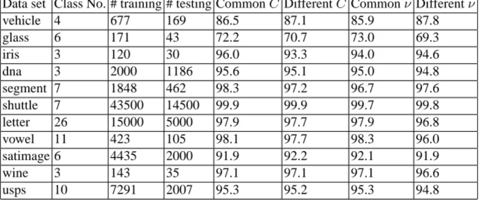
We redo the same comparison as that in [14] for ν-SVM. Results are in Table 2. We consider multi-class problems tested in [18], where most of them are from the statlog collection [25]. Except data sets dna, shuttle, letter, satimage, and usps, where test sets are available, we separate each problem to 80% training and 20% testing. Then, cross validation are conducted only on the training data. All other settings such as data scaling are the same as those in [18]. Experiments are conducted using LIBSVM [10], which solves both C-SVM and ν-SVM.
Results in Table 2 show no significant difference among the four implementations. Note that some problems (e.g. shuttle) are highly unbalanced so the admissible interval
(91) is very small. Surprisingly, from such intervals, we can still find a suitable ν which leads to a good model. This preliminary experiment indicates that in general the use of “one-against-one” approach for multi-class ν-SVM is viable.
Table 2. Test accuracy (in percentage) of multi-class data sets by C-SVM and ν-SVM. The
columns “Common C”, “Different C”, “Common ν”, “Different ν” are testing accuracy of using the same and different (C,γ), (or (ν,γ)) for all k(k − 1)/2 decision functions. The validation is conducted on the following points of (C,γ): [2−5, 2−3, . . . , 215] × [2−15, 2−13, . . . , 23]. For ν-SVM, the range of γ is the same but we validate a 10-point discretization of ν in the interval (91) or [νijmin, ν
ij
max], depending on whether k(k − 1)/2 decision functions share the same parameters
or not. For small problems (number of training data ≤ 1000), we do cross validation five times, and then average the testing accuracy.
Data set Class No. # training # testing Common C Different C Common ν Different ν
vehicle 4 677 169 86.5 87.1 85.9 87.8 glass 6 171 43 72.2 70.7 73.0 69.3 iris 3 120 30 96.0 93.3 94.0 94.6 dna 3 2000 1186 95.6 95.1 95.0 94.8 segment 7 1848 462 98.3 97.2 96.7 97.6 shuttle 7 43500 14500 99.9 99.9 99.7 99.8 letter 26 15000 5000 97.9 97.7 97.9 96.8 vowel 11 423 105 98.1 97.7 98.3 96.0 satimage 6 4435 2000 91.9 92.2 92.1 91.9 wine 3 143 35 97.1 97.1 97.1 96.6 usps 10 7291 2007 95.3 95.2 95.3 94.8
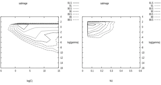
We also present the contours of C-SVM and ν-SVM in Figure 8 using the approach that all decision functions share the same (C, γ). In the contour of C-SVM, the x-axis and y-x-axis are log2C and log2γ, respectively. For ν-SVM, the x-axis is ν in the interval (91). Clearly, the good region of using ν-SVM is smaller. This confirms our concern earlier, which motivated us to conduct experiments in this section. Fortunately, points in this smaller good region still lead to models that are competitive with those by
C-SVM.
There are some ways to enlarge the admissible interval of ν. A work to extend algorithm to the case of very small values of ν by allowing negative margins is [27]. For the upper bound, according to the above proposition 3, if the classes are balanced, then the upper bound is 1. This leads to the idea to modify the algorithm by adjusting the cost function such that the classes are balanced in terms of the cost, even if they are not in terms of the mere numbers of training examples. An earlier discussion on such formulations is at [12]. For example, we can consider the following formulation:
minimize w∈H,ξ∈Rm,ρ,b∈R τ (w, ξ, ρ) = 1 2kwk 2− νρ + 1 2m+ X i:yi=1 ξi+ 1 2m− X i:yi=−1 ξi subject to yi(hxi, wi + b) ≥ ρ − ξi, and ξi≥ 0, ρ ≥ 0.
satimage 91.5 91 90.5 90 89.5 89 88.5 -5 0 5 10 15 log(C) -16 -14 -12 -10 -8 -6 -4 -2 0 2 4 log(gamma) satimage 91.5 91 90.5 90 89.5 89 88.5 0 0.1 0.2 0.3 0.4 0.5 0.6 NU -16 -14 -12 -10 -8 -6 -4 -2 0 2 4 log(gamma)
Fig. 6. 5-fold cross-validation accuracy of the data set satimage. Left: C-SVM, Right: ν-SVM
The dual is maximize α∈Rm W (α) = − 1 2 m X i,j=1 αiαjyiyjk(xi, xj) subject to 0 ≤ αi≤ 1 2m+, if yi= 1, 0 ≤ αi≤ 1 2m− , if yi = −1, m X i=1 αiyi= 0, m X i=1 αi≥ ν.
Clearly, when all αiequals its corresponding upper bound, α is a feasible solution with Pm i=1αi = 1 . Another possibility is minimize w∈H,ξ∈Rm,ρ,b∈R τ (w, ξ, ρ) = 1 2kwk 2− νρ + 1 2 min(m+, m−) m X i=1 ξi subject to yi(hxi, wi + b) ≥ ρ − ξi, and ξi≥ 0, ρ ≥ 0.
The dual is maximize α∈Rm W (α) = − 1 2 m X i,j=1 αiαjyiyjk(xi, xj) subject to 0 ≤ αi≤ 1 2 min(m+, m−) , m X i=1 αiyi= 0, m X i=1 αi≥ ν.
Then, the largest admissible ν is 1.
A slight modification of the implementation in Section 7 for the above formulations is in [13].
9
Applications of ν-SV Classifiers
Researchers have applied ν-SVM on different applications. Some of them feel that it is easier and more intuitive to deal with ν ∈ [0, 1] than C ∈ [0, ∞). Here, we briefly summarize some work which useLIBSVMto solve ν-SVM.
In [7], researchers from HP Labs discuss the topics of personal email agent. Data classification is an important component for which the authors use ν-SVM because they think “the ν parameter is more intuitive than the C parameter.”
[23] applies machine learning methods to detect and localize boundaries of natural images. Several classifiers are tested where, for SVM, the authors considered ν-SVM.
10
Conclusion
One of the most appealing features of kernel algorithms is the solid foundation pro-vided by both statistical learning theory and functional analysis. Kernel methods let us interpret (and design) learning algorithms geometrically in feature spaces nonlin-early related to the input space, and combine statistics and geometry in a promising way. Kernels provide an elegant framework for studying three fundamental issues of machine learning:
– Similarity measures — the kernel can be viewed as a (nonlinear) similarity measure,
and should ideally incorporate prior knowledge about the problem at hand
– Data representation — as described above, kernels induce representations of the
data in a linear space
– Function class — due to the representer theorem, the kernel implicitly also
deter-mines the function class which is used for learning.
Support vector machines have been one of the major kernel methods for data classi-fication. Its original form requires a parameter C ∈ [0, ∞), which controls the trade-off between the classifier capacity and the training errors. Using the ν-parameterization, the parameter C is replaced by a parameter ν ∈ [0, 1]. In this tutorial, we have given its derivation and present possible advantages of using the ν-support vector classifier.
Acknowledgments
The authors thank Ingo Steinwart and Arthur Gretton for some helpful comments.
References
1. M. A. Aizerman, ´E.. M. Braverman, and L. I. Rozono´er. Theoretical foundations of the potential function method in pattern recognition learning. Automation and Remote Control, 25:821–837, 1964.
2. N. Alon, S. Ben-David, N. Cesa-Bianchi, and D. Haussler. Scale-sensitive dimensions, uni-form convergence, and learnability. Journal of the ACM, 44(4):615–631, 1997.
3. M. Avriel. Nonlinear Programming. Prentice-Hall Inc., New Jersey, 1976.
4. P. L. Bartlett and J. Shawe-Taylor. Generalization performance of support vector machines and other pattern classifiers. In B. Sch ¨olkopf, C. J. C. Burges, and A. J. Smola, editors, Advances in Kernel Methods — Support Vector Learning, pages 43–54, Cambridge, MA, 1999. MIT Press.
5. M. S. Bazaraa, H. D. Sherali, and C. M. Shetty. Nonlinear programming : theory and algo-rithms. Wiley, second edition, 1993.
6. K. P. Bennett and E. J. Bredensteiner. Duality and geometry in SVM classifiers. In P. Langley, editor, Proceedings of the 17th International Conference on Machine Learning, pages 57–64, San Francisco, California, 2000. Morgan Kaufmann.
7. R. Bergman, M. Griss, and C. Staelin. A personal email assistant. Technical Report HPL-2002-236, HP Laboratories, Palo Alto, CA, 2002.
8. B. E. Boser, I. M. Guyon, and V. Vapnik. A training algorithm for optimal margin classifiers. In D. Haussler, editor, Proceedings of the 5th Annual ACM Workshop on Computational Learning Theory, pages 144–152, Pittsburgh, PA, July 1992. ACM Press.
9. C. J. C. Burges and B. Sch¨olkopf. Improving the accuracy and speed of support vector learning machines. In M. Mozer, M. Jordan, and T. Petsche, editors, Advances in Neural Information Processing Systems 9, pages 375–381, Cambridge, MA, 1997. MIT Press. 10. C.-C. Chang and C.-J. Lin. LIBSVM: a library for support vector machines, 2001. Software
available athttp://www.csie.ntu.edu.tw/˜cjlin/libsvm.
11. C.-C. Chang and C.-J. Lin. Training ν-support vector classifiers: Theory and algorithms. Neural Computation, 13(9):2119–2147, 2001.
12. H.-G. Chew, R. E. Bogner, and C.-C. Lim. Dual ν-support vector machine with error rate and training size biasing. In Proceedings of ICASSP, pages 1269–72, 2001.
13. H. G. Chew, C. C. Lim, and R. E. Bogner. An implementation of training dual-nu support vector machines. In Qi, Teo, and Yang, editors, Optimization and Control with Applications. Kluwer, 2003.
14. K.-M. Chung, W.-C. Kao, C.-L. Sun, and C.-J. Lin. Decomposition methods for linear sup-port vector machines. Technical resup-port, Department of Computer Science and Information Engineering, National Taiwan University, 2002.
15. C. Cortes and V. Vapnik. Support vector networks. Machine Learning, 20:273–297, 1995. 16. D. J. Crisp and C. J. C. Burges. A geometric interpretation of ν-SVM classifiers. In S. A.
Solla, T. K. Leen, and K.-R. M¨uller, editors, Advances in Neural Information Processing Systems 12. MIT Press, 2000.
17. A. Gretton, R. Herbrich, O. Chapelle, B. Sch ¨olkopf, and P. J. W. Rayner. Estimating the Leave-One-Out Error for Classification Learning with SVMs. Technical Report CUED/F-INFENG/TR.424, Cambridge University Engineering Department, 2001.
![Fig. 5. The relation between ν and C (using the RBF kernel on the problem australian from the Statlog collection [25])](https://thumb-ap.123doks.com/thumbv2/9libinfo/8848257.241292/17.892.273.557.473.725/fig-relation-using-kernel-problem-australian-statlog-collection.webp)