A note on the decomposition methods for support vector regression

A

Note on the Decomposition Methods for

Support Vector

Regression

Shuo-Peng Liao, Hsuan-Tien Lin, and Chih-Jen Lin

Department of Computer Science and

Information Engineering

National Taiwan University

Taipei

106,

Taiwan.

E-mail: [email protected]

Abstract

T h e dual formulation of support vector regression in- volves with two closely related sets of variables. W h e n the decomposition method i s used, m a n y existing ap- proaches use pairs of indices f r o m these t w o sets as the working set. Basically they select a base set first and then expand it so that all indices are pairs. This makes the implementation different f r o m that for support vec- tor classification. In addition, a larger optimization sub-problem has t o be solved in each iteration. In this paper from different aspects we demonstrate that there are n o needs t o do so. In particular we show that di- rectly using this base set as the working set leads t o

where C is the upper bound, Q i j G

4 ( ~ i ) ~ 4 ( x j ) ,

ai and

a; are Lagrange multipliers associated t o i t h data x i , and E is the parameter of the loss function. Note that training vectors xi are mapped into a higher dimen- sional space by the function

4.

An important property is that a t the optimal solution, ais; = 0 , i = 1 , .

. .

, l . Due t o the density of Q, currently the decomposition method is the major method t o solve (1.1) (16, 7, 91.

It is an iterative process where in each iteration the in- dex set of variables are separated t o two sets B and N , where B is the working set. Then in that iteration vari- ables corresponding t o N are fixed while a sub-problem on variables corresponding t o B is minimized.

convergence (number O f iterations)' Therefore> _Following

approaches for support vector classification, there are methods for selecting the working set. For many existing approaches for regression, after these methods are applied t o find a base set, they expand it not only the program can be simpler, with a smaller

working set and similar number of iterations, it can also be more efficient.

1 Introduction

so that all elements are pairs. For example, if {ai, a;} are chosen first, they include {ay, a j } into the working set. Then the following sub-problem of four variables (ai, a i , a i , a;) is solved:

Given a set of data points, {(XI, zl),

. . .

,

(xl, zr)}, such that xi E

R"

is an input and z i E

R

'

is a target out- put. A major form for solving support vector regression

(SVR) is the following optimization problem [17]: + ( Q i , N ( a l v

-

ah)

+

z i ) ( a i - a;)

1 1

min - ( a - c ~ * ) ~ Q ( a - a * )

+

E

c(ai

+

a ; )

2 _{i = l}

1

1 _{Note that Q N and a& are variables corresponding t o}

N . They are fixed here.

A reason of doing so is t o maintain aiaf = 0 , i =

C(.i

-

a,') = 0,

0

5

ai,a;

5

c,i

= l , . .

.

, 1 ,

i= 1

1,

. . .

, 2 throughout all iterations. Hence the number of nonzero variables in the iterative process can be kept small.

However, it has been shown in [12, Theorem 4.11 that for some existing work (e.g. [7, 9]), if they do not ex- pand the base set to pairs, the property

ais:

= 0,i =

1 , .

. . ,Z

still holds. In Section 2 we will elaborate on this in more detail.

Recently there have been implementation without us- ing pairs of indices. For example, LIBSVM [2], SVM-

Torch [3], and mySVM [15]. A question immediately raised is on the performance of these two approaches. From one hand, we can think that an expanded working set leads to a larger sub-problem so the total number of iterations may be less. We also note that additional elements of those pairs are obtained for free. On the other hand, a larger sub-problem takes more time so the cost of each iteration is higher.

We discuss this issue in Section 3. First we consider approaches with the smallest working set size (i.e. two and four for both approaches) where the analytic so- lution of the sub-problem is handily available. This is from the Sequential Minimal Optimization (SMO) [14]. From mathematical explanation we show that while solving the four-variable sub-problems, in most cases, only those two variables obtained in the first stage of

the working set selection are updated. Therefore, the number of iterations of both two-variable and four- variable approaches are nearly the same. Details of the proof are in an earlier technical report [ll]. Hence there is no need to expand the working set using pairs of indices. About larger working sets, we also discussed that after some finite number of iterations, the sub- problem using only the base set are already optimal for the subproblem using pairs of variables. This gives us a theoretical justification that it is not necessary to use pairs of variables.

It is important to clarify the above properties. With them, the implementation can be simpler and easier. In Section 4 we conduct experiments to demonstrate the validity of our analysis. We also discuss that with- out expanding the working set, the implementation of regression code can be nearly the same as that for clas- sification.

There are other decomposition approaches for support vector regression (for example, [4]). They dealt with different situations which will not be discussed here.

2 Working Set Selection

Here we consider the working set selection from [6, S ] which were originally designed for classification cases. Remember that the dual formulations of support vector classification is:

1

2

min -aTQa

-

e'a

O < a a < C , i = l ,

. . . ,

1,

y'a = 0, (2.1)

where y E

R'

with yi E (1, -1) and e is the vector of all ones,

To make SVR similar to the classification formula, we define the following 21 by 1 vectors:

Then the regression problem (1.1) can be reformulated as

+

[€e'

+

zT, ,e*

-

z'] a(*)

O I a ; * ) l C , i = l ,

. . . ,

21,

$-a(*) = 0. (2-3)

Now f is the objective function of (2.3). We define

m ( a ( * ) ) max( max - ~ ~ ~ f ( a ( * ) ) ~ , aj')<C,yt=l m m -ytVf(a(*))t), (2.4) ~ ( a ( * ) ) G min( min - y t ~ f ( a ( * ) ) t , aj')>O,yt=l a : * ) > O , y t = - l min - y t V f ( d * ) > t ) . (2.5)

For the convenience, we define the candidate of m ( a ( * ) ) as the set of all indices t which satisfy

<

C , yt = 1 or

>

0,yt = -1 where 1

5

t

5

21. It is similar to candidate of M ( a ( * ) ) .

The KKT condition states that a feasible a(*) is an optimal solution if and only if

al')<C,yt=-1

M(cr(*)) - m ( a ( * ) ) 2 0. _(2.6)

In each iteration, if stands for the current iteration, we define mk G m ( a ( * ) l k ) and Mk

M(a(*)tk). Also, let argmk be the set of indices whose -yiV f (a(*)lk)i are the same as m(a(’)?’)). Similarly we

define argMk.

Thus during iterations of the decomposition method, is not an optimal solution yet so

mk

>

Mk, for all k .

If two elements are selected as the working set, intu- itively we tend to choose indices i and j which satisfy

i E argmk and j E argMk, (2.7)

as they cause the maximal violation of the KKT con- dition.

A systematic way t o select a larger working set in each iteration can be as follows. If q, an even number, is the size of the working set, q/2 indices are sequentially se- lected from the largest -yiV f (a(*))i values t o smaller in candidates of mk. That is,

3 ’

- ya, vf(a‘*’~k)a, 2 . *

.

2 -yi3 Vf(Q(*)’k)i

where i l E argmk. The other q/2 indices are sequen- tially selected from the smallest -yiV f ( a ( * ) ) $ values t o larger in candidates of Mk. That is,

where j , E argMk. Also, we have

to ensure that the intersection of both selection groups is empty. Thus if q is not small, sometimes the actual number of selected indices may be less than q.

Note that this is the same as the working set selection in [14]. However, the original derivation in [14] was from the concept of feasible directions in constrained optimization but not from the violation of the KKT condition.

After the base set of q indices is selected, earlier ap- proaches [7, 101 expand the set so that all elements in it are pairs.

However, if directly using elements in the base set, the following theorem has been proved in

4.11:

Theorem 2.1

If

the initial solution a f ( c t * ) f = O , i = l

,...

, l f o r a l l k .

[12, Theorem

is zero, then

Another important issue for the decomposition method is the stopping criteria. &om (2.6), a natural choice of the stopping criteria is

where 6, the stopping tolerance, is a small positive number. The stopping criteria (2.9) for the q = 2 case using indices i and j selected from (2.7) is

-yjv f ( a ( * ) l k ) j - (-yzVf ((Y‘*)’”i) 2 -6. (2.10)

The convergence of the decomposition method under some conditions of the kernel Q is shown in [12] for the base method. Some theoretical justification on the use the stopping criteria (2.9) for the decomposition method is in [13]. For the method of using pairs, how- ever, no particular convergence proof has been made, but we will assume it for our analyses.

3 Number of Iterations

In this section we will show that in final iterations using only the base set is the same as using pairs of indices as the working set.

First we state an important property on the difference between the i t h and (i

+

Z)th gradient elements. sider a, and a:. We have

Vf(a(*))i+l = -(&(a

-

~ * ) ) i

+

E - zi =

-v

f (a(*))a

+

2€. We will use this frequently in later analyses.

Con-

(3.1)

In [ll] we discussed the case of q = 2. Using (3.1)

[ll] shows that i and i* are never selected a t the same iteration so the approach using pairs always has four el- ements in the working set. It then proves the following result:

Theorem 3.2 For all iterations with the violation o n the stopping criterion (2.10) n o more than 2 ~ , a n opti- mal solution of the two-variable sub-problem i s already a n optimal solution of the corresponding four-variable sub-problem.

Therefore, for the four-variable sub-problem, in final iterations only two indices from the base set are still modified. If e is not small, in most iterations the stop- ping tolerance is smaller than 2 ~ . In addition, as most decomposition iterations are spent in the final stage (due t o slow convergence), this theorem has shown a

conclusive result that no matter using two-variable or four-variable approaches, the difference on the number of iterations should not be much.

For general cases (q

>

2), we may not be able to get results as elegant as Theorem 3.2. When q = 2, we ex- actly know the relation on the changes of ai*) and a$*) when q

>

2, the change on each variable can be dif- ferent. Anyway in the following we will show a similar but weaker result.

a y i ( a { * ) ’ k - a!*),k ) = - y j ( a ( * ) ’ k - a y ) ’ k ) . However,

If not stopped in finite iterations, the decomposition method generates an infinite sequence which converges to an optimal solution. In the following we will show that in final iterations, i.e. after k is large enough, solving the sub-problem with q variables is the same as solving the larger sub-problem which contains pairs of variables. Next we describe some properties which will be used for the proof.

Assume that the sequence { a ( * ) ’ k } of the method us- ing only q elements from the base set converges to an optimal solution

d * ) .

Then we can define

We also note that (2.8) implies that for any index i in the working set of the k t h iteration,

We then describe two theorems from [13] which are needed for the main proof. [13] deals with a general framework of decomposition methods for different SVM

formulations. We can easily check that the current working selection satisfies required conditions in [13] so these two theorems can be applied:

7 Theorem 3.3

~

-!

lim m k - Mk = 0. _(3.4)

k+w

Theorem 3.4 For any &!*I whose corresponding - y i V f ( d * ) ) i is neither m n o r A?, after k is large enough, a!*)’k is at a bound and is equal t o &!*I.

Immediately we have a corollary of Theorem 3.3 which is specific to the regression problems:

Corollary 3.5 A f t e r k i s large enough, at and (CY*): would n o t be both selected in the working set.

Proof: By the convergence of mk

-

Mk t o 0, after k is large enough, m k

-

Mk

<

E. If at and (a*): are

both selected in the working set, from (3.3), Mk 5

- V f ( a ( * ) y k ) i

5

mk and Mk

5

v f ( ( ~ ( * ) ’ ~ ) i + l

L

m k .

However, (3.1) shows Vf(a(*)>’)i+l = -Vf(a(*)ik))i

+

26 so m k - Mk 2 26 and there is a contradiction. w

The main result of this section is:

Theorem 3.6 W e assume that

h

?

#

m

+

2c. A f t e r k

is large enough, a n y optimization sub-problem by using

only q elements i s already optimal for the larger sub- problem which contains pairs of variables.

Proof: If the result is wrong, there is an index i and an infinite set

K

such that for all IC E

K ,

a: (or

( a * ) ! ) is selected in the working set but then (a*)! (or a t ) is also modified. Without loss of generality, we assume that a: is selected in the working set but (a*): is modified infinite times.

By Theorem 3.4, since (a*): is modified infinite times,

V f ( d * ) ) i + l =

m

or V f ( d * ) ) i + l = A?. For the first case, (3.1) implies that - V f ( d * ) ) i

<

m while the sec- ond case implies that - V f ( d * ) ) i = &f

-

26

<

&f.

For the second case, by the assumption that m

#

M

- 26, m

<

- V f ( d * ) ) i or

>

- V f ( ~ r ( * ) ) i . If riz

<

- V f ( d * ) ) i , we have m

<

- V f ( d * ) ) i

<

I$

which is impossible for an optimal solution. Hence

- y z v f ( d ( * ) ) z

<

m

(3.5) holds for both cases.

Therefore, we can define

By the convergence of the sequence { - y j V f ( a ( * ) , k ) j } t o - y j ~ f ( d * ) ) j , for all j = 1 , .

. .

,21, after is large enough,

Suppose that at the kth iteration j E argMk is selected in the working set and

By (3.3), (3.6), (3.7), and (3.5), - y j V f ( d * ) ) j

5

- yjVf(a(*)")j

+

A = M k + A

5

-

y i V f ( c ~ ( * ) ' ~ ) i

+

A

5

- yiVf(Ci(*))i

+

2A

5

- yzVf(Ci'*')z

+

2(A - (-yiVf(Ci(*))i))/3

< A < M ,

(3.8)

Table 4.1: Problem abalone (first 200 data, q = 1 0 )

Parameters Iter.(base) Iter.(pairs) Jumps

c

= 1 0 , c = 10

c

= 100, E = 0.1 1641 1983 184

From Theorem 3.4 and (3.8), after k is large enough, a y ) ' k is bounded and is equal to Ciy). That is, ai*)'k =

a ( , * ) ? k + l = @ Since a y ) > k + l - - a ( * ) ? k and a y ) ' k is a cdndidate of h f k , by (3.3), (3.6), and (3.7) Mk+l

5

-yjVf(C~(*)'~'')j

5

- ~ j V f ( c ~ ( * ) , ~ ) j

+

A = M k + A

5

- y i V f ( ~ u ( * ) > ~ ) i

+

A

5

-yiVf(a(*)'"')i

+

2A. Hence we get

On the other hand, (a*)! is modified t o (a*):+'. At least one of them is strictly positive. By the definition

of mk

,

From (3.1), (3.3), (3.9), and (3.10), for all large enough k E

IC,

Therefore,

lim m k

-

Mk

#

0

which contradicts Theorem 3.3.

k-+m

4 Experiments

In this section we experiment with some practical prob- lems t o confirm our analysis.

552 29

I

807 1 1 0

c

= 100, € = 1

c

= 100,E = 10

Note: "Jumps" means the number of changes in totally about Iter.xq components.

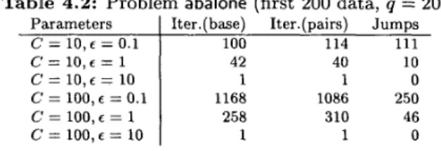
Table 4.2: Problem abalone (first 200 data, q = 20)

Parameters Iter.(base) Iter.(pairs) Jumps

c =

l o , € = 1

c

= l o , € = 10 c' = 100, E = 0.1

c

= 100,e = 1

c

= 100, E = 10 1086 250 1168 258 310

We consider two regression problems abalone (4177 data) and add10 (9792 data) from [l] and [ 5 ] , respec- tively. The RBF kernel is used:

Q . = e-ll.*-5~112/n

23

-

where n is the number of attributes in each data. For these two problems, n is eight and ten, respectively. We use a simple implementation written in MATLAB so only small problems are tested. We consider the first 200 data points of abalone and a d d l 0 . Results are in Tables 4.1 t o 4.4. For each problem we test two different sizes of the working set: q = 1 0 and q =

20. Then in each table we try different E and C . We

did not do any model selections as our purpose is not on the solution quality. We consider E below t o 0 . 1 because the number of support vectors has approached the number of training data. On the other hand, the largest E used is 10 as the number of support vectors has

been close t o zero. For each parameter set, we present the number of iterations by both approaches using base set and pairs of variables, number of support vectors (bounded support vectors), and the number of jumps. If pairs of indices are used, the working set is the union

Table 4.3: Problem add10 (first 200 data, q = 10)

Parameters

c = 1 0 , € = 1 0

c

= 100, E = 0.1 2519 2094 112

c

= 100,E = 1 944 956

c

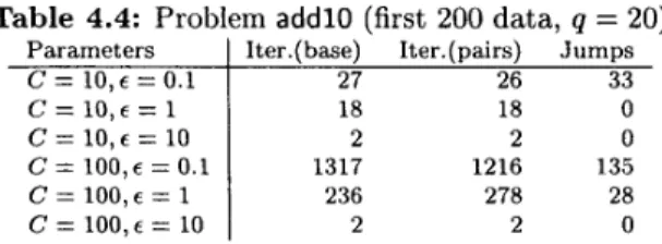
= 100,e = 10

Table 4.4: Problem add10 (first 200 data, q = 20)

Parameters Iter.(base) Iter.(pairs) Jumps

c

= 10, € = 10

c

= loo,€ = 1 236 278 28

c

=

loo,€

= 10 2 2

c

= 100, e = 0.1 1317 1216 135

of two sets: B from (2.7) and its complement B*. We check that before and after solving the sub-problem, how many components of (YB* are changed. Then the total number of such changes are shown in the "Jumps" column.

It can be clearly seen that both approaches have similar number of iterations. In addition, the number of jumps is very small, especially when E is larger. In addition, it can be clearly seen that comparing t o the totally about 1ter.xq components of B* (the size of B* in each iteration may be less than q if B contains pairs; this seldom happens, from Corollary 3.5), the number of components changed is very small.

Acknowledgments

This work was supported in part by the National Sci- ence Council of Taiwan via the grant NSC 89-2213-E- 002- 106.

References

[l] C. L. Blake and C. J . Merz. UCI repository of machine learning databases. Technical report, University of California, Department of Information and Computer Science, Irvine,

CA,

1998. Available at http://www.ics.uci.edu/-mlearn/MLRepository.html

[2] C.-C. Chang and C.-J. Lin. L I B S V M : a library

for support vector machines, 2001. Software available at http://www.csie.ntu.edu.tw/"cjlin/libsvm.

[3] R. Collobert and S. Bengio. SVMTorch: A support vector machine for large-scale regression and classification problems. Journal of Machine Learn- ing Research, pages 143-160, 2001. Available at http://www.idiap.ch/learning/SVMTorch.html.

[4] G. W. Flake and S. Lawrence. Efficient SVM regression training with SMO. Machine Learning, 2001. To appear.

[5] J. Friedman. Multivariate adaptive regression splines. Technical Report No. 102, Laboratory for Com-

putational Statistics, Department of Statistics, Stan- ford University, 1988.

[6] T . Joachims. Making large-scale SVM learning practical. In B. Scholkopf, C. J . C. Burges, and A. J.

Smola, editors, Advances in Kernel Methods

-

Support Vector Learning, Cambridge, MA, 1998. MIT Press. [7] S. Keerthi, S. Shevade, C. Bhattacharyya, and K. Murthy. Improvements to SMO algorithm for SVM regression. Technical Report CD-99-16, Department of Mechanical and Production Engineering, National Uni- versity of Singapore, 1999. To appear in IEEE Trans- actions on Neural Networks.

[SI S. Keerthi, S. Shevade, C. Bhattacharyya, and K. Murthy. Improvements t o Platt's SMO algorithm for SVM classifier design. Neural Computation, 13:637- 649, 2001.

[9] P. Laskov. An improved decomposition algorithm for regression support vector machines. In Workshop o n Support Vector Machines, NIPS99, 1999.

[IO] P. Laskov. An improved decomposition algorithm for regression support vector machines. Machine Learn- ing, 2001. To appear.

[ll] S.-P. Liao, H.-T. Lin, and C.-J. Lin. A note on the decomposition methods for support vector regression. Technical report, Department of Computer Science and Information Engineering, National Taiwan University, 2000.

[12] C.-J. Lin. On the convergence of the decomposi- tion method for support vector machines. I E E E Trans- actions o n Neural Networks, 2001. To appear.

[13] C.-J. Lin. Stopping criteria of decomposition methods for support vector machines: a theoretical jus- tification. Technical report, Department of Computer Science and Information Engineering, National Taiwan University, Taipei, Taiwan, 2001.

[14] J. C. Platt. Fast training of support vector machines using sequential minimal optimization. In B. Scholkopf, C. J. C. Burges, and A. J. Smola, editors, Advances in Kernel Methods

-

Support Vector Learn- ing, Cambridge, MA, 1998. MIT Press.

[15] S. Ruping. mySVM

-

another one of those support vector machines, 2000. Software available at http://www-ai.cs.uni-dortmund.de/SOFTWARE/MYSVM/.

[16] A. J. Smola and B. Scholkopf. A tutorial on sup- port vector regression. Neuro COLT Technical Report TR-1998-030, Royal Holloway College, 1998.

[17] V. Vapnik. Statistical Learning Theory. Wiley, New York, NY, 1998.