多攝影機運動捕捉系統中基於人體模型之姿態估測研究

 

國 立 交 通 大 學

電子工程學系 電子研究所碩士班

碩

士

論

文

多攝影機運動捕捉系統中基於人體模型之姿態

估測研究

Model-Based Pose Estimation for Multi-Camera

Motion Capture System

研 究 生：蕭晴駿

指導教授：王聖智 博士

多攝影機運動捕捉系統中基於人體模型之姿態

估測研究

Model-Based Pose Estimation for Multi-Camera Motion

Capture System

研 究 生：蕭晴駿   Student：Ching-Chun Hsiao

指導教授：王聖智博士 Advisor：Dr. Sheng-Jyh Wang

國 立 交 通 大 學

電子工程學系 電子研究所碩士班

碩 士 論 文

A Thesis

Submitted to Department of Electronics Engineering & Institute of Electronics College of Electrical and Computer Engineering

National Chiao Tung University in partial Fulfillment of the Requirements

for the Degree of Master in

Electronics Engineering July 2008

Hsinchu, Taiwan, Republic of China  

多攝影機運動捕捉系統中基於人體模型之姿態

估測研究

 

研究生：蕭晴駿 指導教授：王聖智 博士

國立交通大學

電子工程學系 電子研究所碩士班

摘要

不論在安全監控、人機互動、電腦動畫或甚至醫學應用上，人物

動作的擷取與分析是個相當重要的議題。在本論文中，我們提出一個

在多攝影機環境下，利用人體模型估測目標人物的姿勢與行為。我們

使用流形嵌入技術中的拉普拉斯特徵映射，將三維人形的幾何形狀忠

實地轉移到另一個容易切割分析的高維度空間，正確地切割出三維人

形的各個部位並且找出三維人形的骨骼架構，以利後續行為分析的動

作。當擷取出三維人形的骨骼架構後，我們利用粒子群體最佳化在高

維度空間中有效地找出最佳姿態估測結果。我們的系統由影像的擷取

至姿態的估測完全自動化，並且不需要在人體上貼附感應物，即可結

合肢體的運動限制和時間軸上的動作流暢限制，估測多種動作。

 

Model-Based Pose Estimation for Multi-Camera

Motion Capture System

Student : Ching-Chun Hsiao Advisor : Dr. Sheng-Jyh Wang

Department of Electronics Engineering, Institute of Electronics

National Chiao Tung University

Abstract

In this thesis, we propose a 3-D human body pose estimation method

using multiple cameras. The reconstructed human body is transformed to

a high dimensional space using our modified Laplacian Eigenmap. In this

eigenspace, the body parts can be segmented more efficiently and easily.

Then, the 3-D skeletons of the human body are extracted to obtain the

kinematic information. Finally, pose estimation is performed by fitting a

prior 3-D model to the extracted skeleton via particle swarm optimization

(PSO). PSO is suitable for the optimization problem with nonlinear cost

functions and doesn’t need too much computational cost. Furthermore,

with our proposed human model, the motion constraints can be easily

combined with the optimization process. Temporal consistency of the

pose estimation results is also achieved by adding temporal constraints

over PSO. Our method can deal with various kinds of motion and has

robust pose estimation results.

誌謝

很感謝王聖智老師從大三到碩二這段期間，給予我們耐心的指導，從專題到論文 研究，不論是訂定題目、研究相關論文和問題的探討與解決，老師總是耐心開導 與指引，從老師身上，學到了許多研究精神和待人接物的道理，也是我們心目中 的模範。也感謝實驗室的學長姐、同學和學弟們，不論是什麼問題和困難，大家 總是能一起分擔、互相幫忙：特別感謝敬群學長，在我研究起步與遇到瓶頸時， 給予很多建議和幫忙，學長也是我們實驗室的活力來源;也感謝奕安、瑞男、庭 瑋和文中，謝謝你們忙碌於實驗室的大小事務，特別是我有這麼快速的電腦可以 拿來實驗模擬，真的很謝謝你們的幫忙！同時也謝謝我的家人，你們是我前進的 動力與支持力，也是我永遠的依偎和寶貝。還要感謝我親愛的好姊妹們，勻珮、 尊宇和婉清，謝謝你們的陪伴和關懷，讓我感受到無敵大溫暖。最後要感謝博凱， 因為你一路走來的支持和幫助，和我一起品嚐研究生活的酸甜苦辣，讓我覺得既 幸福又珍貴，更是我力量的泉源。很謝謝Vision Lab 帶給我的一切，不論是研究 精神的養成和友情的溫暖，畢業的學長姐們也很熱心的協助我找工作，能加入這 個實驗室真的太幸福了！真的很感謝大家！

Contents

Chapter 1. Introduction ... 1

Chapter 2. Backgrounds ... 3

2.1 Motion Capture Systems ... 3

2.1.1 Model-Based Systems ... 4

2.1.1.1 Monocular Motion Capture... 4

2.1.1.2 Multiple View Motion Capture ... 5

2.1.2 Model-Free Systems ... 10

2.2 Manifold Learning ... 13

2.2.1 Manifold Embedding Methods ... 13

2.2.2 Embedding Based Initialization ... 15

Chapter 3. Proposed Method ... 20

3.1 Initialization of Motion Capture ... 21

3.1.1 Images Acquisition... 21

3.1.2 Camera Calibration ... 22

3.1.3 Visual Hull Reconstruction ... 22

3.1.4 Human Body Segmentation ... 30

3.1.4.1 Sunaresan’s Method ... 30

3.1.4.2 Modified Body Parts Segmentation Method... 34

3.1.5 Skeleton Extraction ... 40

3.1.5.1 Sundaresan’s Method ... 40

3.1.5.2 Modified Skeleton Extraction Method ... 41

3.2 PSO Based Pose Estimation... 41

3.2.1 3-D Human Model ... 42

3.2.1.1 Twists and Exponential Products Formulation ... 42

3.2.1.2 3-D Skeleton Model ... 44

3.2.2 PSO Based Pose Estimation ... 49

3.2.2.1 Evaluation Function ... 49

3.2.2.2 Hierarchical PSO Fitting Process ... 51

3.2.2.3 Motion Constraints... 53

3.2.2.4 Fine Tune the Pose Estimation Results ... 54

3.2.2.5 Temporal Consistency ... 55

Chapter 4. Experimental Results ... 57

Chapter 5. Conclusions ... 75

Reference ... 76  

List of Tables

Table 3-1 The notation of the lengths of the body parts ... 45 

Table 3-2 The values of the parameters for the initial configuration ... 46 

Table 3-3 The Hierarchical structure of our fitting process ... 52 

Table 3-4 The motion constraint for each joint ... 54 

List of Figures

Figure 1-1 Depth ambiguity problems exist in monocular approaches[20]... 1 

Figure 2-1 2-D human model examples (a) The 2-D skeleton human model consists of 17 kinematic chains (b) flesh the model in (a) by conical sections[15] ... 4 

Figure 2-2 The pose estimation results in [15] ... 5 

Figure 2-3 The visual hull is constructed by volume intersection [5] ... 6 

Figure 2-4 A look up table is kept to record the voxels which are projected into the same pixel [21] ... 7 

Figure 2-5 3-D articulated human body model used in [13] ... 7 

Figure 2-6 The flow chart of Mikic’s approach [13] ... 8 

Figure 2-7 Pose estimation and visual hull texturing results in [22] ... 8 

Figure 2-8 The pose estimation scheme of [7] : (a) Input images (b) detected foreground (c) reconstructed visual hull (d) extracted medial axis points (e) fitted skeleton model ... 9 

Figure 2-9 Hierarchical fitting process: (a) root position and orientation (b) shoulders and trunk (c) all are fitted [8] ... 9 

Figure 2-10 Pose estimation results from single silhouette [3] ... 10 

Figure 2-11 The flow chart of Elgammal’s method. [4] ... 11 

Figure 2-12 3-D pose estimation results of Elgammal’s method. [4] ... 11 

Figure 2-13 The flow chart of [27] ... 12 

Figure 2-14 Pose estimation results of [27] ... 12 

Figure 2-15 The geodesic distance between two points on the manifold “Swiss roll” is represented by the solid lines. Their Euclidean distance is the dotted line. It is obvious that the geodesic distance is a more reasonable measure to describe the relation between these two marked points [14]. ... 14 

Figure 2-16 Illustration of the three steps of LLE [25]. ... 14 

Figure 2-17 Three manifold embedding results for Swiss roll [2] ... 15  Figure 2-18 The processing flow of [9] : (a) the input sequence from multiple cameras (b) reconstructed volume data (c) transformed volume data in the 3-D embedding space (d) use NSS to obtain skeleton point features (e) project skeleton points back into the normal space to obtain the skeleton curves (f) a sequence of skeleton

curves (g) a normalized kinematic model is estimated from (f) (h) use the

normalized kinematic model to perform pose estimation ... 16 

Figure 2-19 The segmentation process of [10]: (a) input 3-D voxel data (b) LLE transformation results and branch termination detection (c) segmentation using k-wise clustering in the embedded space (d) segmentation results in the normal space ... 17 

Figure 2-20 Clustering seeds are propagated along time to ensure temporal consistency [10] ... 17 

Figure 2-21 Embedding results using different manifold learning techniques [6] ... 18 

Figure 2-22 Pose estimation process of [6]: (a) input images from multiple cameras (b) 3-D voxel data acquired by space carving (c) transform the 3-D data using LE and segment it using spline fitting (d) project the segmented chains back into the normal space (e) skeleton extraction (f) top-down pose estimation ... 19 

Figure 3-1 The block diagram of the proposed system ... 20 

Figure 3-3 Visual hull reconstruction using volume intersection ... 22 

Figure 3-4 The setup of four cameras in our laboratory ... 25 

Figure 3-5 The circular configuration of the OVVV virtual cameras: eight cameras are separated by the angle of 45° ... 25 

Figure 3-6 (a) four captured images in our laboratory (b) reconstructed visual hull . 26  Figure 3-7 (a)(b) eight captured images in the OVVV simulation environment (c) reconstructed visual hull ... 27 

Figure 3-8 (a)(b) eight capture images from Camera1~Camera8. (c) reconstructed visual hull from eight cameras. (d) reconstructed visual hull from Camera1~Camera4. (e) the superposition of (c) over (d), where the green parts are the visual hull of (c) while the blue parts are that of (d). the yellow parts represent the overlap of (c) and (d) ... 28 

Figure 3-9 The formation of ghost legs: for clearness, the cone-like volume started from camera centers are simplified using trapezoid solid. The intersection is represented as red and black hexagons. Red hexagons are real visual hull while black ones are artifacts. Two circles marked “L” and “R” represented left leg and right leg of a specific person. ... 29 

Figure 3-10 The body parts segmentation process of Sundaresan’s method (a) one of the eight captured images (b) reconstructed visual hull (c)(d) the Laplacian Eigenmap transformation result: dimension1~dimension6 (e) spline initialization for the green branch in dimension1~3 (f) spline propagation and then termination for the green branch in dimension1~3 (g) six segmented braches: black points represent the unfitted ones (h) transform the segmentation results back to the normal space. Most of the nodes in the torso part are unfitted. ... 32 

Figure 3-11 (a) test image (b) the result of Laplacian Eigenmap transformation. (c) the segmentation result in the eigenspace (d) illustration of the failed spline fitting for the thick branch. Here, the cyan branch is zoomed in for clearer illustration. The cross and the two dashed lines represent the starting point of the cyan branch and

the first two principal components, respectively. ... 33 

Figure 3-13 The color weight curve... 36 

Figure 3-15 Comparison between Sundaresan’s segmentation method and ours (a) one of the eight input images (b) the color representation for the segmentation results (c) the segmentation result in the first three dimension of the eigenspace using original LE (d) the segmentation result in the last three dimension of the eigenspace using original LE (e) the segmentation result in the normal space using original LE (f) the segmentation result in the first three dimension of the eigenspace based on our modified method (g) the segmentation result in the last three dimension of the eigenspace based on our modified method (h) the segmentation result in the normal space using our modified method ... 39 

Figure 3-16 The skeleton extraction result using proposed method (a) one of the eight input images (b) spline fitting and site value calculation in the 1-D eigenspace (c) the extracted skeleton ... 41 

Figure 3-17 An object rotates θ radians about a fixed axis ω ... 42 

Figure 3-18 The rigid body transformation of an open kinematic chain ... 44 

Figure 3-19 3-D human skeleton model ... 44 

Figure 3-20 The weakness of Mikic’s method ... 47 

Figure 3-21 For the dark blue skeleton, we sample 6 nodes and use them to calculate the fitting error respect to the 6 different body parts (head, torso, arms, and legs) in the human model separately. 6 points are also marked from each body part segment. ... 50 

Figure 3-22 The mechanism that ensures the temporal consistency ... 55 

Figure 4-1 The second setup of eight cameras for oursynthetical environment ... 58 

Figure 4-2 The pose estimation results of s1. The first two rows are the 8 different frames captured by the eight different cameras at a specific time instant. The 3rd and 4th rows are the reconstructed visual hulls. The 5th and 6th rows are the segmented visual hulls. The extracted skeletons are plotted in the 7th and 8th rows. The fitting results are shown in the 9th and 10th rows. The last two rows are the pose estimation results. ... 60 

Figure 4-3 The pose estimation results of sequence s2. The 1st to 4th rows are the input images from one of the eight cameras. The 5th to 8th rows show the extracted skeleton and the fitting results. Pose estimation results are shown in the last four rows. ... 62 

Figure 4-4 The pose estimation results of sequence s3. The first four rows are the input

images from one of the eight cameras. The 5th to 8th rows show the skeleton

extraction and the model fitting results. The last four rows are the results of pose estimation ... 64  Figure 4-5 The pose estimation results of sequence s4. The first three rows are the input images from one of the eight cameras. The extracted skeleton and its model fitting

results are shown in the 4th to 6th rows. The last three rows show the pose

estimation results. ... 66 

Figure 4-6 The pose estimation results of sequence s5. The 1st to 3rd rows show the input

images from one of the eight cameras at 12 different time instants. The 4th to 6th

rows are the extracted skeleton and the fitting results. The last three rows show the pose estimation results. ... 67  Figure 4-7 The pose estimation results of sequence s6. Input images from one of the

eight cameras are shown in the first four rows. 5th to 8th rows are the results of the extracted skeleton and model-fitting. The last four rows show the results of pose estimation. ... 69  Figure 4-8 The pose estimation results of s7. The first three rows are the input images

from one of the eight cameras. The 4th to 6th rows show the extracted skeleton and

model-fitting results. The pose estimation results are shown in the last three rows.

... 71 

Figure 4-9 The pose estimation results of sequence s8. The 1st to 3rd rows show the input

images from one of the eight cameras. The 4th to 6th rows are the extracted skeleton

and model-fitting results. The pose estimation results are shown in the last three rows. ... 72  Figure 4-10 The pose estimation results of sequence s9. The first four rows are the input

images from one of the eight cameras. The next four rows show the extracted skeleton and the fitting results. The last four rows are the pose estimation results.

Chapter 1.

Introduction

Human motion capture is to estimate the configuration of human body parts using inputs from one or more video streams. It has gained in popularity among surveillance, human-machine interaction, computer animation and medical applications. Typically, a motion capture system can be classified into marker-based or markerless. Marker-based motion capture systems require the human body be equipped with markers. However, the use of markers is very cumbersome and may restrict the freedom in observation. Furthermore, this approach is expensive and it is hard to align kinematic motion to marker data. Recently, there have been two main approaches, monocular approach and multi-camera approach, for markerless motion capture system. The advantages of monocular approach are simple hardware setup and lower cost. However, as shown in Figure 1-1, there exist depth ambiguities when only one silhouette is available. Hence, multi-camera approaches, which reconstruct 3-D human bodies from a set of silhouettes, are preferred to offer more information for motion capture systems. With more view angles we can alleviate the occlusion problem and make the motion capture system more robust.

Figure 1-1 Depth ambiguity problems exist in monocular approaches[20]

In this thesis, we propose a markerless motion capture system equipped with multiple cameras. First, a 3-D human body represented by voxels is reconstructed from multiple video streams. A modified Laplacian Eigenmap algorithm is used to transform the 3-D voxel data into a high dimensional space. With this manifold embedding method, different body parts are mapped into discriminative branches and can be easily segmented. Unlike other approaches, this approach relieves the

dependence on human model and the training database. After the segmentation of body parts, skeletons are extracted to describe the kinematic motion of the human body. Human shapes are usually deformed while skeletons can encode most of the motion information. As the skeletons are extracted from the 3-D human bodies, we use the particle swarm optimization (PSO) technique to deal with the pose estimation problem. The experimental results show that our system can handle various kinds of poses and can ensure temporal consistency and motion constraints.

This thesis is organized as follows. In Chapter2, we introduce the background of motion capture systems. In Chapter3, we discuss the properties of the Laplacian Eigenmap and the proposed pose estimation approach. Experimental results are shown in Chapter4. Finally, we will make a brief conclusion in Chapter5.

Chapter 2.

Backgrounds

In this chapter, we will introduce a few motion capture approaches developed in recent years. Firstly, a brief introduction to motion capture and its functional taxonomy are discussed in Chapter 2.1. Since we’ll focus on markerless motion capture systems equipped with multiple cameras, related algorithms are also mentioned in Section 2.2.

2.1

Motion Capture Systems

Some popular motion capture algorithms are to be reviewed in this section. Since systems with markers are costly and ineffective, we mainly discuss markerless motion capture systems, which have drawn much attention in recent years. According to the survey in [26], we can decompose markerless approaches into several submodules based on the following functional taxonomy:

y Initialization: the initialization of motion capture systems tends to acquire some prior knowledge for pose analysis. The prior knowledge may include kinematic structure, 3-D human shape, and so on.

y Tracking: this process typically includes foreground detection and continuous target tracking in the video.

y Pose estimation: given some prior knowledge obtained in the initialization step, this process tries to estimate the posture of a specific person.

y Recognition: this process identifies the activities or behaviors of the target person, such as running, walking, and so on.

In the proposed motion capture system, we mainly focus on the initialization module and the pose estimation module. The module of initialization aims to obtain reliable prior knowledge for pose estimation and recognition. Due to error propagation, incorrect prior knowledge may lead to wrong pose estimation. In the following discussion, we will focus on a few algorithms which are related to initialization and pose estimation.

In general, markerless motion capture systems can be classified into model based systems and model free systems, depending on whether a prior human model is used in the system. In the following sections, we will introduce several popular motion capture systems in each of these two categories.

2.1.1 Model-Based Systems

Model based systems use an explicit model to capture the motion of a specific person. Depending on whether the system is monocular or multi-view, the model can be either 2-D or 3-D. In the following subsections, we will briefly introduce model-based systems based on these two system types.

2.1.1.1

Monocular Motion Capture

Monocular motion capture systems only use one camera and deal with the problems in the 2-D image planes. For 2-D model-based motion capture systems, contour human models, stick models, and cardboard models are commonly used.

Figure 2-1 2-D human model examples (a) The 2-D skeleton human model consists of 17 kinematic chains (b) flesh the model in (a) by conical sections[15]

Deutscher [15] modified the particle filtering algorithm to estimate the posture in the 2-D image plane. Given foreground silhouettes, 2-D human models as shown in Figure 2-1 are used to fit the detected human bodies. In this approach, human models are composed of 17 chains connected by joints. Each joint has its degree of freedom (DOF) and the whole model adds up to 29 DOF. Pose estimation is performed by fitting the human model to the foreground silhouettes. The fitting result, as illustrated in Figure 2-1 (b), describes the posture of the person. However, the searching space of this approach is too large due to the high DOF. Even though the particle filter has been a useful tool in data fitting, it may get trapped in a local maximum and does require lots of computation in a search space of high dimensionality. In [15], the anneal particle filtering is adopted to effectively find the global maximum. However,

depth ambiguities still exist and the processing speed is far too slow (about 1 hour for a 5-second footage).

Figure 2-2 The pose estimation results in [15]

2.1.1.2

Multiple View Motion Capture

Estimating posture from 2-D images only is rather difficult. This is because the self occlusion problem and the depth ambiguity problem cannot be properly handled. In order to obtain more robust motion capture results, 3-D data are more preferable. In [5], the reconstruction of a “visual hull” based on images from multiple cameras is introduced. A visual hull is defined as the 3-D shape formed by the intersection of visual cones projected from the 2-D silhouettes, as illustrated in Figure 2-3 [5]. The

visual hull of an object can be thought to be a close approximation of the object based on the observations from different viewpoints.

Figure 2-3 The visual hull is constructed by volume intersection [5]

The visual hull can be represented by voxels and several algorithms have been developed to construct the visual hull based on a set of silhouette. In practice, we don’t actually compute the visual cones and their intersection. It’s computationally costly and difficult to find their intersection parts. Instead, when implementing the visual hull reconstruction algorithm, voxels are back projected to the image planes to check whether their projections fall into the region of the foreground silhouettes. Then, the silhouettes on multiple cameras vote to decide whether a voxel belongs to the visual hull. Szeliski [24] proposed an octree representation of the voxel space where the resolution of voxels is variable according to their projections on the image planes. It can reconstruct a visual hull from coarse resolution to fine resolution. However, this approach is sensitive to the hypothesis of visibility. Kehl [22] introduced a fast visual hull construction method. A voxel look-up table is built to record the projection position in each image plane for all the voxels. To speed up the process while maintaining the high-resolution voxels, the projection is approximated by a cross patch. As shown in Figure 2-4, Voxels 7, 12 and 15 project to the same position in the image plane. Hence, they are recorded in the look-up table of that pixel. Once that pixel is labeled as “foreground”, these voxels may belong to the visual hull.

Figure 2-4 A look up table is kept to record the voxels which are projected into the same pixel [21]

To model the 3-D shape of the visual hull, Mikic [13] adopted a twist framework that has been used to model the kinematic chains for robots. Sixteen rotation axes and five kinematic chains of the body joints are formulated using twists and product of exponentials. Based on a torso-centered coordinate system, the rotation and shift of the body parts can be easily manipulated. Given voxel data reconstructed from 6 calibrated and synchronized cameras, pose estimation is performed by first doing template fitting and then using Bayesian network for refinement. However, the initialization of this approach is based on template fitting, which cannot deal with self occlusion. Moreover, this approach requires that the target person be dressed in tight clothes.

Figure 2-6 The flow chart of Mikic’s approach [13]

Kehl [22] proposed a stochastic meta descent (SMD) optimization method to fit the body model to the visual hull. SMD is the generalization of gradient descent. It adapts its local step size to offer more rapid convergence and uses stochastic sampling to avoid being trapped in a local minimum.

Figure 2-7 Pose estimation and visual hull texturing results in [22]

Instead of using shape models, Menier [7] adapted skeleton models to fit medial axis points extracted from visual hulls. This approach reduces the dependency on the dimension of human body. These 3-D medial axis points represent the observed skeleton data. A generic skeleton model is then fitted with the observed skeleton data based on a maximum a posteriori (MAP) estimation. The pose estimation of the first frame is based on the fitting process, while non parametric belief propagation is used to predict the pose in the following frames.

Figure 2-8 The pose estimation scheme of [7] : (a) Input images (b) detected foreground (c) reconstructed visual hull (d) extracted medial axis points (e) fitted skeleton model

Due to the high dimensionality of the search space and the complexity of the fitness evaluation function, some researchers have adopted particle swarm optimization (PSO) method to perform pose estimation. PSO [16] is an optimization technique that simulates the social behaviors of animals. Given a fitness function and a communication network, particles gradually move to the best position according to the self experience and the information obtained from their neighbors. Robertson [8] applied PSO to perform skeleton model fitting in a conference room environment, where the pose estimation is required only for the upper body. PSO is chosen for its ability to deal with nonlinear and non-convex optimization problems. Hierarchical and parallel PSO fitting is proved to be robust and computationally inexpensive.

(a) (b) (c) Figure 2-9 Hierarchical fitting process: (a) root position and orientation (b) shoulders and

trunk (c) all are fitted [8]

Model based motion capture systems use a prior model to reduce the search space and hence have less complexity. Moreover, they usually assume tight fitting clothes and the initialization of the human models has great influence on the accuracy of pose estimation. Since template fitting-based initialization cannot well handle self occlusion, embedding-based initialization has drawn much attention recently. In Section 2.2, we will introduce a few popular manifold embedding methods and explain how they are applied to initialize the motion capture systems. These

embedding-based methods may produce robust human body labeling results and make the initialization process less sensitive to human poses and human models. In this thesis, we will also propose a pose estimation method that adopts embedding-based initialization.

2.1.2 Model-Free Systems

Model-free approaches don’t have an explicit model. For most of this kind of motion capture systems, pose estimation is made by comparing the observed data with the database or by a pre-learnt mapping relation between the input images from the training data and their pose estimation results.

Agarwal [3] proposed a learning-based pose estimation for monocular motion capture systems. A shape descriptor is extracted from silhouettes to overcome the foreground segmentation errors. A database is used to train the relevance vector machine (RVM) and decisions are made after machine learning. Without the need of human models and initialization process, a 3-D pose can be estimated from a single silhouette.

Figure 2-10 Pose estimation results from single silhouette [3]

Elgammal [4] applied the manifold learning methods to pose estimation. For the learning step, the mapping between silhouettes and 3-D poses are constructed using locally linear embedding (LLE), which is a nonlinear manifold embedding method. Then, pose estimation is done based on the manifold embedding results. That is, given detected silhouettes, its 3-D pose estimation is obtained from the mapping relation learned by LLE.

Figure 2-11 The flow chart of Elgammal’s method. [4]

Figure 2-12 3-D pose estimation results of Elgammal’s method. [4]

Sagawa [27] proposed an example-based approach to perform pose estimation. For each frame, the feature vector is first extracted from the reconstructed 3-D voxel data and then compared with the database. The evaluation process is further improved by a graphical model of motion that ensures the temporal consistency.

Figure 2-13 The flow chart of [27]

Figure 2-14 Pose estimation results of [27]

Model-free systems have the advantages of lower computational cost and can avoid large search space and nonlinear optimization. However, the performance of a model-free motion capture system greatly depends on the database. If the database is not diverse enough, the decision may be biased and may result in inaccurate pose estimation.

2.2

Manifold Learning

As mentioned earlier, model based motion capture systems have the advantages of complexity reduction and robustness. However, a good initialization is required to ensure that the system commences with a good body parts labeling and initial guess. Template fitting cannot deal with self occlusion while direct fitting human models to 3-D data results in high dimensionality of the search space. More reliable initialization approaches based on manifold learning have been proposed recently. In manifold learning, the intrinsic geometric properties are preserved after mapping the 3-D data to another space. Furthermore, this method makes the body parts labeling much easier and reliable. In the following sections, we will firstly introduce some manifold learning methods and then discuss how they are applied to motion capture.

2.2.1 Manifold Embedding Methods

Manifolds are defined as a topological space which is locally Euclidean [1]. Manifold embedding is a topic about how to find a transformed space for the manifold that preserves the connectivity and algebraic properties. Usually, manifolds are the data lying in the high dimensional space and the transformation helps reduce the dimensionality. Therefore, manifold embedding is a useful tool for dimension reduction. There have been many manifold embedding methods which can be classified into linear approaches and nonlinear ones. Linear manifold embedding methods such as principal component analysis (PCA) and multidimensional scaling (MDS) assume the data is a linear function of the features. This assumption isn’t general and cannot deal with nonlinear cases. More generalized nonlinear approaches have been proposed since 2000. ISOMAP, locally linear embedding (LLE) and Laplacian Eigenmap (LE) are graph-based methods among the popular manifold embedding methods.

In these graph-based methods, graph models are used to approximate the structure of the manifold. A graph-based manifold embedding method typically have three basic steps:

1. Find the k nearest neighbors for each node to construct the graph. 2. Local properties in the neighborhood of each node are estimated.

3. Embed the graph globally to another space that preserves the local properties estimated in Step2.

the geodesic distances. Geodesic distance is a better measure than Euclidean distance for manifolds. However, the Euclidean distance is much easier to calculate. Hence, the geodesic distance between any two points is approximated by a chain of short paths, whose distance is calculated using Euclidean distance.

Figure 2-15 The geodesic distance between two points on the manifold “Swiss roll” is represented by the solid lines. Their Euclidean distance is the dotted line. It is obvious that the geodesic distance is a more reasonable measure to describe the relation between these two marked points [14].

Locally linear embedding (LLE) [25] assumes that manifolds are linear when viewed locally. For each node, the k nearest neighbors are selected. Then the LLE method reconstructs each node based on the linear combination of their k neighbors. The geometric properties are preserved by choosing the linear weights of these neighbors to minimize the reconstruction error.

Figure 2-16 Illustration of the three steps of LLE [25].

On the other hand, Laplacian Eigenmap (LE) [18] uses graphs and Laplacian of the graphs to approximate the manifold structure and the Laplacian Beltrami operator,

respectively. Laplacian Beltrami operator is the extension of the second-order differential operator, Laplacian, and is defined on manifolds as well as on surfaces. It can be shown that the eigenfunctions of the Laplacian Beltrami operator can well preserves the intrinsic geometric properties. Similarly, the eigenvectors of the Laplacian of the graph provide the appropriate embedding as well. Instead of preserving the geodesic distances, LE attempts to make the adjacent nodes in the normal space close to each other in the embedding space. By this approach, the intrinsic geometric properties can be easily preserved.

(a) Swiss roll (b) Intrinsic structure of the swiss roll

(c) ISOMAP (d) LLE (e) LE

Figure 2-17 Three manifold embedding results for Swiss roll [2]

2.2.2 Embedding Based Initialization

Since manifold embedding methods can preserve geometric properties, some embedding based systems have recently been proposed for motion capture. These manifold embedding based methods are independent of human models and are hence less restricted. Moreover, the embedding spaces possess some useful properties that make the initialization process simpler and more robust.

Chu [9] applied ISOMAP to motion capture systems. The fact that a prior human model is no longer needed makes the initialization process less restricted and more reliable. For each frame, skeleton points are extracted using ISOMAP. Finally, a kinematic model is fitted to each frame to perform pose estimation. ISOMAP can transform the 3-D volume data into a pose-independent space, which preserves the intrinsic geometric structure. Next, the nonlinear spherical shells (NSS) method is

used to perform partitioning and clustering in the embedding space to obtain tree-structured principal curves. Finally, the curves are projected back to the normal space and the skeleton point features are extracted. Based on the sequence of the skeleton curves, a normalized kinematic model can be constructed. Pose estimation is done by applying this kinematic model to all frames.

Figure 2-18 The processing flow of [9] : (a) the input sequence from multiple cameras (b) reconstructed volume data (c) transformed volume data in the 3-D embedding space (d) use NSS to obtain skeleton point features (e) project skeleton points back into the normal space to obtain the skeleton curves (f) a sequence of skeleton curves (g) a normalized kinematic model is estimated from (f) (h) use the normalized kinematic model to perform pose estimation

LLE is also applied to human motion capture. Cuzzolin [10] proposed a robust body parts labeling method along the temporal axis based on LLE. Temporal information is added to help segment the body parts in a consistent way. Unlike ISOMAP, LLE can enhance the separation of different body parts, which make the body parts segmentation much easier. Moreover, ISOMAP is computationally

expensive. For these reasons, 3-D voxel data is transformed to a 3-D embedding space via LLE. After transformation, the segmentation is done by k-wise clustering. The clustering seeds are propagated through time. The clusters also merge or split according to the topology changes to ensure temporal consistency.

(a) (b) (c) (d) Figure 2-19 The segmentation process of [10]: (a) input 3-D voxel data (b) LLE

transformation results and branch termination detection (c) segmentation using k-wise clustering in the embedded space (d) segmentation results in the normal space

In [6], Sundaresan proposed a segmentation approach for pose estimation based on Laplacian Eigenmap. Unlike ISOMAP, LE tries to preserve the geometric structure instead of geodesic distances. In this approach, different branches in the normal space, such as separated body parts, are transformed into distinguishable smooth curves in the embedding space. Compared with other popular manifold learning methods, only LE and Diffusion map have this special property, as shown in Figure 2-21. This property makes the segmentation of 3-D human body a lot easier. Moreover, since Diffusion map is only a variation of LE, LE is chosen in this thesis for its low computational cost.

(a) Test image

(b) LE (c) ISOMAP (d) MDS (e) LLE (f) Diffusion map Figure 2-21 Embedding results using different manifold learning techniques [6]

LE also has two extra important properties:

y Different branches in the normal space are mapped into different curves in the eigenspace. The higher the dimensionality of the eigenspace is, the better the discriminative capability is.

y Braches with the length-over-width ratio greater than 2 can be mapped to smooth curves. Moreover, due to the preservation of geometric relationship, one can infer the position of the node in the branch by its position in the curve.

To sum up, n chains whose lengths are twice longer than their widths can be mapped into n discriminative smooth curves in the eigenspace whose dimension is

between n-1 and 2n.

After transformation, nodes in the curves can be segmented using spline fitting. In the eigenspace, each node has its “site value” which represents its position along the chain. The site values are used to extract the skeletons from the visual hull. A generic human model is then fitted to the skeleton data in order to estimate the posture.

(a) (b) (c) (d) (e) (f) Figure 2-22 Pose estimation process of [6]: (a) input images from multiple cameras (b) 3-D voxel data acquired by space carving (c) transform the 3-D data using LE and segment it using spline fitting (d) project the segmented chains back into the normal space (e) skeleton extraction (f) top-down pose estimation

     

Chapter 3.

Proposed Method

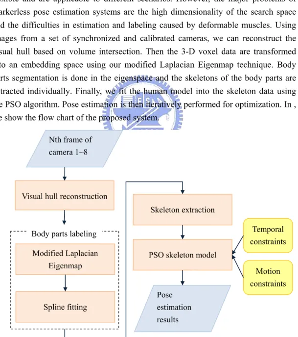
In this thesis, we proposed an efficient initialization process and a robust markerless pose estimation system. The goal of pose estimation is to capture the motion of a specific person. The motion of the articulated body parts is described using some parameters of a generic human model. The motion capture technique has been widely applied to different areas, such as surveillance, computer animation and biomechanical engineering. As mentioned earlier, markerless systems are more flexible and are applicable to different scenarios. However, the major problems of markerless pose estimation systems are the high dimensionality of the search space and the difficulties in estimation and labeling caused by deformable muscles. Using images from a set of synchronized and calibrated cameras, we can reconstruct the visual hull based on volume intersection. Then the 3-D voxel data are transformed into an embedding space using our modified Laplacian Eigenmap technique. Body parts segmentation is done in the eigenspace and the skeletons of the body parts are extracted individually. Finally, we fit the human model into the skeleton data using the PSO algorithm. Pose estimation is then iteratively performed for optimization. In , we show the flow chart of the proposed system.

Nth frame of camera 1~8

Visual hull reconstruction

Modified Laplacian Eigenmap

Spline fitting

Skeleton extraction

PSO skeleton model

Pose estimation results

Body parts labeling Temporal constraints

Motion constraints

We have conducted our experiment in both the synthesized world and the real world environment. For video synthesis, the ObjectVideo Virtual Video (OVVV) [11] is used to simulate different kinds of the camera setup. For the real world environment, four cameras mounted on the ceiling of our laboratory are used. We will discuss these two different environments and explain why we choose OVVV as our simulation tool.

3.1

Initialization of Motion Capture

The initialization of our motion capture systems includes image acquisition, camera calibration, visual hull reconstruction, human body parts segmentation, and skeleton extraction. We will discuss the initialization of our pose estimation system in the following sections.

3.1.1 Images Acquisition

Images are acquired in both the virtual world and the real world. As mentioned earlier, OVVV is our simulation tool for different camera setups. OVVV is developed by ObjectVideo and is based on the game engine offered by “Half Life2.” The architecture of OVVV is shown in Figure 3-2. The virtual cameras can be set up independently with different locations, PTZ parameters, fields of view, frame dimensions and frame rates. After setting up the cameras, virtual video can be rendered and simulated for various kinds of scenarios. With the help of OVVV, the experimental scenarios can be easily repeated and rearranged. This saves a lot of time and cost. On the other hand, for the real world environment, the sequences are acquired by four synchronized cameras mounted in the ceiling of our laboratory. The configuration of these cameras will be discussed later.

3.1.2 Camera Calibration

Camera calibration provides the internal and external parameters of cameras. For the OVVV system, we can obtain these parameters directly from the ground truth. For the real environment, on the other hand, we choose [12] as our calibration tool. Chen has developed an efficient and robust technique for multiple camera calibration. With only two sheets of A4 paper, we can easily obtain the external parameters of four cameras. Once we have acquired the calibration data of multiple cameras in an offline manner, the visual hull can be reconstructed using the volume intersection method.

3.1.3 Visual Hull Reconstruction

Through background subtraction, we can obtain the foreground silhouette of the object in each camera. Visual hull reconstruction is then performed by the volume intersection technique. For the silhouette of each camera, the lines connected the camera center and a silhouette point forms a cone-like area. The intersection of these areas is the 3-D approximation of the target person.

In practice, we project each voxel to the image planes. If the projection falls inside one of the silhouettes, it gets one vote. A voxel is classified as “foreground” if the number of votes exceeds some predefined threshold. The higher the threshold is, the smaller the false alarm rate is. However, the probability of detection may also get decreased when we raise the threshold. Basically, this approach is more effective and is less computationally expensive than the direct implementation of the volume intersection method.

For the OVVV system, back-projections of voxels are evaluated using the calibration ground truth for each camera. Given the rotation angles (θ θ θ_x, , _{y z}), the position (X, Y, Z) and the FOV (field of view) of each camera, the projection of voxels can be calculated as follows:

Rotation matrix: 1 0 0 0 0 cos( ) sin( ) 0 0 sin( ) cos( ) 0 0 0 0 1 x x x x x R θ θ θ θ ⎡ ⎤ ⎢ _{− − −} ⎥ ⎢ ⎥ = ⎢ − − ⎥ ⎢ ⎥ ⎣ ⎦ Eq. 3-1 cos( ) 0 sin( ) 0 0 1 0 0 sin( ) 0 cos( ) 0 0 0 0 1 y y y y y R θ θ θ θ − − ⎡ ⎤ ⎢ ⎥ ⎢ ⎥ = ⎢− − − ⎥ ⎢ ⎥ ⎣ ⎦ Eq. 3-2 cos( ) sin( ) 0 0 sin( ) cos( ) 0 0 0 0 1 0 0 0 0 1 z z z z z R θ θ θ θ − − − ⎡ ⎤ ⎢ _{− −} ⎥ ⎢ ⎥ = ⎢ ⎥ ⎢ ⎥ ⎣ ⎦ Eq. 3-3 Translation matrix: 1 0 0 0 1 0 0 0 1 0 0 0 1 X Y T Z − ⎡ ⎤ ⎢ ₋ ⎥ ⎢ ⎥ = ⎢ − ⎥ ⎢ ⎥ ⎣ ⎦ Eq. 3-4

Camera calibration matrix:

0 0 0 0 0 0 1 0 0 0 fov C fov ⎡ ⎤ ⎢ ⎥ = ⎢ ⎥ ⎢ ⎥ ⎣ ⎦ Eq. 3-5 Projection matrix: * _x* _y* _z* Pj C R R= R T Eq. 3-6

The back projection of a voxel p: (bp vector)

[

1 2 3

]

1 3 1 2 3 2 * _ 2 _ 2 T

imP imP imP Pj p

imP imP img width bp

imP imP img length bp = − ⎡ ⎤ ⎡ ⎤ = ⎢ ⎥ ⎢ ⎥ ₋ ⎣ ⎦ ⎣ ⎦ Eq. 3-7

For the OVVV system, the calibration of multiple cameras refers to the same world coordinate. On the other hand, the four real cameras mounted in the ceiling of our laboratory are calibrated using Chen's method, which aligns all cameras’ coordinates to one of the cameras’ [12]. After calibration, the visual hull can be reconstructed in a similar way. The accuracy of the visual hull depends on several factors as listed below:

y The resolution of the voxels

y The accuracy of the calibration result

y The number and the configuration of cameras y The synchronization among multiple cameras y Foreground detection results

For these two experimental environments, we use 30mm×30mm×30mm voxels to compromise between computational cost and resolution. The calibration and synchronization is fairly accurate for the OVVV environment, since the data actually comes from the ground truth. In comparison, in the real-world environment, the back projections of voxels may deviate around four pixels, which are pretty acceptable. Besides, the background subtraction is used to detect foreground. A more precise background modeling technique based on the mean-shift algorithm is adapted to achieve robust results [19]. The major differences between the OVVV synthetical environment and our laboratory environment are the number of cameras and the configurations of cameras. In the real-world environment, four PTZ cameras are fixed in the ceiling, as shown in Figure 3-4. As for the OVVV environment, we can modify the number of cameras and setup of cameras to enhance the accuracy of the visual hull. Mündermann [17] suggested that the number of cameras should be more than 7 to reduce the artifacts in the visual hull. Four cameras aren’t enough to provide reliable visual hull. Artifacts, such as ghost legs, will impair the results of body parts labeling and pose estimation. To understand how the number of cameras influences the reconstruction of visual hulls, we use OVVV to simulate the environment with eight cameras. As shown in Figure 3-5, the configuration of virtual cameras is circular, with equal height and the cameras are separated by 45 degrees. There are still many different setups for eight cameras. According to [17], the configuration with one camera above the target person and the others equally separated and surrounding the

human body circularly will obtain the most accurate visual hull. To observe the artifacts of the visual hull, we first use the camera configuration shown in Figure 3-5. As for our experimental environment, most of our sequences are captured under the configuration suggested by [17] to alleviate the problem of artifacts.

Figure 3-4 The setup of four cameras in our laboratory

 

Figure 3-5 The circular configuration of the OVVV virtual cameras: eight cameras are separated by the angle of 45°

1.8 m 3.0 m 7 2 ₆ 4 8 3 5 1 3 2.17 m 2.17 m 5.00 m 3.68 m 2 4 1

(a)

(b)

(a) (b)

(c)

Figure 3-7 (a)(b) eight captured images in the OVVV simulation environment (c) reconstructed visual hull

In Figure 3-6, we can see that the visual hull reconstructed in our laboratory has “ghost leg” and lots of artifacts around the arms. The serious artifact problem may result in inaccurate body parts labeling and poor pose estimation. For example, we don’t know whether a leg is real or just is an artifact. On the other hand, the visual hull reconstructed in the OVVV is more accurate. To demonstrate the artifacts in visual hulls, we use OVVV to simulate two different environments with eight and four cameras separately. The 8-camera environment is just like the figure shown in Figure 3-5, while the 4-camera environment is an environment with four of the eight cameras in Figure 3-5.

(a) (b)

(c) (d)

(e)

Figure 3-8 (a)(b) eight capture images from Camera1~Camera8. (c) reconstructed visual hull from eight cameras. (d) reconstructed visual hull from Camera1~Camera4. (e) the superposition of (c) over (d), where the green parts are the visual hull of (c) while the blue parts are that of (d). the yellow parts represent the overlap of (c) and (d)

4 cameras 8 cameras intersection

For the case of four cameras, four apparent legs appear in the visual hull. Compared with that reconstructed from eight cameras, there are also some artifacts around the chest and the back. The formation of ghost legs can be easily illustrated in Figure 3-9. Due to insufficient number of cameras, ghost legs appear inside the intersection of the cone-like volumes. If we back-project the voxels of the four legs into the image planes, they all fall inside the silhouettes. Hence, it’s difficult to identify which two legs are actually artifacts.

Figure 3-9 The formation of ghost legs: for clearness, the cone-like volume started from camera centers are simplified using trapezoid solid. The intersection is represented as red and black hexagons. Red hexagons are real visual hull while black ones are artifacts. Two circles marked “L” and “R” represented left leg and right leg of a specific person.

Serious artifacts, such as ghost legs, will result in inaccurate body parts segmentation. Especially when the calibration isn’t so accurate and the foreground detection results have false positive or false negative, it is hard to remove these artifacts. In order to avoid serious artifacts in visual hull reconstruction, we choose OVVV as our simulation tool to acquire reliable visual hull from eight virtual cameras. C3  C1  C2  C4  R L Top view

3.1.4 Human Body Segmentation

If we can segment each body parts separately, it will help pose estimation a lot. The search space is reduced and we can infer the posture based on the segmented body parts. Among recent research works, the embedding-based methods have the advantage of no model dependency and are robustness for various kinds of stature. These methods apply manifold embedding techniques to transform the original 3-D voxel data to another embedded space. Having preserved the intrinsic properties of the visual hull, the use of transformation makes it much easier to perform human body labeling.

3.1.4.1

Sunaresan’s Method

In [6], Sundaresan has compared Laplacian Eigenmap with other popular manifold embedding methods. The Laplacian Eigenmap method possesses the capability of transforming a 3-D long branch into a smooth curve. After applying Laplacian Eigenmap, the segmentation of human body parts can be easily performed by applying spline fitting over the smooth curves. In Sundaresan’s algorithm, the process of body part segmentation can be summarized as follows.

A. Laplacian Eigenmap Transformation

The first step of the Sundaresan’s algorithm is to transform the visual hull into data in a six dimensional eigenspace. A graph G is constructed to record the relationship among voxels of the visual hull. For each voxel vi in the visual hull, this approach checks the 6-adjacent neighbors of vi. If any of the neighbors, say vj, also belongs to the foreground voxels, then vi and vj are connected by an edge. The eigenvectors of the Laplacian of the graph corresponding to the six smallest nonzero eigenvalues are selected as the basis of the transformation map. In this step, each voxel vi in the visual hull is transformed to a 6-D vector ui.

B. Segmentation in the eigenspace

In the LE transformation, different body parts are transformed into separated smooth branches. The segmentation of body parts is then performed using a spline fitting in the eigenspace. The use of spline fitting segments these branches into individual curves, with each curve labeling a body part in the normal space. The following paragraphs explain three major steps in spline fitting.

B-1、 Spline initialization

Since the Laplacian Eigenmap encodes the geometric relation for the original voxel data, these starting points in the eigenspace correspond to the tip of each body parts in the normal space. For each branch, the nearest P nodes are selected around the starting point. The principal direction of the (P+1) points are evaluated using the PCA (Principal Component Analysis) method. Then these (P+1) points are projected into the principal direction to get their “site values” si. We can think of the principal direction as a ruler and the site values as the graduation where the projection of the point falls.

B-2、 Spline fitting

A 6-D cubic spline f is used to fit the site values si’s. That is, f is chosen to minimize the fitting error:

2 ( ) i i i s −

∑

u f _{Eq. 3-8} B-3、 Spline propagation

The fitting process is propagated using the nearest N points at the end of (P+1) points. A new principal direction is recalculated if the angle between it and the previous one is greater than some predefined threshold.

B-4、 Spline termination

The spline propagation continues until the number of outliers exceeds a pre-defined threshold OT1. A point is viewed as an outlier if its fitting error is greater than a predefined threshold OT2.

(a) (b)

(c) (d)

(e) (f)

(g) (h) Figure 3-10 The body parts segmentation process of Sundaresan’s method (a) one of the eight

captured images (b) reconstructed visual hull (c)(d) the Laplacian Eigenmap transformation result: dimension1~dimension6 (e) spline initialization for the green branch in dimension1~3 (f) spline propagation and then termination for the green branch in dimension1~3 (g) six segmented braches: black points represent the unfitted ones (h) transform the segmentation results back to the normal space. Most of the nodes in the torso part are unfitted.

In Figure 3-10, the spline fitting method handles the segmentation of head and four limbs properly. However, the labeling of the trunk failed since its Laplacian Eigenmap transformation doesn’t have a thin structure for spline fitting. Even though

the Laplacian Eigenmap can transform a long branch into a smooth curve, the ratio of the length with respect to the width must be greater than 2 to ensure stable spline fitting. If the branch is not long enough, its transformation becomes a thick branch. When fitted by a spline, the nodes on the boundary of the thick branch may have larger errors and the number of outliers increases rapidly. As a result, thick branches usually have a premature termination. This causes the difficulty in segmenting thick body parts, such as the trunk of the human body. Furthermore, the site values for thick branches cannot be easily calculated. If the starting point is not in the middle of the thick branch, the principal direction may deviate from the medial line of that branch. Hence, the estimated site values may not be accurate enough. In the following, we illustrate this problem by a simple 2-D test image and its transformation into the 3-D eigenspace.

(a) (b)

(c) (d) Figure 3-11 (a) test image (b) the result of Laplacian Eigenmap transformation. (c) the

segmentation result in the eigenspace (d) illustration of the failed spline fitting for the thick branch. Here, the cyan branch is zoomed in for clearer illustration. The cross and the two dashed lines represent the starting point of the cyan branch and the first two principal components, respectively.

Figure 3-11 shows that it is difficult to fit a thick branch. From the starting point, the number of outliers increases rapidly due to the widely spreading nodes along the branch. This makes it difficult to clearly segment the thick branch from the others. The deviation of the starting point is also a problem. No matter which principal component is chosen for spline fitting, its direction doesn’t follow the actual trend of the branch. This may lead to inaccurate site values. Note that the site values play an important role in skeleton extraction since they trace the position of each node along the branch that encodes the intrinsic structure of the corresponding body part in the

normal space. In this thesis, we’ll propose a more efficient way to segment the body parts based on a modified Laplacian matrix. Furthermore, a new skeleton extraction method is also developed to overcome the problem in the segmentation of thick branches.

3.1.4.2

Modified Body Parts Segmentation Method

Inspired by Sundaresan’s algorithm, we develop our initialization method based on a modification of the Laplacian Eigenmap.. Given n points v1, v2, …, vn in the p-dimension, Laplacian Eigenmap aims to find its transformation u1, u2, …, un in the r-dimension to minimize the object function:

2 , i j ij i j u −u E

∑

Eq. 3-9

where E is the adjacency matrix of the graph constructed from v1, …,vn. That is, if vj is in the neighborhood of vi, then Eij is equal to 1. Otherwise, Eij is set to zero. The value of Eij can be defined by a value that is related to the distance between nodes vi and vj. Here, we define a heat kernel to compute the value of Eij:

2 i j k

e

− − u u

where k is a predefined parameter. Eq. 3-10 Besides Eq. 3-9, an extra constraint is added for the minimization of the object function. The constraint says

[

1

]

where T T n U DU I U = = u u Eq. 3-11

D is a diagonal matrix whose element Dii represents the degree of Node i. This constraint is to normalizing the scaling factor when manifold embedding is performed. We can unroll Eq. 3-11 to obtain the following constraints:

11 11 21 22 1 12 11 22 22 2 1 11 2 22 1 1 1 n nn n nn r r nr nn u D u D u D u D u D u D u D u D u D + +…+ = + +…+ = + +…+ = Eq. 3-12

In Eq. 3-12, we observe that nodes with more neighbors tend to converge to positions around the origin after the transformation. This explains the phenomenon that the tip of each body part is transformed to the tip of the branch.

As aforementioned, the segmentation of trunk is a major difficulty in Sundaresan’s method. Since the nodes in the trunk tend to have bigger values of Dii, this fact makes the transformed values of the trunk voxels spread around the origin of the eigenspace. Having exploited this property of Laplacian Eigenmap, we manage to

assign trunk voxels with bigger values of Dii so that their transformed data will shrink even closer to the origin. Once these nodes are shrunk to the origin of the 6-D eigenspace, the segmentation of the limb parts will become much easier. Since most of the nodes in the trunk have their 6-connnection neighbors connected, their transformations tend to be drawn to the positions near the origin. Further away from the center of the torso, nodes have fewer connectivities and hence are far away from the origin in the eigenspace. Once these nodes with larger values of Dii can be shrunk even closer to the origin of the 6-D eigenspace, the segmentation of the torso part can be performed easily using a simple threshold. Hence, in the modified version, the shrinkage of these nodes is accomplished by further increasing the value of Dii to those nodes that have larger Dii values in the graph. As a result, to satisfy the constraints in Eq. 3-12, the transformation results of these nodes as well as their neighbors will be shrunk even closer to the origin in the eigenspace. We illustrate this technique by a simple 2-D image firstly. Then we apply this modification over the Laplacian Eigenmap to segment visual hulls.

(a) (b)

(c) (d) (e)

(f) (g) (h) Figure 3-12 (a) test image (b) the color representation for segmentation results (c) LE

transformation result in the first three dimensions (d) LE transformation result in the last three dimensions (e) segmentation result using the original LE. The white part is unfitted (f) modified LE transformation result in the first three dimensions (g) modified LE transformation result in the last three dimensions (h) segmentation result using modified LE

2nd _{body part} 3rd _{body part} 4th _{body part} 5th _{body part} 6th body part unfitted 1st body part

As shown in Figure 3-12, the 24-connectivity neighbors of each foreground pixel are checked. If there is a connection, the value of the corresponding Eij in the adjacency matrix is assigned to one. Hence, the largest value of the degree of a foreground pixel is 24. The original LE transformation results are shown in (c) and (d). As stated earlier, the transformation of the torso pixels spread around the origin in the 6-D eigenspace. Unlike the other body parts, the transformed points are widely spreading and cannot be easily fitted using the same threshold. For (f) and (g), we increase the value of Eij by 2 for those nodes with 24 connections. Since both torso and head have strong connectivity between their neighbors, their transformations are shrunk to the origin. The segmentation of each branch in the eigenspace is initialized and propagated in a same way as Sundaresan’s method. However, in the modified version, the termination of the segmentation process can be more easily detected. Here, the growth of the branch stops as the branch approaches the origin of the coordinates. The segmentation result is shown in (h). Except for the head, the performance of (h) is better than that of (e). Note that these head nodes also converge to the origin. This is because the head part has strong connectivity within itself but is not long enough to generate a distinct branch in the eigenspace. To avoid the shrinkage of the head part, color information is added to the calculation of Eij. In our approach, the color difference between two pixels i and j is defined as:

2 2 2

(_{i j}) ( _{i j}) ( _{i j})

d r r− + g −g + b b− Eq. 3-13

The larger d is, the less similar these two pixels are. Our strategy for using color information to assist the calculation of Eij is stated below:

ij ij kd l d thd E E h otherwisie + < ⎧ = _{+ ⎨} ⎩ Eq. 3-14

For some threshold thd, the smaller value of d will get higher positive weight on Eij. On the other hand, we assign negative weights for those have less color similarity for penalty. We can visualize the curve of “color weight” in Figure 3-13.

Figure 3-13 The color weight curve

The linear part of the weight curve can be replaced with different kinds of functions. The color information is only auxiliary since it’s not necessary that

d color weight

k+l

thd

different body parts have dissimilar color. Therefore, we restrict the highest “bonus” for similar color to be one and the severest “penalty” for dissimilar color to be no less than -1. After constructing the adjacency graph based on position and color information, we increase the weight of nodes with the largest degree in a similar way to shrink them toward the origin. The experimental results are shown below.

(a) (b)

(c)

Figure 3-14 The segmentation result using position and color information (a)(b) transformation and shrinking results in 6-D eigenspace (c) the segmentation result

In Figure 3-14, nodes which correspond to the head remain a distinct branch. The color information between torso and head is usually different and hence avoid them shrinking together. We apply this idea to the segmentation of visual hull in the 3-D space.

In summary, our body part segmentation method is briefly described as below:

A. Modified Laplacian Eigenmap A-1、 Graph Construction

Given n voxels v1, …,vn in the visual hull, we construct an adjacency graph G for the voxels. In our case, the six adjacent neighbors of each voxel are checked. E is defined as the adjacency matrix of the graph. Each element Eij of E records the relationship between Node i and Node j. For position information, if two nodes are 6-adjacent neighbors, Eij gets one point. For color information, we project each voxel into the image planes and calculate the similarity between their colors. In our simulation, there are eight cameras in total in the scene. If for some camera the value

of d, as defined in Eq. 3-13, is less than some threshold, one vote is recorded. Therefore, at most 8 votes can be recorded for each 6-adjacent neighbor of a node. The extra bonus on Eij is added based on the following rule: 1 2 3 _ 8 _ _ 0 1 -1 0 ij ij a total votes E E b th total votes th c total votes th b a c = ⎧ ⎪ = +_⎨ ≤ < ⎪ _< ⎩ < < ≤ < < Eq. 3-15

Since the original value of Eij is at most 1 for the position information, the bonus for the Eij due to the color information is restricted to be no more than 1. Please note that the color information is only auxiliary. This is because different colors don’t necessarily mean different body parts. Here, we simply use color information to prevent a mistaken shrinkage of the head part.

A-2、 Shrinking of Nodes

After having constructed the adjacency graph, we impose more weights on those voxels that have more connections to their neighbors. For a Node i, its degree is defined as

, ij

j j i E

≠

∑

. Once we increase the weights of these nodes that have the largest degree, the transformation of these nodes will shrink toward the origin in the eigenspace. Also, their neighbors are drawn towards the origin as well.

B. Body Parts Segmentation

The following steps B-1 and B-2 are the same as Sundaresan’s method. However, we proposed a more efficient termination method based on the modified LE.

B-1、 Spline Initialization

The starting point of a branch is the node that farthest from the origin. P nearest points are selected to initialize the piecewise spline fitting. Then we perform PCA on these (P+1) points to acquire the principal direction. The site values of (P+1) points are calculated by projecting them into the principal direction. Finally, a 6-D spline is used to fit the site value to minimize the fitting error Eq. 3-8.

B-2、 Spline Propagation

Starting from the end of the (P+1) nodes, the nearest N points are selected. A new principal direction is calculated based on these N nodes. If the angle between the previous and the present principal direction is less than some threshold, we can just use the previous one to evaluate the site values. Unlike Sundaresan’s method, we don’t have to count the number