利用等位函數之磁振造影影像皮質分割方法

國

立

交

通

大

學

資訊科學與工程研究所

碩

士

論

文

利用等位函數之磁振造影影像皮質分割方法

A Level Set Method for Robust Cortex Segmentation

in MR images

研 究 生：陳福慧

指導教授：陳永昇 教授

in MR images

研 究 生：陳福慧 Student：Fu-Hui Chen

指導教授：陳永昇 Advisor：Yong-Sheng Chen

國 立 交 通 大 學

資 訊 科 學 與 工 程 研 究 所

碩 士 論 文

Submitted to Institute of Computer Science and Engineering College of Computer Science

National Chiao Tung University in partial Fulfillment of the Requirements

for the Degree of Master

in

Computer Science

July 2007

Hsinchu, Taiwan, Republic of China

摘要

磁振造影影像具有較高的解析度以及在人體軟組織上有較

好的鑑別率，因此常被用在很多腦結構及腦功能的研究中。由

於大腦皮質(簡稱皮質)常是被關注的焦點，因此，從人的頭部

磁振造影影像中將皮質分離出來是很重要也很基本的一個步

驟。然而，在磁振造影影像中做自動化大腦皮質分割時會遇到

許多的難題，例如磁振造影影像的所產生的雜訊、亮度不一

致、解析度不足以及人腦的複雜結構。

在我們的論文中，我們建立一個完整的皮質分割方法。首

先，將影像中不屬於腦部組織的部分去除。接著我們以等位函

數法為主再配合適應性模糊 C-均值分群法得到的資訊來做分

割。適應性模糊 C-均值分群法可以解決影像亮度不平均的問題

並計算影像中各個位置屬於各種腦部組織的機率。從適應性模

糊 C-均值分群法得到的資訊可以用來計算等位函數法中的速

度項及初始三維表面模型。我們設計的區域運算元可以找出皮

質的邊界而不易被雜訊影響，等位函數法中的三維表面模型最

終將停在這個邊界而完成皮質分割。

我們的方法在具有雜訊及亮度不一致的影像中也可以得到

不錯的結果。同時，速度也是另一個皮質分割的重要考量，在

等位函數法及適應性模糊 C-均值分群法的計算中我們也加入

了加速的方法，以有效率的進行皮質分割。

首先，要感謝 永昇老師的指導，在研究上老師總是嚴格的

要求，並且毫無保留的傾囊相授。老師不止在學業上，在生活

上也很關心學生，感謝老師在我過程中低潮的時候，仍然沒有

放棄，總是很關心我的狀況也給予我幫助。也很感謝 麗芬老

師在研究關於醫學部分專業的指導，可以跳脫只以技術角度來

看的盲點。也非常感謝所有實驗室的同學、學弟、學妹，無論

在學業上的互相討論幫忙，一起運動，一起吃喝玩樂，以及在

需要時的幫忙，都讓人留下深刻而美好的回憶。很重要的，要

感謝我的家人，有了他們的關心以及幫忙，才能讓我在沒有後

顧之憂的情況完成論文。

A Level Set Method for Robust Cortex

Segmentation in MR images

Fu-Hui Chen

Institute of Computer Science and Engineering

College of Computer Science

in partial fulfillment of the requirements for the degree of

Master in the subject of

Computer Science

National Chiao Tung University Hsinchu, Taiwan

Copyright© 2007 by

Abstract

Many brain researches use magnetic resonance imaging (MRI) as their image modality because of its high resolution and better discrimination of soft tissue. Because celebral anatomy and function analysis which are the major of brain re-searches focus on the celebral cortex, cortex segmentation becomes an important step. However, cortex segmentation from MR images is very problematic due to the difficulties such as imhomogeinities of the image, partial volume averaging (PVA) and the complicate structure of the cortex.

In this thesis, we propose a complete segmentation system which are robust and efficient. Level set method are used in our segmentation step. Adaptive Fuzzy C-means (AFCM) method are used to determine the fuzzy memberships of different tissues to estimate the initial surface and speed term which are important parts in level set segmentation. A local operator is applied to fuzzy memberships to produce a speed term which are robust against noise of MR images such as random noise, intensity inhomogeinities and PVA. An initail surface close to the boundary we want fo find is estimated. Techniques which can accelerate the AFCM and level set segmentation are applied in our method.

Accoroding the techniques metioned above, we develop a cortex segmentation system.It is also robust to MRI with noise and intensitiy inhomogeinities. The segmentation system is efficient, because we develop accelerating techniques in AFCM and level set segmentation.

Contents

List of Figures v

List of Tables vii

1 Introduction 1

1.1 Background . . . 2

1.1.1 Cerebral Cortex . . . 2

1.1.2 Magnetic Resonance Imaging . . . 3

1.1.3 Cortex Segmentation from MRI . . . 4

1.1.4 Applications of Cortex Segmentation . . . 6

1.2 Related Works . . . 9

1.2.1 Region-Based Approaches . . . 9

1.2.2 Deformable model approaches . . . 11

1.2.3 Hybrid approaches . . . 12

1.2.4 Approaches using cortical structure information . . . 13

2 Method 15 2.1 Overview . . . 16

2.2 Brain Extraction . . . 17

2.3 Fuzzy Segmentation . . . 18

2.3.1 Adaptive Fuzzy c-means Method . . . 19

2.3.2 Modified Adaptive Fuzzy c-means Method . . . 20

2.4 Local Operator . . . 21

2.5 Initial Surface . . . 22

2.6 Level Set Method . . . 23

2.6.1 Approximation for Level Set Method . . . 26

2.6.2 Speed Term . . . 26

2.6.3 Narrow Band . . . 27

2.6.4 Segmentation with level set method . . . 29 iii

3.2 Results of Each Steps . . . 33

3.3 2-D Overlay of Reconstructed Cortical Surface on T1 images . . . 43

3.4 Result on Simulated MR Data with Ground Truth . . . 51

3.5 Discussion on Reconstructed Cortex . . . 51

3.6 Computation Time . . . 53

4 Conclusions 57

Bibliography 59

List of Figures

1.1 The three tissue type and cortex structure. . . 3

1.2 An example of slices of MR images. . . 5

1.3 An example of MR images with three views . . . 5

1.4 Illustrate partial volume averaging in MRI . . . 7

1.5 Illustrate inhomogeneities in MRI . . . 7

1.6 An example of results of region-based approaches. . . 10

1.7 An example of defromable model. . . 11

2.1 Overview of thesis method . . . 16

2.2 Merging process of watershed method . . . 17

2.3 An example of local operator . . . 22

2.4 Level set formulation of equation of motion . . . 23

2.5 An example of level set method . . . 24

2.6 An example of estimating the curve from level set function. . . 25

2.7 illustrate extension of speed function and narrow band . . . 27

2.8 Flowchart of level set segmentation . . . 28

3.1 Original MR image . . . 34

3.2 A result of brain extraction step . . . 34

3.3 Extracted brain from MRIcro . . . 35

3.4 Fuzzy memebership for CSF of subject A . . . 36

3.5 Fuzzy memebership for GM of subject A . . . 37

3.6 Fuzzy memebership for WM of subject A . . . 37

3.7 Speed term for inner surface . . . 38

3.8 Speed term for outer surface . . . 38

3.9 Clear boundary after local operator . . . 39

3.10 Initial surface of outer surface of subject A . . . 40

3.11 Initial surface of inner surface of subject A . . . 40

3.12 Resulting surface of inner surface . . . 41

3.13 Resulting surface of outer surface . . . 42 v

3.15 A result for overlaying the inside outer surface region to the extracted

brain of subject A. . . 44

3.16 Extracted brain image of subject A . . . 45

3.17 A result for overlaying the reconstructed cortex region to the ex-tracted brain of subject A . . . 46

3.18 Extracted brain image of subject B . . . 47

3.19 Reconstructed cortex of subject B . . . 47

3.20 Extracted brain image of subject C . . . 48

3.21 Reconstructed cortex for subject C . . . 48

3.22 Extracted brain image of subject D . . . 49

3.23 Reconstructed cortex of subject D . . . 49

3.24 Extracted brain image of subject E . . . 50

3.25 Reconstructed cortex of subject E . . . 50

3.26 An example for incorrect speed term . . . 53

3.27 An example for incorrect level set segmentation . . . 54

3.28 An example for incorrect topology . . . 55

List of Tables

3.1 Data of MRI subjects . . . 32 3.2 Accuracy analysis of simulation data . . . 52 3.3 Computation time for each step of proposed method . . . 55

Chapter 1

In this chapter, we briefly introduce the cerebral cortex, the magnetic resonance imaging, cortex segmentation in MR images, and related works on cortex segmen-tation. Cortex segmentation estimate the inner and outer surface of cerebral cortex and reconstruct the cortex. Many works have been published to establish a robust and efficient cortex segmentation.

1.1

Background

1.1.1

Cerebral Cortex

There are three main tissue types in the brain: cerebral spinal fluid (CSF), gray matter (GM) and white matte (WM). Gray matter contains a high density of neurons which are the information-processing units. White matter is composed of of the axons responsible for transmission information. cerebral spinal fluid, which is the colorless and transparent fluid, fills ventricles and surrounds the brain and the spinal cord. Geometrically, gray matter lies inside the CSF and outside the white matter (see Figure 1.1(a)).

Figure 1.1(b) show the structure of the brain. A brain consists of three parts, which are the cerebrum, cerebellum,and brain stem. The cerebral cortex, the outer-most layers of the cerebrum and cerebellum, is a thin, folded sheet of gray matter (GM) that is 2-4 mm (0.08-0.16 inches) thick. It plays a central role in many complex brain functions including memory, attention, perceptual awareness, thinking, lan-guage and consciousness. The cortex surface is complex and highly convoluted. The surface of the cerebral cortex is folded in large mammals where more than two thirds of the cortical surface is buried in the grooves, called “sulci”. Relative variations in thickness or cell type (among other parameters) allows us to distin-guish among different neocortical architectonic fields. The geometry of these fields seems to be related to the anatomy of the cortical folds and, for example, layers in the upper part of the cortical grooves (called “gyri”) are more clearly differentiated than in its deeper parts (called sulcal “fundi”).

1.1 Background 3

Figure 1.1: (a) It shows the relative position of three kinds of brain tissues. (b) It shows the structure of the cortex( from http://ww2.heartandstroke.ca/).

1.1.2

Magnetic Resonance Imaging

Recent advances in medical imaging of the brain allow detailed anatomical in-formation to be derived from high-resolution imaging modalities such as (magnetic resonance imaging )(MRI). MRI, formerly referred as nuclear magnetic resonance imaging (NMRI), was developed by Paul Lauterber in 1972. MRI, which is based on the principles of nuclear, is a non-invasive method used to render images of physical and chemical characteristics inside a object. It is primarily used in medi-cal imaging to demonstrate pathologimedi-cal or other physiologimedi-cal alterations of living tissues.It is widely used in clinical diagnosis such as distinguishing pathologic tis-sue (such as a brain tumor) from normal tistis-sue. Many medical image researches ( especially brain image researches ) use MRI as their imaging modalities.

The MR images are a set of volume data and voxel is the basic element of volume pictures. The volume data can be seen as a set of slices because the MRI scanner scan the subjects slice by slice. Figure1.2 shows an example of MRI slice by slice. In practical, we can view the MR images on the computer in different view (see Figure 1.3).

images) . In the brain, T1-weighing causes the nerve connections of white matter to appear white, and the congregations of neurons of gray matter to appear gray, while cerebral spinal fluid appears dark. The contrast of white,gray matter and cerebral spinal fluid is reversed using T2 or T2* imaging, whereas proton-weighted imaging provides little contrast in normal subjects. Additionally, functional information can be encoded within T1, T2, or T2*.

1.1.3

Cortex Segmentation from MRI

Cortex Segmentation is a basic and important step for many brain researches. Both cerebral anatomy and function analysis which are the major of brain re-searches focus on the brain cortex. Segment the cerebral cortex form brain MR images is necessary. Accurate cortex segmentation not only provides geometric and anatomical information, but can be used for visualization.

To segment the cerebral cortex is to estimate the outer cortical surface ( CSF-GM interface) and the inner cortical surface (CSF-GM- WM interface). The cortex can be reconstructed from inner and outer cortical surface. Traditionally, the cortex was segmented manually slice-by-slice. Since such manual segmentation is ex-tremely labor-intensive subjective and tedious, automatic or semi-automatic cortex segmentation is necessary when large amount of MRI data are provided.

Although there have been many works on this scope, cortex segmentation is still problematic due to the following difficulties from brain structure as well as MR imaging system. The major difficulties of cortex segmentation from MRI are as following:

1. Image Noise: There is random noise associated with MR imaging system.

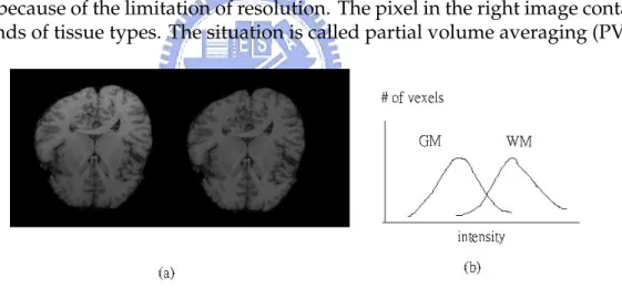
2. Partial volume averaging (PVA): : There is more than one tissue within one voxel. It is caused by the finite spatial resolution of the MR imaging system. Figure 1.4 illustrates how a voxel in the boundary contains more than one tissue type because for the finite resolution.

1.1 Background 5

Figure 1.2: A 3-D magnetic resonance image of human head. It is shown in coronal, sagittal and axial views.

the Radio-Frequency (RF) gain in the RF coil, so the intensities associated with these two tissues overlap. Figure 1.5 shows an example of MRI with inhomogeneities.

4. Convolution and variability of the brain: The nature of cortex is complicated and highly convoluted. The morphologic shape defers from subject to subject. Age,sex and even some disease influence the structure of cerebral cortex.

5.Topology preservation: The topology must be considered for some application such as brain functional mapping. The topology of the cortex is that of two crumpled sheets having no holes of self intersections.

Besides accuracy, a well cortex segmentation have to be robust. A cortex segmen-tation system are not just used for one subject. It have to deal with the images for subjects with different sex, age and even have some disease that effect the cortex structure. It also have to be robust to the noise produced by the MR imaging system such as random noise, intensity inhomogeneities. Efficiency is an important issue when techniques that let the segmentation robust are applied.

1.1.4

Applications of Cortex Segmentation

The cortex changes over time, as in aging, Alzheimer disease, or developmental disorders. Thus, many anatomy analyses focus on the cortex. Extracted cerebral cortex can be measured to get much useful information. This information helps the research in pathology prediction, determining morphological and structure changes or deformation. It also helps quantitative assessment of brain disease and treatment procedures.

Cortex segmentation also helps brain functional mapping. The location of functional activity obtained from positron emission tomography (PET), functional magnetic resonance imaging (fMRI), or magnetoencephalography (MEG) can be mapped to the extracted cortical surface, providing a better understanding of brain function and organization. For that purpose, we have to visualize the cortex and

1.1 Background 7

Figure 1.4: The four boundary pixels in the left image become one in the right image because of the limitation of resolution. The pixel in the right image contains two kinds of tissue types. The situation is called partial volume averaging (PVA).

Figure 1.5: (a) It shows the MRI with inhomogeneities (left) and normal MRI (right). Obviously,the intensities of the WM in the upper are brighter than those in the bottom. (b) The distributions of GM and WM overlap. For some voxels in GM, the intensities are brighter than some voxels in WM.

cortex segmentation is the first step. We can visualize the cortical surface in 3-D or create a flattened representation of the cortical surface.

1.2 Related Works 9

1.2

Related Works

A significant number of approaches have been proposed to deal with this prob-lem. There are several survey papers in the area of cortex segmentation [1] [2] [3]. These approaches can be roughly classified into three main categories:

1. Region-based approaches 2. Reformable model approaches 3. Hybrid approaches.

Some methods also take advantage of the cortical structure information as the constraint to improve the segmentation result.

1.2.1

Region-Based Approaches

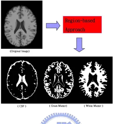
These kind of approaches segment image into different regions depending on the underlying consistency of any relevant feature in different regions. Figure 1.6 illustrates a example of results in region-based approaches.

The thresholding-based approach is the most intuitive approach [4]. The dif-ficulty is determining the value of the thresholds. A seed-growing approach is proposed by Cline [5]. Voxels around the seed are included in the region if they are sufficiently similar to the voxels already in the region. In the seed-growing approach, only well-defined regions can be robustly identified. Atlas-based ap-proaches use the brain atlas as a priori knowledge for segmentation.Images are registered to a brain atlas which had been segmented to get the probability map containing the probabilities for each voxel belongs to some tissue types. In multi-spectral segmentation that takes advantage the images acquired with multiple sequence, pattern recognition methods are often used. Supervised pattern recogni-tion methods assume that the number of classes and their intensity properties are known. This kind of approach is also called “tissue classification”. Those tissue classification approaches assume particular distribution of the features are called parametric including Expectation Maximization EM classification [6], Bayesian

Figure 1.6: The original image is segmented into different tissue classes in a region-based approach. The result of segmentation are images for CSF,WM and GM.

classification [7] ,Markov Random Field (MRF) classification [8]. Non-parametric approaches, such as k-nearest neighbors (KNN) [9],rely on the actual distribution of the training samples. The disadvantage of tissue classification approaches is that the number of classes mush be known in advance. Un-supervised pattern recognition methods are also called “cluster”. A paper on Adaptive Fuzzy C Mean (AFCM) was published by Pham [10]. In clustering approaches, a voxel could belong to one or more class by computing the fuzzy member function. Clustering approaches are time-consuming and depend on large number of user parameters. The advantage of region-based approaches is that they can take advantage of the priori knowledge to get better result. Because of partial volume averaging, region-base techniques suffer from misclassification of voxels and it is difficult to achieve crisp regions. The intensity inhomogeneity problem also has great influence on region-based approaches.

1.2 Related Works 11

Figure 1.7: In a deformable model, the output of segmentation are inner (GM/WM) and outer (CSF/GM) surfaces of the cortial cortex.The cortex can be reconstructed from these two surface.(The resulting surfaces are from [11] )

1.2.2

Deformable model approaches

These approaches estimate the inner and outer surface of the cerebral cortex depending on the gradient features of the image.An initial surface is given in deformable model approaches. The surface moves and stops in the boundary. Figure 1.7 illustrates a example of results in deformable model approaches. There are two kinds of deformable models:

1. Parametric deformable model approaches: Snake (active contour) is proposed by Kass, Witkin and Terzopulos [12]. Snake is an energy-minimizing spline that were pulled toward the image features such as lines and edges by the external and image force. Snake is also called parametric deformable model. There are much publications (ex. [13]) in the area of cortex segmentation with parametric deformable model. The speed term in this kinds of approaches was a very important issue. Snakes often suffer from the problem that the

stopping term was not robust and pulling force is not strong enough. Dealing with topology problems such as split and merge is also a great challenge for snakes.

2. Geometric deformable model approaches: It was in 1988 that Sethian’s PhD thesis [14] brought another revolution in image segmentation. Level set method is a numerical method. Sethian derived a level set function that changes over time. We will interchange the “level set function” with the “speed term” and find the “zero level set curve” as the propagating front. The detail of level set method will be discussed later. Casselles and Malladi [15] use geometric deformable model for segmentation. The advantage of level set method comparing to snakes is that it can handle topology problems such as split and merge.

Speed term is a very important issue for both snake approaches and level set approaches. A well defined speed term result in a surface stopping in the boundary. Speed terms that only use the gradient feature of the image are not enough. More information such as intensity distribution, cortex structure information are needed.

1.2.3

Hybrid approaches

The reason for this kind of approaches is to take advantage the local or global information for pulling or pushing snakes or level set method to capture the inner and outer surface. Incorporating such regional statistics, also called regularisers, makes the overall system more robust and accurate. Recently, more and more cortex segmentation researchers work on this kind of approaches [16] [17] [11] [18]. For this kind of approaches, efficient is an important issue. For example, clus-tering is time consuming, and we can use some techniques such as fast level set method to improve it.

1.2 Related Works 13

1.2.4

Approaches using cortical structure information

Recently, there have been some efforts to use constrains due to cortical structure information. Teo [19] used the fact that white matter is connected as constrain to grow surface from white matter. Davatzikos [20] used the homogeneity of intensity levels within the gray matter region to introduce a force that drive the deformable surface toward the center of gray matter layer. MacDonald [21] used an inter-surface proximity constraint in a two inter-surface model of the inner and outer cortex surface in order to guarantee that the surfaces do not intersect themselves.

Zeng [22] used the fact that the thickness of cortex is nearly constant. Zeng developed a coupled surface model that propagate two surface at the same time and designed a specific speed term that force the two surface remaining a certain distance. Following the coupled surface model suggest by Zeng [22], Goldenberg proposed a model using a variation geometric framework. It is based on advanced numerical schemes for surface evolution that yield a geometrically consistent and computationally efficient technique. The coupled surface model has showed their success in both accuracy and efficiency.

Chapter 2

Method

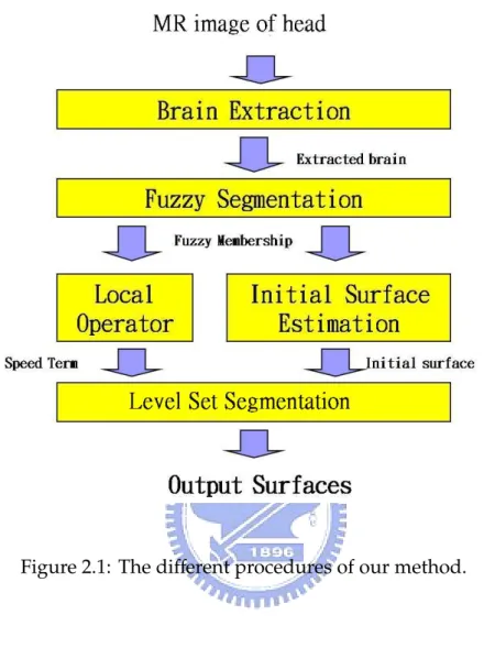
Figure 2.1: The different procedures of our method.

2.1

Overview

In our section,we introduce the overview of our method. A hybrid cortex segmentation method is used in our these. Figure 2.1 shows the procedures of our method. First, non-brain tissue types is removed from the original image. Fuzzy segmentation step provides the fuzzy membership from. The fuzzy membership was fed to local operator the get the speed term for segmentation step. Initial surface was estimated form WM fuzzy membership. Finally, level set method was used to propagate the initial surface to the boundary of inner (WM/GM) and outer (CSF/GM) surface.

2.2 Brain Extraction 17

Figure 2.2: A simple illustration of the merging process. A basin is merged into a deeper basin, if and only if its depth relative to the current voxel intensity is less than or equal to the preflooding height. (This figure is cited form [23])

2.2

Brain Extraction

Brain extraction, also called skull stripping, is an important and basic technique for the cortex segmentation and many analysis of neuron imaging data. The goal of the brain extraction step is to extract an initial brain volume, removing most of the non-brain tissue, such as scalp, skull, eyeball... In our thesis we adapt the watershed method proposed by Hahn and Peitgen [23].

The basic assumption of the watershed algorithm is the connectivity of the white matter. Because darker gray matter and even darker CSF surround the connected white matter, this region can be interpreted as the top of a hill in a three-dimensional virtual landscape. We consider the inverted gray level MR images that the WM hill become a valley. Two points are “connected” if there is a connectivity path that contain a lower intensity than the darker of the two points up to a maximum difference: the preflooding height, hp f . The watershed transform was applied to test the connectivity of whole volume image.

The first step of the watershed algorithm is the sorting of all voxels (of the gray level inverted image) according to their intensity. Then, we process each voxel in ascending order :

If the voxel does not have any already processed neighbors in its three-dimensional( 6-neighborhood), a new basin is formed. This voxel represents a local intensity minimum.

If the voxel has one or more processed neighbor, “Voxel-basin merging” is applied to the voxel : Merge the voxel with the basin with the darkest bottom voxel.

If two or more neighbors have already been processed belonging to different basins, these are tested for “basin-basin merging”: All the neighboring basins whose depth relative to the current voxel intensity is less than or equal to the preflooding height hpf will be merged with the same basin as the voxel itself, i.e., the deepest neighboring basin. Figure 2.2 illustrates the merging process of the watershed method.

After the watershed transform with an appropriate preflooding height hpf, one basin should exist that represents the whole brain. However, the result image is often inaccurate. The brain may be split in two or more basins. The brain radius was estimated before watershed transform. If the main basin is significantly small than estimated volume, we combine the basins to a reasonable size.

2.3

Fuzzy Segmentation

In the fuzzy classification,the voxels may be classified into multiple classes with a varying degree of membership. The fuzzy membership also gives an indication of where noise and partial averaging have occurred in the image. In stead of standard fuzzy c-mean.In our thesis, we adopt a slice-by-slice 3-D adaptive fuzzy C-means (AFCM) method. Based on fuzzy C-means (FCM) method, AFCM is robust to intensity inhomogeneities by calculating a smooth gain field.In our thesis, we extend 2-D AFCM to a slice-by-slice 3-D AFCM because of the efficiency issue.

2.3 Fuzzy Segmentation 19

2.3.1

Adaptive Fuzzy c-means Method

Here, we only introduce the algorithm for 2-D AFCM, the detail can be found in [10]. AFCM cluster the data by computing the fuzzy membership for each voxel in the image for a specified number of classes. The fuzzy membership, constrained be between zero an one, reflects the similarity between the data value at that location and the prototypical data value or centroid, of its class.

Suppose that Ω is the set of voxel locations in the image domain, ujk is the

membership value at voxel loaction j for class k (the total number of classes C is assumed to be known), yj is the observed image intensity at the location j, gjis the

gain field at location j, and vkis the centroid of class k. The algorithm of AFCM are

as below:

1. Provide initial value for the centroid, vk, for k=1...C, and set gj = 1 for all

j ∈Ω.

2. Compute the membership as follows: ujk=

k_yj−_gjvkk−2

PC

l kyj−gjvlk−2

for all j ∈Ω and k=1...C and k.k is the inner product operator. 3. Compute new centroids as follows:

vk = P j∈Ωujkgjyj P j∈Ωujkg2_j for k= 1...C

4. Compute the new gain field by solving the following space-varying difference equation for gi C X k=1 ujk < yj, vk >= gj C X k=1 ujk< vk, vk > +λ1(H1∗g)j+ λ2(H2∗g)j

This equation is soluved iteratively using the Jacobi or Gaussian-Seidel schemes, the details can be found in [10]. Standard finite difference were used comput-ing the convolution kernels H1 and H2. For 2-D images the resulting kernels

are: H1 =              0 −1 0 0 4 −1 0 −1 0              H2 =                          0 −1 0 0 2 0 2 −8 2 0 1 −8 20 −8 1 0 2 −8 2 0 0 0 1 0 0                         

5. If the algorithm has converged, the quit. Otherwise, go the Step 2.

A proper estimation of intimal values of the centroids will improve the accuracy and convergence of the algorithm. The parameterλ1and λ2are set to let the gain

field smooth. Ifλ1andλ2are set sufficiently large, the AFCM reduces to FCM.

2.3.2

Modified Adaptive Fuzzy c-means Method

In our method, we have to apply AFCM to 3-D volume brain image. However, 3-D Adaptive Fuzzy c-means Method was extremely time consuming because of the calculating of 3-D gain field. We propose a slice-by-slice AFCM in our method. Our assumption of modified AFCM is that the inhomogeneity artifact changes slowly in the spatial domain. The distributions of neighboring slices are very close. The first step of modified AFCM is to calculate the distribution of some slices in the middle of brain. Second, apply AFCM to the middle slices with the information derived from previous step. Finally, apply AFCM to every slice from middle slices with the information of neighbor slices.

2.4 Local Operator 21

Since the information of neighbor slices reduces the iteration number for the convergence of the gain field, modified AFCM is efficient. Processing the image slice-by-slice solve the inhomogeneity in z-axis.

2.4

Local Operator

The speed term is a very important part in deformable model segmentation. It determines where the moving surface stop. Unlike the active contour approaches, level set approaches do not need pulling force. The requirement of speed term is that the speed is high in the region of tissues and zero in the boundary.

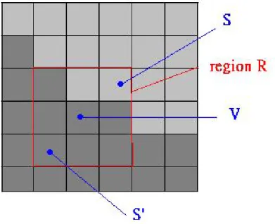
The fuzzy memberships are not directly in our method. If the speed term for a voxel only use the information itself, the boundary will be confused. Local operator is often applied to take advantage the information of nearby region. For example, Gaussian operator and Laplacian operator are also kinds of local operator. Consider a voxel v in the boundary of GM and WM. S is a voxel in the region R and s0

is at the opposite side to v (See Figure 2.3). The probability S ∈ WM and S0 _∈

GM are both high. Based on this idea, the probability for v belong to inner surface and outer surface are :

P(v ∈ innersur f ace)= P s∈R[P(S ∈ WM) ∗ P(S 0 _∈ GM)] P S∈R P(v ∈ outersur f ace)= P s∈R[P(S ∈ CSF) ∗ P(S 0 _∈ GM)] P S∈R

The probability that a voxel belonging to each tissue type is calculate by the fuzzy member function of fuzzy segmentation step. We separate the equation into two parts s = v and s , v. For example, consider a voxel v in the boundary of outer surface. In different direction of boundary, there are always some value of pairs of P(S ∈ CSF) ∗ P(S0 _∈

GM) are high. If v is exactly the boundary voxel, v contains both CSF and GM. Thus the value of P(v ∈ CSF) ∗ P(v0 _∈

GM) is also high. We invert the result of local operator and apply some transformation to let the result smooth and the value are between 0 to 1. Thus, the speed term is high in the tissue type and approaches zero at the boundary.

Figure 2.3: An example of local operator in our thesis.

2.5

Initial Surface

A proper initial surface is very important to segmentation with deformable model approaches for the efficiency and accuracy purpose. Initial surface close the boundary will reduce the numbers of iteration in level set segmentation. With Initial surface outside the cortical surface, the deformable model have difficulty progressing into the sulci. Initial surface inside the surface is better than in outside. With the fact that white matter is connected, we estimate the surface of WM as the initial outer surface and shrink it to get inner initial surface. We do so by smoothing the WM fuzzy membership and applying isosurface approach on it. Removing disconnected parts and filling operation are essential before applying isosurface approach.

2.6 Level Set Method 23

Figure 2.4: Level set formulation of equation of motion - (a) and (b) show the curve γ(t = 0) and the surface at Ψ(x, y) t=0, and (c) and (d) show the curve γ(t) and the surfaceΨ(x, y) at time t.(This figure is cited from [15])

2.6

Level Set Method

The level set method is a powerful numerical technique developed in the 1988 by the American mathematicians Stanley Osher and James Sethian [14].It has be-come popular in many disciplines, such as image processing, computer graphics, computational geometry, optimization, and computational fluid dynamics.The es-sential idea of the level set methods is to represent the propagating surface (in our case) of interest as a front and embed this front as the zero level set of a higher dimensional function defined by where is the signed distance from position to. An Eulerian formulation is produced for the motion of this surface, propagating along its normal direction with speed where can be a function of the surface characteristics (such as the curvature, normal direction, etc.) and the background characteristics (e.g., gray level and gradient in the images, etc.).

The motivation of level set method is to track the motion of an propagating interface. Consider a closed curve moving in the plain. Letγ(0) be a smooth,closed

Figure 2.5: An example of level set method (from http://en.wikipedia.org/wiki/).

initial curve in the Euclidean plain R2_{. This initial curve moves along its normal}

vector field with speed term K which describes the speed of each point on the curve. Letγ(t) be the one-parametric family of curves generated by moving γ(0) along its normal vector field.

The main idea of level set approaches is to embedded the propagating interface as the zero level set of a higher dimension function Ψ. Let Ψ(x, y, t = 0), where x ∈ Rn_{is defined by}

Ψ(x, y, t = 0) = d

where d is the distance from (x,y) toγ(t = 0), d is positive (negative) if x is outside (inside) the curve γ(t = 0). The closed curve can be represented as the level set Ψ = 0 of the function Ψ.Thus, we have the initial function Ψ(x, y, t = 0) with the property that

γ(t = 0) = {(x, y)|Ψ(x, y, t = 0) = 0}

As illustration,consider a expanding circle.Suppose the initial curve γ(t = 0) is a circle in the xy-plain(Figure 2.4(a)).We image the circle is the level setΨ = 0 of an initial surface z= Ψ(x, y, t = 0) in R3_{(Figure 2.4(b)).We can match moving curveγ(t)}

2.6 Level Set Method 25

Figure 2.6: An example of estimating the curve from the level set function.

yield the moving curve(Figure 2.4(c)and(d)).

With the speed function F(x, y, t),the evolution equation for the level set function Ψ can be represented by means of a so-called Hamilton-Jacobi equation :

Ψt+ F|OΨ| = 0

This is a partial differential equation, and can be solved numerically, for example by using finite differences on a Cartesian grid.

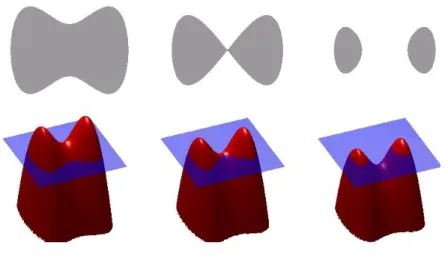
Figure 2.5 shows another example of level set method. In the upper-left,there is a closed curve moving toward inside the curve along its normal vector field. We can see that the curve changes topology by splitting in two. It would be quite hard to describe this transformation numerically by parameterizing the curve and following its evolution. In the below, the red surface is the graph of a level set function for the curve, and the flat blue region represents the x-y plane. We can see that it is much easier to track the curve through the evolving level set function.

2.6.1

Approximation for Level Set Method

One of the advantages of the Hamilton-Jacobi equation is that the evolving functionΨ(x, y, t) remains a function as long as F is smooth. Thus,we could use a discrete grid in the domain R2_{and substitute finite difference approximation for the}

spatial and temporal derivatives. For example, using a uniform mesh or spacing h, with grid node ij, and employing the standard notation thatΨn

i jis approximation

to the solutionΨ(ih, jh, n M t),where M t is the time step, we may write : Ψn+1

i j −Ψni j

M t + (F)(Oi jΨ

n i j)= 0

Here we have used forward differences in time,and let Oi jΨn_{i j}be some appropriate

finite difference operator for the spatial derivative. With a given initial curve, the initial value Ψ0

i j for each grid can be computed

by calculating the distance from each grid to the initial curve. Thus,the value of can be computed iteratively through the following equation:

Ψn+1 i j = Ψ n i j+ M t((F)(Oi jΨ n i j))

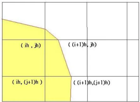
The moving curve at time n M t can be estimated from Ψn

i jof all grids.We may

deter-mine if the curve pass through a grid by checking the sigh ofΨn_{near the grid, and}

computing where the curve passes through by interpolation. Figure 2.6 shows that the curve pass through the grid (ih,jh) whereΨn

i j< 0,PΨi(j+1) < 0,Ψ(i+1)j > 0,Ψi(j+1) > 0.

2.6.2

Speed Term

The speed term F in the level set approaches is usually a function of curvature and has the form:

F(K)= F0+ F1(K)

The term F1(K) is dependent on the geometry of the moving curve,such as its

local curvature.This term smoothes out the high curvature region of the moving curve. The curvature is easily obtained from the divergence of the gradient of the

2.6 Level Set Method 27

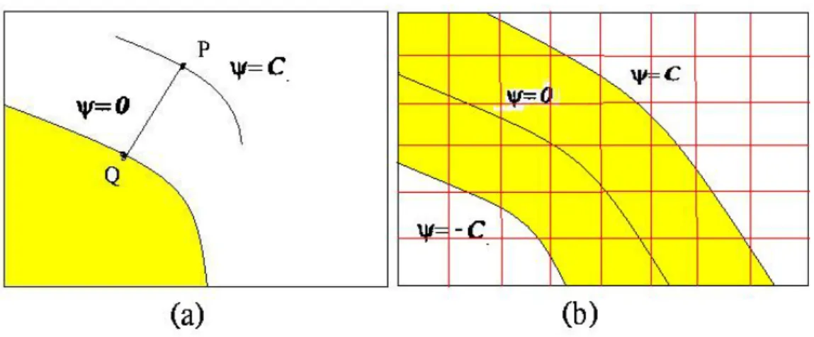
Figure 2.7: (a) It shows that the speed at Q is extended to Q. (b) It shows the grid points in the yellow area are added to narrow band set.

unit local vector,that is, K= ∇_|∇∇Ψ Ψ = − ΨxxΨ2y− 2ΨxΨyΨxy+ ΨyyΨ2x (Ψ2 x+ Ψ2y) 2 3

The advection component F0is independent to the moving curve’s geometry.In

image segmentation, the speed term F0 is a image-based speed function and

de-signed to force the curve stop in the boundary of the shape. We have to extend the speed function on the zero level set to other level sets to prevent collide. Imagine that the point P withΨn

p = C in the figure 2.7(a) remains unchanged and the curve

propagate. Then Ψ = 0 and Ψ = C collide. We construct the extension of speed function by letting the speed at the point P be the speed at a point Q,such that Q is closest to P and lies on the level setΨ = 0.

Computation of the extension of image-based speed term is the most expensive step in these approaches. The closest point lying onΨ = 0 for each grid point needs to be computed in every iteration.

2.6.3

Narrow Band

Updating the level set function of all grid points is very time consuming and not necessary. Since we only focus on the zero level set , the grids too far away

Figure 2.8: The flowchart for the 3-D segmentation using level set method.

from the zero level set have no need to be updated. A grid set called “narrow band” was constructed.With a given constant C, he grids with |Ψ| < C were add to narrow band set.In figure 2.7(b), the gird points in the yellow region are added to the narrow band set.

Only grids in the narrow band set are updated in each iteration. The computa-tion of extension of speed funccomputa-tion reduces largely. If the zero level set is too close to the boundary of the narrow band, the narrow band have to be reconstruct and the grids in the narrow band have to be reinitialized according to the current zero level set.

2.6 Level Set Method 29

2.6.4

Segmentation with level set method

In our thesis, we consider the level set method in 3-D. Figure 2.8 shows the flowchart of the segmentation with level set method. The details of each steps are as following :

Initialization With a initial surface,the initial level set functionΨ is computed as the signed distance from grid to the initial surface. The initial surface is the current zero level set surface. For each grid point, the closest point that lies on the initial surface has to be computed.

Construct Narrow Band Construct a narrow band set and add the grid points with |Ψ| < C to the set. The parameter C is given according to the parameter M t to prevent the zero level set surface and narrow band boundary collide. If the set is reconstructed, theΨ function need to be reinitialized according to the current surfaceΨ = 0.

UpdateΨ function Update the grid points in the narrow band set with the

updat-ing equation: Ψn+1 i jk = Ψ n i jk+ M t((Fi+ Fc(K))(Oi jkΨ n i jk))

The extension image-based speed term Fiis well designed to stop the surface

in the boundary of shape. The curvature term Fc is also considered to let

the surface smooth. A proper value of M t is very important.This parameter control the propagating speed of the surface. The value of M t is a trade-off between efficiency and accuracy.

Find zero level set Apply isosurface approach to the currentΦ function,the result-ing surface is the current zero level set surface. This step also compute the closest points for the extension speed term.

Convergence Test if max(|Ψn+1_{i jk} −Ψn+1

i jk |)< ε with a given constant ε, the

segmenta-tion stop and output the current zero level surface. Otherwise, go the “Find zero level set” step.

Chapter 3

Results

Table 3.1: Basic data for MRI subjects. Step Sex Age Subject A Male 24 Subject B Male 43 Subject C Male 33 Subject D Female 30 Subject E Female 50

3.1

Materials

In our work,Magnetic resonance images of all normal subjects were acquired from the same 1.5T Siemens scanner at the Taipei Veterans General Hospital, which used a T1-weighted 3-D IR sequence with TR= 9.72ms, TE= 4ms, FA = 12, matrix size= 256x256, slices = 128, voxel size = 0.9x0.9x1.5mm3_{. Figure 3.1 shows 12 slices}

of MR images of subject A.

In our thesis, MR images of five subjects are used. They are marked as A,B,C,D,and E. The basic data of subjects are show in Table 3.1. We take sub-ject A for example in the next section.

3.2 Results of Each Steps 33

3.2

Results of Each Steps

In this section, we show the results of each step in our method, including brain extraction, fuzzy memberships, initial surfaces, and the result of cortical surfaces. We take the MR images of subject A for example in this section.

The first step of cortex segmentation is brain extraction. Non-brain tissue types are removed in this step. In our method, the original MR brain images are applied watershed method with a given paremeter Hp f . Figure 3.2 shows the images of extracted brain. The reulst of brain extraction step depend on the value of preflooding height Hp f . This value can be roughly estimated automatically from the intensity distribution (about 35 in our examples). If the value of Hp f is too high, mis-segmentation occurs. Otherwise, over-segmentation occurs. A little bit of over-segmentaton would not effect the results in our method. Thus, we use the value of Hp f that is higher (about 40) than estimated value to prevent missing brain tissues. We can see that some non-brain tissue types are left in Figure 3.2. We also applly the skull stripping function (brain extraction) in MRIcro to the MR images. Figure 3.3 show the extracted brain of MRIcro. Some brain tissues are missing after brain extraction.

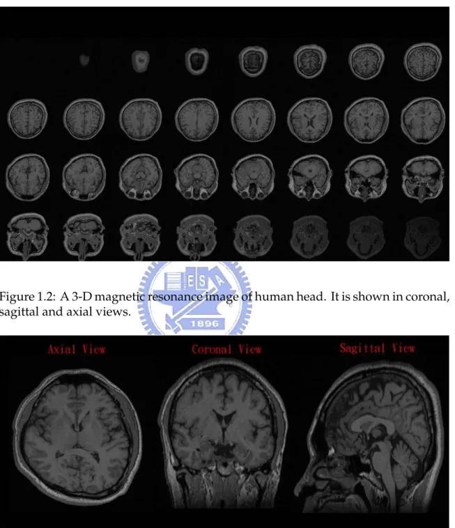
The proposed slice-by-slice AFCM are applied to the extracted brain images to estimate fuzzy memberships. We assume there are three classes (CSF,GM, and WM) in the images. The voxels in the background are not counted in our method. The fuzzy meberships for CSF,GM and WM are shown in Figure 3.4, Figure 3.5, and Figure 3.6 separately (fuzzy memberships are scaled to the range between 0 to 255). The fuzzy memebership of a voxel indicates the degree it belong to a tissue type (ex. GM). We can see that the voxels in the boundary sometime have equal fuzzy membership of two tissue types. Random noise also cause the errors in fuzzy memberships. Thus, we can not use the fuzzy memberships directly.

The proposed local operator are applied to take advantage of the information of neighboring voxels. This local operator indicates the boundary of the cortex against noise. A local operator with kernel size 3x3x3 are applied to fuzzy memberships to estimate speed terms for inner surface (Fig. 3.7) and outer surface (Fig. 3.8). The

Figure 3.1: 12 slices of a brain MR image.

3.2 Results of Each Steps 35

Figure 3.3: This figure shows the extracted brain from MRIcro. The red circles indicate some brain tissues are missing after brain extraction.

intensity value for a voxel means the degree it belongs to the boundary. In level set segmentation, the surface will stop in the voxels with high intensity in Fig. 3.7 and Fig. 3.8. We can see that the boundary is clear after applying local operator and the noise is also removed(see Figure 3.9).

Figure 3.11 shows the estimated initial outer surface. This initial surface are estimated from WM fuzzy membership. The inner initial surface (See fig. 3.10) is estimated by shrinking the outer initial surface. The distance between two initial surface is about 3mm..

According the speed term and initial surfaces, the level set method estimate inner and outer surface of the cortex. Figure 3.12 and figure 3.13 the results of inner and outer cortical surface by using the proposed level set segmentation. In level set segmentation, the parameter time step M t influence the accuracy of results and numbers of iterations for convergence. We use M t = 0.2 in this example, and this means the surface moves at most 0.2mm in a iteration. We measure the maximum change ofΦ function in each iteration. If the maximum change is smaller than a

Figure 3.4: Fuzzy memebership for cerebral spinal fluid of subject A.

threshold, the level set segmentation stop. The current zero level set surface is the result. We estimate inner and outer surface in different deformable models. It takes about 50-60 iterations to convergence in our examples. We use a full resolution level set method in our method.

3.2 Results of Each Steps 37

Figure 3.5: Fuzzy memebership for gray matter of subject A.

Figure 3.7: This figure shows the speed term used for estimating inner surface.

3.2 Results of Each Steps 39

Figure 3.9: The boundary is clear after applying local operator. The noise is removed in speed term.

Figure 3.10: Estimated initial inner surface of subject A in different views.

3.2 Results of Each Steps 41

3.3 2-D Overlay of Reconstructed Cortical Surface on T1 images 43

3.3

2-D Overlay of Reconstructed Cortical Surface on

T1 images

In this section, we overlay the reconstructed cortex surface on the extracted brain images. In level set segmentation, the surface is determined by applying isosurface with isovalue= 0 to the value of level set function. The voxel inside the surface has a negative value of level set function. Thus, we can determine the region inside the surface by checking the voxels with negative value of level set function. In figure 3.15, we overlay the region inside the outer surface to the extracted brain images. In figure 3.14, we overlay the region inside the inner surface to the brain images. The constructed cortex lies inside the outer surface and outside the inner surface . Figure 3.17 shows the reconstructed cortex overlaid to the extracted brain images. With this step, we can verify the results of the proposed cortex segmentation. The result of outer surface is better than the result of inner surface. The inner surface is hard to reach the tiny region of WM. The non-brain tissues which are not removed in brain extraction step are not in the reconstructed cortex.

Figure 3.18, 3.20, 3.22, and 3.24 shows the extracted brain images for subject B,C,D, and E respectively. Figure 3.19, 3.21, 3.23, and 3.25 shows the reconstructed cortex regions overlaid to extracted brain images of subject B,C,D, and E.

Figure 3.14: In this picture,we overlay the region inside the inner surface to the extracted brain of subject A.

Figure 3.15: In this picture,we overlay the region inside the outer surface to the extracted brain of subject A.

3.3 2-D Overlay of Reconstructed Cortical Surface on T1 images 45

Figure 3.17: In this picture,we overlay the reconstructed cortex region of subject A to the extracted brain of subject A.

3.3 2-D Overlay of Reconstructed Cortical Surface on T1 images 47

Figure 3.18: Extracted brain image of subject B.

Figure 3.19: Reconstructed cortex region overlaid to the extracted brain of subject B.

Figure 3.20: Extracted brain image of subject C.

Figure 3.21: Reconstructed cortex region overlaid to the extracted brain of subject C.

3.3 2-D Overlay of Reconstructed Cortical Surface on T1 images 49

Figure 3.22: Extracted brain image of subject D.

Figure 3.23: Reconstructed cortex region overlayed to the extracted brain of subject D.

Figure 3.24: Extracted brain image of subject E.

Figure 3.25: Reconstructed cortex region overlaid to the extracted brain of subject E.

3.4 Result on Simulated MR Data with Ground Truth 51

3.4

Result on Simulated MR Data with Ground Truth

In this section, we apply our method to simulated MR images. These simulated MR images are downloaded from Brain Web (http://www.bic.mni.mcgill.ca/brainweb/). These data contains simulated brain MRI data based on two anatomical models: normal and multiple sclerosis (MS). For both of these, full 3-dimensional data vol-umes have been simulated using three sequences (T1-, T2-, and proton-density-(PD-) weighted) and a variety of slice thicknesses, noise levels, and levels of in-tensity non-uniformity (inhomogeneity). In our these we use the T1-weighted simulated images for normal model with matrix size= 217x181, slices = 181, and voxel size= 1mm3_.

We apply our method to five simulated MR data with different noise levels and levels of intensity non-uniformity. We compare the reconstructed cortex with the ground truth. We evaluate as follow. We define number of voxel in ground truth as Ng and number of voxels in reconstructed cortex as Nr. Nrg is the number of

voxels in both ground truth and reconstructed cortex. Nrg0 is the number of voxels

in reconstructed cortex but not in ground truth. A true positive (TP) rate is defined as Nrg/Ngwhile the false positive (FP) rate is defined as Nrg0/N

r

Table 3.2 shows the value of TF rate and FP rate for cortex segmentation in simulated MR images with different level of noise and non-uniform. The FP rate is relative high with higher noise level. Inner surface can not move into thin area of WM with high noise level. Intensity non-uniform result in weak speed term. The surface may stop in the wrong boundary.

3.5

Discussion on Reconstructed Cortex

In this section, we discuss about the results of our method. There are no standard method for us to measure the performance of cortex segmentation. The segmentation works well on most regions, but some bad segmentation exist. We point out the bad segmentation visually and discuss why it happens. These bad segmentation are classified into three classes:

Table 3.2: It show the value of TP rate and FP rate for images with different level of noise and non-uniform.

Level of noise and non-uniform TPrate FPrate 3œNoise and 0œNon-Uniform 98.9 1.6 7œNoise and 0œNon-Uniform 96.7 5.5 0œNoise and 20œNon-Uniform 97.5 2.1 0œNoise and 40œNon-Uniform 93.5 4.9 3œNoise and 20œNon-Uniform 96.1 3.7

Problems in Speed Term The speed term does not indicated the correct bound-ary in some region. This often occurs in the region with thin white matter. For example, the red circles in bottom-left of Figure 3.26 indicate the incor-rect speed term. The incorincor-rect speed term results in incorincor-rect segmentation (bottom-right of Figure 3.26). Local operator does not work well in a tiny region with voxels with ambiguous fuzzy memberships(see top of Figure 3.26).

Problems in Level Set Segmentation Sometimes, the speed term is correct but the result of level set segmentation is incorrect. This often occurs when propagating the inner surface to thin WM between GM. In figure 3.27, the red circles show this incorrect segmentation. The reason of this problem may be the incorrect extension of speed term. Another reason is the resolution of level set method. Computation error of estimating in level set method is also possible reason.

Problems in Topology The surfaces in level set methods are merged if these two surface are very close. It is not the problem of speed term. It is because of the nature of level set segmentation. The topology of surfaces have to be preserved if the result surface are used for visualization and mapping the functional information. Figure 3.28 shows this situation.

3.6 Computation Time 53

Figure 3.26: An example for incorrect speed term.

3.6

Computation Time

The proposed method was tested on a PC equipped with Windows XP with processor 3.2GHz and 2GB RAM. The size of MRI volume data is 256X256X128. We run the level set method with full resolution. Note that time step is an important parameter in level set segmentation. With small time step, the result is more accurate but requires more iterations. With large time step, it takes less iterations but the result is coarse. We use an adaptive time step in our method. Time step is initialized as a large value (0.2). When the moving surface is close to the boundary (measured by the changes of level set function), time step is set to a smaller value (0.1). Adaptive time step is more efficient without losing accuracy.

Figure 3.27: An example for incorrect level set segmentation. The computation time for each step are shown in Table 3.3.

3.6 Computation Time 55

Figure 3.28: An example for incorrect topology.

Table 3.3: Computation time for each step of proposed method. step Computation Time (min) Brain Extraction 1

Fuzzy Segmentation 5-10 Local Operator 1

Initial Surface 1-2 Level Set Segmentation 50-60

Chapter 4

Conclusions

We have developed in this thesis a level set method for robust cortex segmen-tation in MR images. The cortex segmensegmen-tation method include brain extraction, fuzzy membership estimation, initial surface estimation, local operator for speed term and segmentation with level set method. Level set method is a numerical technique that can track the moving surface. We provided an initial surface and well-designed speed term to level set method, and obtain the cortical surface after iterations.

The major advantage of our method is its robustness. Estimating fuzzy mem-berships deals with the problem of partial volume averaging. Adaptive fuzzy C-means method are robust against intensity inhomogeneity estimating fuzzy mem-berships. Initial surface estimated from WM fuzzy membership are always close to the boundary in MR images of subjects with different brain morphology. Local operator which estimates the speed term with region information are robust to ran-dom noise and inhomogeneities. Another advantage of our method is its efficiency. The most time-consuming parts of our method are estimating fuzzy memberships and level set segmentation. Because original 3-D AFCM is very time-consuming, we used slice-by-slice AFCM to estimate fuzzy memberships against intensity in-homogeneities in 3-D. Information of neighboring slices provides good initial value used for AFMC of each slice. This accelerate the AFCM processes. The initial sur-face close to the boundary reduce the iteration of level set segmentation. We use narrow band to reduce the computation on updating the level set value of grid points.

We have applied our method to 5 brain MR images acquired from the same machine. The proposed cortex segmentation method works well without adjusting the parameters. The subjects of MR images are different and the noise distribution are also different. However, there is still a problem about accuracy in our method. The resulting surface is hard to reach the thin region. Better local operator or other constraint may be applied to improve the accuracy.

Bibliography

[1] L.P.Clarke. MRI segmentation:method and applications. Mag. Res. Img., 13(3):343–368, 1995.

[2] J.S. Suri. Computer vision and pattern recognition techniques for 2-d and 3-d MR cerebral cortical segmentation (part i): A state-of-the-art review. Pattern Analysis and Applications, 5:46–76, 2002.

[3] J.S. Suri. Computer vision and pattern recognition techniques for 2-d and 3-d mr cerebral cortical segmentation (part i): A state-of-the-art review. Pattern Analysis and Applications, 6:8–28, 2002.

[4] K.O.Lim and A. Pfefferbaum. Segmentation of mr brain images into cere-brospinal fluid spaces, white and gray matters. J Comput Assist Tomogr., 13(4):588–593, 1990.

[5] H.E Cline, W.E. Lorensen., and R. Kikims. Thre-dimensional segmentation of mr images of the head using probability and connectiveity. J Comput Assist Tomogr., 14:1037–1245, 1990.

[6] WWells III, WEL. Grimson, R. Kikinis, and FA. Jolesz. Adaptive segmentation of MRI data. IEEE Trans on Medical Imaging, 15(4):429–442, 1992.

[7] M. Joshi, J. Cui, K. Doolittle, S. Joshi, D. Van Essen, L. Wang, and MI. Miller. Brain segmentation and the generation of cortical surfaces. Neuroimage, 9(5):461–476, 1995.

[8] k. Held, E. Rota Kopps, B. Krause B, W. Wells, R. Kikinis, and H. Muller-Gartner. Markov random field segmentation of brain MR images. Neuroimage, 16(6):878–887, 1998.

[9] Alan C. Evans. A fully automatic and robust brain MRI tissue classification method. Med Img. Aanlysis., 7:513–527, 2003.

[10] C. Xu, D.L. Pham, M.E. Rettmann, D.N., and J.L. Prince. Reconstruction of the human cerebral cortex from magnetic resonance images. Medical Imaging, IEEE Transactions on, 18(6):467–480, 1999.

[11] C. Baillard, P. Hellier, and C. Barillot. Segmentation of 3-d brain structures using level sets. Research Report 1291 IRISA, Rennes Cedex, France, 2000.

[12] M. Kass, A. Witkin, and D. Terzopolous. Snakes: active contour models. International Conference on Computer Vision, pages 259–268, 1987.

[13] B. Fischl, MI Sereno, and AM Dale. Cortical surface-based analysis. i. segmen-tation and surface reconstruction. NeuroImage, 9(2):179–194, 1999.

[14] JA. Sethian. An analysis of flame propagation. PhD Thesis, Department of Mathematics, University of California, Berkeley,CA,, 1982.

[15] R. Malladi, JA. Sethian, and BC. Vemuri. Shape modeling with front prop-agation. IEEE Trans Pattern Analysis and Machine Intelligence, 17(2):158–175, 1995.

[16] C. Xu, D.L. Pham, M.E. Rettmann, D.N. Yu, and J.L. Prince. Reconstruction of the human cerebral cortex from magnetic resonance images. IEEE Transactions on Medical Imaging, 18(6):467–480, 1999.

[17] JS.Suri. White matter/gray matter boundary segmentation using geometric snakes: a fuzzy deformable model. International Conference in Application in Pattern Recognitiong, pages 11–14, 2001.

BIBLIOGRAPHY 61

[18] N. Paragios and R. Deriche. Coupled geodesic active regions for image seg-mentation. Eur. Conf. Computer Vision, 2000.

[19] P. C. Teo, G. Sapiro, and B. Wandell. Creating connected representations of cortical gray matter for functional MRI visualization. IEEE Transactions on Medical Imaging, 16:852–863, 1997.

[20] C. A. Davatzikos and R. N. Bryan. Using a deformable surface model to obtain a shape representation of the cortex. IEEE Transactions on Medical Imaging, 15:785–795, 1996.

[21] D. MacDonald, D. Avis, , and A. C. Evans. Multiple surface identification and matching in magnetic resonance images. Proc. SPIE, 2359:160–169, 1994. [22] X. Zeng, L. H. Staib, R. T. Schultz, and J. S. Duncan. Segmentation and

measure-ment of the cortex from 3-d MR images using coupled surface propagation. IEEE Transactions on Medical Imaging, 18:927–937, 1999.

[23] F. Segonne, A.M. Dale, E. Busa, M. Glessner, D. Salat., H.K. Hahn, and B. Fischl. A hybrid approach to the skull stripping problem in MRI. IEEE Transactions on Medical Imaging, 16(1):927–937, 1997.