國
立
交
通
大
學
資訊科學與工程研究所
碩
士
論
文
利用足跡分析來加速基於消失點射線取樣
之人群定位演算法
Acceleration of Vanishing Point-Based Line Sampling Scheme
for People Localization via Footstep Analysis
研 究 生:王之容
指導教授:莊仁輝 教授
利用足跡分析來加速基於消失點射線取樣之人群定位演算法
Acceleration of Vanishing Point-Based Line Sampling Scheme
for People Localization via Footstep Analysis
研 究 生:王之容 Student:Chih-Jung Wang
指導教授:莊仁輝 Advisor:Jen-Hui Chuang
國 立 交 通 大 學
資 訊 科 學 與 工 程 研 究 所
碩 士 論 文
A ThesisSubmitted to Institute of Computer Science and Engineering
College of Computer Science
National Chiao Tung University
in partial Fulfillment of the Requirements
for the Degree of
Master
in
Computer Science
July 2012
Hsinchu, Taiwan, Republic of China
i
利用足跡分析來加速基於消失點射線取樣之人群定位演算法
研究生:王之容
指導教授: 莊仁輝
國立交通大學資訊科學與工程研究所
摘要
近年來,以視覺為基礎的人群定位與追蹤越來越受到重視,也不斷發展出新的技術 與應用。然而,大部分的方法都需仰賴大量的計算方能處理嚴重遮蔽的問題,且往往需 倚賴特殊硬體才能達成即時的定位與追蹤。不同於這些研究,本論文提出一快速且準確 的多攝影機人群定位演算法,對前景區域建立以消失點為基礎的二維樣本線段,並將之 投影於地平面,利用足跡分析找出線段相交密集處,有效限縮人物立足點在地平面的可 能範圍。再透過二維前景影像,對人物立足點可能區域做進一步的篩選與驗證,有效率 地估計出人物的位置與高度。本篇論文不需大量分析人物特徵點,有效率地降低系統的 計算成本以符合即時運算的需求。經實驗證明,本篇論文演算法相較於先前研究[9]的人 物三維重建方法,在多人且嚴重遮蔽的環境中可提升至十倍計算速率,且依然不失偵測 正確度與定位精準度,進而達成即時的三維人群定位。ii
Acceleration of Vanishing Point-Based Line Sampling Scheme
for People Localization via Footstep Analysis
Student: Chih-Jung Wang
Advisor: Jen-Hui Chung
Institute of Computer Science and Engineering
National Chiao Tung University
ABSTRACT
With the popularity of vision-based camera surveillance, the research on people
localization appeals to much attention. In this study, we propose an efficient and effective
system capable of locating a crowd of dense people in real time, using multiple cameras. For
each camera view, line samples, originated from a vanishing point, of foreground objects are
projected on the ground plane. Ground regions containing a high density of projected lines are
then used to find people locations. Enhanced from previous works, the people localization
approach proposed in this study needs not project all foreground pixels of all views to
multiple reference planes or compute pairwise intersections of projected sample lines at
different heights, resulting in significant improvement in computational efficiency.
Furthermore, the people heights can also be estimated. Experimental results on real
surveillance scenes show that comparable accuracy in people localization can be achieved
iii
ACKNOWLEDGMENTS
I am heartily thankful to my advisor, Dr. Jen-Hui Chung, whose encouragement, guidance
and support from the initial to the final level enabled me to develop an understanding of the
subject.
I also want to extend my special thanks to the members of my dissertation committee, Dr.
Yen, Dr. Tsai, and Dr. Lai, for their thoughtful insights and comments to help develop this
research.
Special gratitude is also extended to the colleagues of the Intelligent System Laboratory at
National Chiao Tung University for their suggestions and help during my thesis study. I offer
my regards and blessings to all of those who supported me in any respect during the
completion of this research.
Lastly, I wish to express my heartfelt gratitude especially to my dear family and boyfriend
iv
CONTENTS
ABSTRACT (in Chinese) ... i
ABSTRACT (in English) ... ii
ACKNOWLEDGMENTS ... iii
CONTENTS ... iv
LIST OF FIGURES ... v
LIST OF TABLES ... viii
Chapter 1. Introduction ... 1
1.1 Motivation ... 1
1.2 Review of Related Works ... 3
1.3 Overview of Proposed Methods ... 5
1.4 Contributions of This Thesis ... 7
1.5 Thesis Organization ... 7
Chapter 2. Vanishing Point-Based Line Sampling and Projection ... 8
2.1 2D Line-Based Sampling from Vanishing Points ... 8
2.2 Line Projection via Ground Plane Homography ... 11
Chapter 3. Grid-Based Estimation of Candidate People Locations via Footstep Analysis ... 15
3.1 Grid-Based Discretization on Ground Plane ... 16
3.2 Candidate People Locations Estimation ... 19
Chapter 4. People Localization and Height Estimation ... 23
4.1 Refinement of 3D Line Samples ... 23
4.2 Generation of Major Axes of People ... 27
Chapter 5. Experimental Results ... 30
Chapter 6. Conclusions and Future Works ... 39
6.1 Conclusions ... 39
6.2 Future Works ... 39
v
LIST OF FIGURES
Figure 1.1 An example of isolated people in frame 185. (a) The frame before occlusion occurs. (b) The binary foreground image of (a). ... 1 Figure 1.2 An example of serious occlusion in frame 215. (a) The frame shows the person dressed in red jacket is occluded. (b) The binary foreground image of (a). ... 2 Figure 1.3 Multi-camera approach provides sufficient information for people localization. (a) The binary foreground images from four views of the same scene. (b) The localization result obtained from (a) by using our method. ... 2 Figure 1.4 Schematic diagram of the proposed people localization framework ... 6 Figure 2.1 Overview of the vanishing point-based line sampling and projection ... 8 Figure 2.2 Vertical poles on the ground plane intersect in the image at the vanishing point. .... 9 Figure 2.3 The 2D line-based sampling from vanishing point. (a) The original image of one view. (b) Foreground image of (a). (c) Vanishing point-originated line samples for (b). ... 10 Figure 2.4 Geometrical relationship between lines on image and on ground. ... 11 Figure 2.5 The 2D foreground line samples on image projected on ground. (a) Vanishing point-originated line samples in an image. (b) The projected 2D foreground line samples on the ground plane (top view). ... 12 Figure 2.6 An example of projecting 2D line samples from different views onto the ground plane. (a) Original images of multiple views. (b) Vanishing point-originated 2D foreground line samples for (a). (c) The projected 2D foreground line samples on ground plane for each view (top view). (d) The 2D foreground line samples from all camera views (the union of (c)). The actual people locations are shown as red points. ... 14 Figure 3.1 Overview of the grid-based estimation of candidate people locations. ... 15 Figure 3.2 The quantity of crossing line samples for each block is counted. ... 16 Figure 3.3 Result of the line counting for the first grid (layer 1) on the ground plane for the example shown in Figure 2.6. The numbers in each block represents the quantity of line samples crossing though it. ... 17 Figure 3.4 Result of the line counting for the second grid (layer 2) on the ground plane for the example shown in Figure 2.6. ... 17 Figure 3.5 Two grids with an offset of 25cm in both vertical and horizontal directions. ... 18 Figure 3.6 Close-up views of portions of Figure 3.3 and Figure 3.4 showing some line counts are dispersed among neighboring blocks. (a) The line count in the blue circled region is distributed in layer 1 (on the left), but is more concentrated in layer 2 (on the right). (b) The line count in the red circled region is more concentrated in layer 1, but is
vi
distributed in layer 2. ... 18
Figure 3.7 The two-layer grid occupancy map obtained by combining two grids (shown in Figure 3.3 and Figure 3.4). ... 19
Figure 3.8 The two-layered grids are merged into a quarter size grid by retaining the one with higher count. ... 19
Figure 3.9 The candidate people blocks (CPBs) for the example shown in Figure 3.7. ... 20
Figure 3.10 The illustration of generating four sample points in each CPB. ... 21
Figure 3.11 Sample points for the CPBs shown in Figure 3.9. ... 21
Figure 3.12 Projecting point at leg level hl to image view i. ... 22
Figure 3.13 The obtained CPLs for the example in Figure 3.11. ... 22
Figure 4.1 Overview of 3D people localization and height estimation ... 23
Figure 4.2 Generating and refining a 3D line sample... 24
Figure 4.3 An example of 2D refinement in each camera view i with one observed person. (a) The initial 3D line samples (red) and the refined ones (blue) in the binary foreground images of all views. (b) The initial 3D line samples (red) and the refined ones (blue) in the original images of all views. ... 25
Figure 4.4 The cross ratios CR(A, B, C, D) and CR’(A’, B’, C’, D’) are equal, since points A, B, C, D and A', B', C', D' are related by a projective transformation. ... 26
Figure 4.5 The relationship of the collinear points on 2D view i. (Please refer to Figure 4.2 for detailed relation between the 3D line sample and the projected one on image view i.) ... 26
Figure 4.6 Clustering and localization results after refinement and verification procedures for the example in Figure 3.13. (a) Input frame (9 persons). (b) Verified 3D line samples. (c) Top view of the clustering sets with red points representing the ground truth, and blue points representing the estimations, of people locations in this scene, respectively. (d) The 3D major axes (MAs). ... 29
Figure 5.1 An instance of sequence S1, frame 1 (9 persons, eight circling the center one). (a) Input frame from four different viewing directions. (b) Verified 3D line samples of different clusters in the scene. (c) 3D major axes (MAs) to represent different persons in the scene. (d) Localization results illustrated with bounding boxes. ... 31
Figure 5.2 An instance of sequence S2, frame 1 (9 persons, walking randomly). ... 32
Figure 5.3 An instance of sequence S3, frame 1 (12 persons, walking randomly). ... 33
Figure 5.4 An example of miss detection in sequence S2. (a) Segmented foreground regions and 2D line samples. (b) The localization results wherein the person with blue shirt cannot be detected because of the broken foreground region at his leg level. ... 35 Figure 5.5 An example of false alarms in sequence S2. (a) Segmented foreground regions and 2D line samples in all views. (b) The localization results illustrated with bounding boxes in all views. (c) The 3D MAs to represent different persons in the scene. The
vii
3D MA in red represents a false alarm. ... 35 Figure 5.6 An example of miss detections and false alarms in sequence S2. (a) The localization results illustrated with bounding boxes. (b) Clusters of verified 3D line samples in the scene with the circled region indicating the merge of two clusters. ... 36 Figure 5.7 Results of person height estimation for S1. ... 37 Figure 5.8 Results of person height estimation for S2. ... 37 Figure 5.9 Results of person height estimation for S3. ... 37
viii
LIST OF TABLES
Table 5.1 The information of three video sequences... 30
Table 5.2 Performance of the proposed approach ... 33
Table 5.3 Performance of people localization of [9] ... 36
Table 5.4 Results of person height estimation for S1. ... 38
Table 5.5 Results of person height estimation for S2. ... 38
1
Chapter 1. Introduction
1.1 Motivation
Recently, the proliferation of security surveillance cameras necessitates the development
of automatic/semi-automatic surveillance system with the assistance of computer technology.
Therefore, the research on vision-based people localization has been gaining popularity. In
more recent years, there has been a tremendous wave of interest in people localization for
crowded scenes. Serious occlusions may occur frequently within a group of people in a
real-world environment. Based on current research, there is still scope for accuracy and
efficiency improvements in solving occlusion problems.
Conventional people localization approaches are based on single-camera monitoring. A
target object can be successfully detected with a single static or moving camera if it is neither
occluded by nor occluding others in the scene. However, this kind of monocular approach
may not achieve high accuracy under serious occlusion. An example is shown in Figure 1.1
and Figure 1.2; the two binary foreground images are obtained from the original images by
Figure 1.1 An example of isolated people in frame 185. (a) The frame before occlusion occurs. (b) The binary foreground image of (a).
2
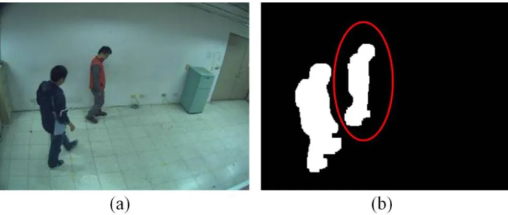
Figure 1.2 An example of serious occlusion in frame 215. (a) The frame shows the person dressed in red jacket is occluded. (b) The binary foreground image of (a).
background subtraction. With difference of 30 frames between the two figures, the circled
foreground region in Figure 1.1(b) can be clearly recognized as an isolated person, but it is
hard to distinguish the region in Figure 1.2(b) as two people due to the serious occlusion.
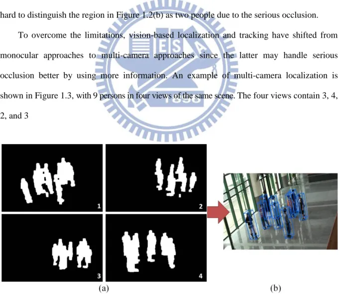
To overcome the limitations, vision-based localization and tracking have shifted from
monocular approaches to multi-camera approaches since the latter may handle serious
occlusion better by using more information. An example of multi-camera localization is
shown in Figure 1.3, with 9 persons in four views of the same scene. The four views contain 3, 4,
2, and 3
Figure 1.3 Multi-camera approach provides sufficient information for people localization. (a) The binary foreground images from four views of the same scene. (b) The localization result
3 obtained from (a) by using our method.
foreground regions with serious occlusion, respectively. But by using multiple views of the
same scene, the localization recovers information that might be missing in a particular view
and achieves good results under serious occlusion as shown in Figure 1.3(b).
However, multi-camera approach increases the amount of information from additional
views and leads to much higher computational complexity. Our purpose is to propose an
efficient and effective approach for people localization using multiple cameras, which can
handle serious occlusion in a crowd scene and provide real-time performance without special
hardware.
1.2 Review of Related Works
In the last decade, a considerable amount of approaches for people localization and
tracking have been dedicated to effectively dealing with occlusion problem. Traditional
single-camera-based monocular approaches [1]–[3] for people localization often cannot
achieve high accuracy due to the limited viewpoint and cluttering issue, i.e., a person in one
view might be partially or completely occluded by other people. To overcome these
limitations, many latest people localization schemes adopt multiple cameras [4]–[9].
Hu et al. [4] propose a method using people axes, wherein each person is represented by
an axis, to estimate the feet points in images. Before the determination of the principal axes of
people, the foreground regions need to be predefined for an isolated person, a group of people
or occluded people. Since the principal axis-based method highly relies on the accuracy of
object classification step which distinguishes the three situations of foreground regions, this
approach may not work well for dense crowd.
Instead of using shape cues or color models to analyze foreground regions in [4], Khan et
4
camera or camera pairs. The proposed method projects and integrates foreground likelihood
information of all image pixels, which is captured from different views, on multiple reference
planes of different heights to form an occupancy probability. Different from the method in [5],
which performs the reconstruction in three dimensions, the methods proposed by Fleuret et al.
[6] and Alahi et al. [7] only use the occupancy map on grids of the ground plane, which is
measured by back-projecting a predefined model, e.g., a rectangle, to image planes for
occupancy computation. Without correspondences of people between different views,
approaches presented in [5]–[7], which have high complexity in computation due to the
pixel-based processing, perform quite well under serious occlusions. However, such methods
are not suitable for certain surveillance applications, such as intruder detection and abnormal
behavior detection wherein people localization is only part of the complete process, which
need prompt attention and demand for very high processing and response speed.
In [9], Lo and Chuang propose an efficient vanishing point-based line sampling
technique for people localization with near real time performance to avoid projecting all
foreground pixels of multiple camera views to all reference planes. The computational
complexity is reduced from pixel-based to line-based processing. Multi-plane homography is
used to obtain pairwise intersections of the line samples at different heights. Then the vertical
line samples in the 3D scene can be reconstructed for people location estimation.
In this study, we continue to use the vanishing point-based line sampling technique in [9].
The efficiency of the above line sample-based approach is further improved in our method.
Without multi-plane projection for reconstruction in three dimensions, we consider only one
reference (ground) plane to analyze footsteps of people, resulting in significant improvement
in computational efficiency. Experimental results show that comparable accuracy in people
localization can be achieved with ten times in computing speed compared with our previous
5
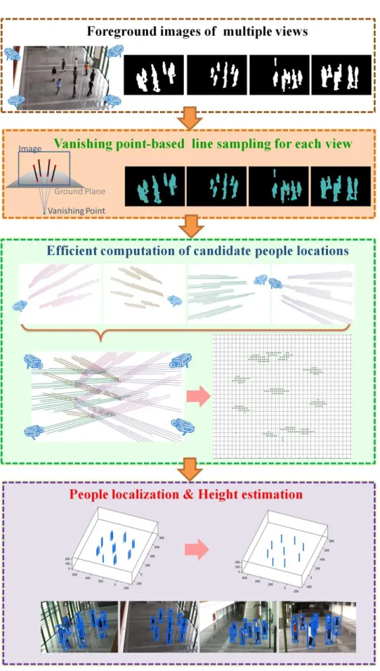
1.3 Overview of Proposed Methods
In this study, we propose an efficient and effective approach for people localization
using multiple cameras. Figure 1.4 illustrates the schematic diagram of the proposed
framework. First, the preprocessing procedure of camera calibration is executed to find the
vanishing point of vertical lines in the scene for each image plane. Next, we generate lines
originated from such a vanishing point to sample the foreground objects (people) in each
camera view, as in [9]. The line samples of foreground objects from all camera views are then
projected onto the ground plane via homographic transformation, with regions crossed
through by a large number of projected sample lines identified as candidate people locations.
We then generate (vertical) 3D line samples for these candidate people locations. After a
refinement/verification procedure for these 3D line samples, the height of each person can
also be estimated. Finally, the remaining 3D line samples are clustered into individual axes to
6
7
1.4 Contributions of This Thesis
In this study, we propose an efficient and effective method capable of locating a crowd
of dense people in real time, using multiple cameras. We retain the advantage of vanishing
point-based line sampling proposed in [9]; foreground features such as color models or shape
cues are not needed. Furthermore, we develop a 3D line sampling scheme for a single
reference ground plane to estimate people locations, instead of performing reconstruction via
computing pairwise intersections of the sample lines at different heights as in [9]. The
computational efficiency of the proposed method achieves up to 180 frames per second. For
intruder detection and abnormal behavior detection to function properly wherein people
localization is only part of the complete process, our approach may help to provide prompt
attention with very high processing and response speed. Experiments show satisfactory recall
and precision rates can be achieved by the proposed method under serious occlusion for some
crowded scenes in the real world.
1.5 Thesis Organization
The remainder of this thesis is organized as follows. In Chapter 2, we explain how to
generate 2D line samples in multi-view based on vanishing points. In Chapter 3, a two-layer
grid occupancy map is generated by projecting the above 2D line samples on ground for
footstep analysis which estimates candidate people locations. In Chapter 4, 3D line samples
are generated from these candidate people locations. Refinement/verification scheme is then
developed to validate each 3D line sample. Experimental results with reasonable performance
in people localization in terms of accuracy and efficiency are given in Chapter 5. Finally,
8
Chapter 2. Vanishing Point-Based Line
Sampling and Projection
In this chapter, we will review the process developed in [9] for generating line samples
of foreground regions in 2D views, before they are projected to the reference ground plane for
subsequent people localization process proposed in this thesis. In Section 2.1, the generation
of line samples in 2D views based on the vanishing points where vertical lines in 3D space
converge is reviewed. The estimation of these vanishing points and the 2D line-based
sampling are also presented. In Section 2.2, after the 2D foreground line samples are created,
we describe how to project them to the ground plane via homographic transformation. Figure
2.1 shows the process of vanishing point-based line sampling and projection. The projected
2D foreground line samples on the ground will be used for subsequent people occupancy
estimation.
Foreground image sequence from each view i
Vanishing point pv estimation
Vanishing point-based 2D line sample generation
Ground plane homography Hi π estimation
Projection of 2D foreground line sample to the ground
Figure 2.1 Overview of the vanishing point-based line sampling and projection
2.1 2D Line-Based Sampling from Vanishing Points
Based on projective geometry, lines in a 2D image which are parallel in the 3D space
will intersect in the 2D image at one point known as the vanishing point. Since people
walking and standing are generally perpendicular to the ground, we use the above
9
Figure 2.2 Vertical poles on the ground plane intersect in the image at the vanishing point.
In our study, we first obtain the vanishing point in each view by placing four vertical
poles on the ground plane, as shown in Figure 2.2. The linear equations of the four line
segments in the 2D image, L1, L2, L3 and L4, are obtained by detecting the red marks of the
vertical poles displayed on the image. Assume the equations are in the following form,
{ (1)
By extending the line segments of vertical poles in the 2D image, the intersection (x, y)
known as vanishing point can be found. The simultaneous equations in (1) can also be
formulated using matrices as
[ ] [ ] [ ]. (2)
To obtain the position ⃑⃑⃑⃑ of the vanishing point, we can rewrite (2) as
⃑⃑⃑⃑ , (3)
10
approximate least square solution ⃑⃑⃑⃑ can be solved by
⃑⃑⃑ , (4)
where is the pseudoinverse matrix of . It can be computed by using the singular value decomposition (SVD) of .
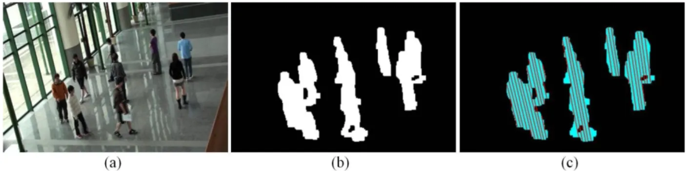
We next generate 2D foreground line samples in the associated camera view which are
originated from the vanishing point ⃑⃑⃑⃑ and correspond to a sheet of vertical 3D lines in the scene (see Figure 2.3). Line samples which do not contain enough foreground pixels will be
discarded since they are expected to be near the margin of foreground regions and will have
little contribution to 3D localization (see Figure 2.3(c)). For those line samples containing
enough pixels, they should also tolerate small areas of holes and shadows generated in
background subtraction. Such a line sampling method reduces the computational time for
analyzing the foreground information and scales down the computational complexity by
converting the underlying pixel-based processes to line-based processes. In contrast to the
principal axis-based method of finding the representation of a person proposed in [4], by
adopting the 2D line-based sampling using vanishing point, no additional foreground analysis
is required for people localization.
Figure 2.3 The 2D line-based sampling from vanishing point. (a) The original image of one view. (b) Foreground image of (a). (c) Vanishing point-originated line samples for (b).
11
2.2 Line Projection via Ground Plane Homography
Since people walking and standing are generally perpendicular to the ground and the 2D
foreground line samples correspond to vertical lines in 3D space, the projected foreground
line samples on the ground plane will give us the information closely related to people
locations. In this section, the 2D foreground line samples in each camera view are projected
onto the ground plane via ground plane homography.
Planar homography, the projective geometry constraint, is a non-singular linear
relationship between points on planes. Images of points on a plane in one view are related
to corresponding image points in another view by a planar homography matrix based
on homogeneous representation. Let ⃑⃑⃑ and ⃑⃑⃑ be homogeneous vectors of size 3 × 1, ⃑⃑⃑ be a point on plane and ⃑⃑⃑ be the corresponding point on plane . The two points can be associated with the 3 × 3 homographic matrix :
⃑⃑⃑ ⃑⃑⃑⃑ , (5)
where is a non-singular matrix transforming points on to points on . The
homographic matrix induced by a plane is unique up to a scale factor and is determined by 8 degrees of freedom. It can be estimated from four corresponding points in
two views [12].
12
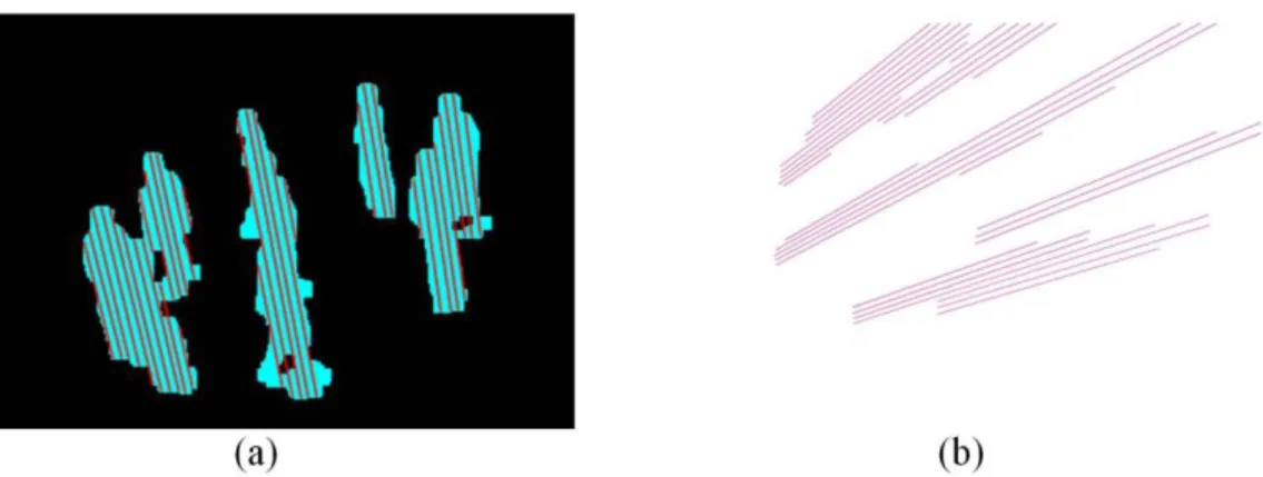
Figure 2.5 The 2D foreground line samples on image projected on ground. (a) Vanishing point-originated line samples in an image. (b) The projected 2D foreground line samples on the ground plane (top view).
In our study, we obtain in advance the positions of four landmarks , , and
on the image plane and on the ground (see Figure 2.2). Each matching pair gives two constraints and fixes two degrees of freedom, thus the ground plane homography can be obtained with four pairs of matched points. The geometrical relationship of a vertical line
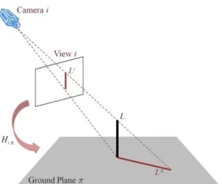
projected on ground is illustrated in Figure 2.4. Let denote a vertical line in 3D space perpendicular to the ground plane , and be the corresponding line on view i. We can obtain the projection by transforming from image plane i to ground plane π through
the homography matrix , which can be acquired by using landmarks on the ground. An
example of 2D foreground line samples projected from image to ground plane is shown in
Figure 2.5.
According to Section 2.1, the 2D foreground line samples originated from the vanishing
point can be generated to sample the foreground objects (people) in each camera view. The
line samples are then projected onto the ground plane via ground plane homography .
Figure 2.6 shows the 2D foreground line samples and the projected 2D foreground line
samples on ground in each view. As shown in Figure 2.6(d) with actual people locations
shown as red points, it is easy to see that the more a region is crossed through by the projected
13
regions which are crossed through by a large number of projected line samples as candidate
people regions.
While distal ends of the line samples shown in Figure 2.6(d) seem to be useless and can
be removed before the above process, they may contain indispensable information when
occlusion occurs. For example, the occlusion in view 2 of Figure 2.6 merges three people into
one (the largest) foreground region. To guarantee the projected 2D foreground line samples of
this region cover the actual people locations, the removable part is less than one third for all
line samples and practically irremovable for some of them. Since there are various situations
of occlusion in a crowded scene, it is hard to determine which part is removable for each line
sample. Therefore, the current practice is to retain the integrity of the projected line samples
14 (a)
(b)
(c)
(d)
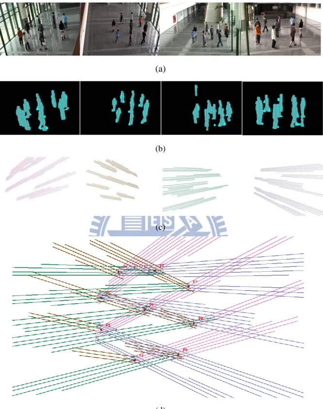
Figure 2.6 An example of projecting 2D line samples from different views onto the ground plane. (a) Original images of multiple views. (b) Vanishing point-originated 2D foreground line samples for (a). (c) The projected 2D foreground line samples on ground plane for each view (top view). (d) The 2D foreground line samples from all camera views (the union of (c)). The actual people locations are shown as red points.
15
Chapter 3. Grid-Based Estimation of
Candidate People Locations via Footstep
Analysis
In this chapter, a novel way of estimating the candidate people regions on ground by
using the projected 2D foreground line samples obtained in Chapter 2 is described. Different
from reconstructing 3D line samples to find candidate people regions, as in [9], we develop a
line sampling scheme via footstep analysis on a single reference (ground) plane to first
estimate potential people locations. As shown in Figure 2.6(d), people are more likely to stay
in regions crossed through by a large number of projected 2D foreground line samples from
all camera views. This characteristic is utilized here to estimate the candidate people regions.
In Section 3.1, we use a discretized occupancy map in which the visible part of the ground
plane is discretized into a finite number of regular blocks, and for each block the number of
crossing line samples is counted. In Section 3.2, for the blocks with enough line samples, we
then perform further screening for pre-selected locations in each block, verifying against 2D
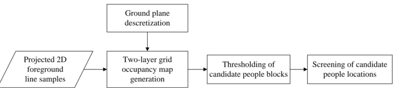
foreground images, to filter out unoccupied locations. Figure 3.1 shows the process of
grid-based estimation of candidate people locations. The retaining candidate people locations
will be further used for people localization.
Ground plane descretization Projected 2D foreground line samples Two-layer grid occupancy map generation Thresholding of candidate people blocks
Screening of candidate people locations
16
3.1 Grid-Based Discretization on Ground Plane
The main idea of this section is to acquire the distribution of people footsteps from all
camera views to find the regions where people are more likely to stay. First, we discretize the
ground plane into blocks; each block has the size of 50cm 50cm, about the area a standing person occupies. Then the number of projected 2D foreground line samples crossing each
block is counted. We next use the counted numbers to find the blocks with high densities of
crossing lines.
The process of line counting is illustrated in Figure 3.2. The line count of each block
crossed by ̅̅̅ will be increased by one. After the line counting process for each line sample from all views is completed, we obtain the discretized grid with counted numbers for the
ground plane, as shown in Figure 3.3 for the example shown in Figure 2.6. However, when
using only one descretized grid, the above line counts may distribute across neighboring
blocks. Thus we add a second grid with an offset of 25cm in both vertical and horizontal
directions from the first one. Figure 3.4 shows the result of the line counting for second grid
for the example in Figure 2.6, with the spatial relation between the two grids shown in Figure
3.5.
17
Figure 3.3 Result of the line counting for the first grid (layer 1) on the ground plane for the example shown in Figure 2.6. The numbers in each block represents the quantity of line samples crossing though it.
Figure 3.4 Result of the line counting for the second grid (layer 2) on the ground plane for the example shown in Figure 2.6.
18
Figure 3.5 Two grids with an offset of 25cm in both vertical and horizontal directions.
Note that some blocks in one grid may have higher counts than the other grid with an
offset. As shown in Figure 3.6, the line sample count dispersed by neighboring blocks can be
compensated by using two grids with an offset. In Figure 3.6(a), the line count in the blue
circled region is distributed over 4 blocks in layer 1, but is more concentrated in layer 2 with
the largest number of line samples equal to 16. On the other hand, in Figure 3.6(b), the line
count in the red circled region is more concentrated in layer 1 with the largest number of line
samples equal to 13, but is distributed over 4 blocks in layer 2.
After all blocks have been counted, we obtain the two-layer grid occupancy map as
shown in Figure 3.7. We then merge the overlapping grids into a quarter size grid. The higher
count is retained for each quarter block, as illustrated in Figure 3.8.
Figure 3.6 Close-up views of portions of Figure 3.3and Figure 3.4showing some line counts are dispersed among neighboring blocks. (a) The line count in the blue circled region is distributed in layer 1 (on the left), but is more concentrated in layer 2 (on the right). (b) The line count in the red circled region is more concentrated in layer 1, but is distributed in layer 2.
19
Figure 3.7 The two-layer grid occupancy map obtained by combining two grids (shown in Figure 3.3and Figure 3.4).
Figure 3.8 The two-layered grids are merged into a quarter size grid by retaining the one with higher count.
3.2 Candidate People Locations Estimation
By examining the two-layer grid occupancy map, numbers shown in the quarter blocks
which count the projected 2D foreground line samples from all camera views seem to
represent the distribution of people footsteps reasonably. Accordingly, the main purpose of
this section is to reduce the number of regions need to be verified further to see whether they
are occupied by persons. The determination of which quarter blocks should be retained as
20
● The quarter blocks whose counts are greater than a threshold Tc are identified as
candidate people blocks (CPBs).
● The CPBs are then filtered by a single-plane screening, at leg level hl, to find the
most likely candidate people locations (CPLs).
We first use a thresholding process to find the dense blocks from the two-layer grid
occupancy map. The CPBs are those quarter blocks whose counts are greater than a threshold
Tc. We set Tc = 8, which requires that a CPB is crossed through by sample lines from at least
two camera views. The quarter blocks after thresholding are shown in Figure 3.9.
Figure 3.9 The candidate people blocks (CPBs) for the example shown in Figure 3.7.
After the CPBs have been obtained with the above thresholding, four sample points are
generated from each quarter block region, as shown in Figure 3.10, for the preparation of
single-plane screening, which is based on point transformation via homography. The sample
points generated from CPBs are shown in Figure 3.11. Here we generate four regular points
21
one another. For example, if only one point, e.g., the block center, is generated from each
CPB, then the CPB with size 25cm 25cm can only have a maximum of one person identified in the 25cm 25cm region.
Figure 3.10 The illustration of generating four sample points in each CPB.
Figure 3.11 Sample points for the CPBs shown in Figure 3.9.
After the sample points are generated from CPBs, we then apply the single-plane
screening to remove inconsistent positions produced in CPBs. We first set an altitude hl at
human leg level, which is defined as 50cm. And we use the homography matrix Hli to
transform points on plane at hl to image view i. In particular, let P0 = (x, y, 0) be one of the
points in a CPB. Suppose a person is standing at position P0, then image of point Pl =(x, y, hl)
projected to any camera view should stay inside his/her leg region and covered by some
22
point Pl at the leg level to view i. The point P0 in a CPB region will be discarded if there exist
an i such that the above projection does not satisfy the above constraint.
Figure 3.12 Projecting point at leg level hl to image view i.
Figure 3.13 shows the remaining points, called the candidate people locations (CPLs),
obtained after the above screening process for the example shown in Figure 3.11. These CPLs
which is substantially reduced from original sample points in the CPBs will be used further
for following chapter for finding people locations.
23
Chapter 4. People Localization and Height
Estimation
In this chapter, we describe how to achieve the goal of people localization and height
estimation based on the 2D candidate people locations (CPLs) obtained in Chapter 3. In
Section 4.1, 3D vertical line samples of human body with a pre-set height h are generated.
These 3D line samples are refined with respect to foreground images from different views.
The people heights in the 3D space are then estimated by using the view-invariant cross ratio.
In Section 4.2, the refined 3D line samples are screened by some physical properties of human
body and a foreground coverage rate from different views. After the above verification
procedures, those retained 3D line samples are clustered into axes of individual persons by
using the breadth-first search (BFS). Figure 4.1 shows the process of 3D people localization
and height estimation.
Candidate people locations on ground
Generation of 3D line samples
Refinement of 3D line samples and height estimation
Clustering of qualified 3D line samples
Estimated people locations
and heights
Figure 4.1 Overview of 3D people localization and height estimation
4.1 Refinement of 3D Line Samples
In this section, we show how to form 3D line samples of human body in the 3D space.
We first establish an initial 3D line sample with a pre-set height h on each CPL. The height h,
which is set to be 200cm, should be a value higher than a normal human height. After that,
these initial 3D line samples are then refined against foreground images.
24
in the scene, its image in all views should be covered by foreground regions. In other words,
its top and bottom end points will be covered by foreground regions in all views. If that is not
the case, the initial 3D line sample should be shortened until it falls within foreground regions
in all views. As shown in Figure 4.2, assume the coordinate of the CPL is (x, y) on the ground
plane, and the top of the initial 3D line sample is Ph = (x, y, 200). The height of an initial 3D
line sample will be shortened to a reasonable length to fit the real height of a person in view i
can be achieved by
● Project the top and bottom end points, Ph and P0, of the initial 3D line sample onto
camera view i as phi and p0i, respectively.
● Move phi and p0i inward until they are covered by a foreground region.
As shown in Figure 4.2, the back projections from ground plane π and pre-set height plane πh
to the image plane view i are via the homagraphic matrixes H0i and Hhi respectively.
25
Figure 4.3 An example of 2D refinement in each camera view i with one observed person. (a) The initial 3D line samples (red) and the refined ones (blue) in the binary foreground images of all views. (b) The initial 3D line samples (red) and the refined ones (blue) in the original images of all views.
Consider the example shown in Figure 4.3 wherein the initial 3D line sample located on
one CPL is projected onto each camera view. For easy observation of the refinement result,
we only show one line sample of an observed person. The projected line samples with 200cm
height in 3D space are shown in red, with the refined portions shown in blue. Note that both
the top and bottom of the refined line samples must be covered by foreground regions.
After the 2D refinement in each camera view, we can efficiently estimate the 3D human
heights by using cross ratio. Cross ratio is a ratio of distances associated with an ordered
quadruple of collinear points preserved under projective geometry. Given four collinear points
A, B, C and D, one definition of the cross ratio used in our method is given by
̅̅̅̅ ̅̅̅̅ ̅̅̅̅̅̅̅̅. (6) The ratio CR of these distances is invariant under projective transformations. As shown in
Figure 4.4, the four collinear points A, B, C and D are related to collinear points A’, B’, C’ and
D’ by a projective transformation. Thus the cross ratio CR’ is equal to the cross ratio CR:
26
Figure 4.4 The cross ratios CR(A, B, C, D) and CR’(A’, B’, C’, D’) are equal, since points A, B,
C, D and A', B', C', D' are related by a projective transformation.
To estimate the height of the refined 3D top point (see Figure 4.2), we can utilize the collinear points, phi, pti, p0i and pvi, obtained in the 2D view i, as illustrated in
Figure 4.5. In particular, consider the cross ratio CRti (phi, pti, p0i, pvi) in view i given by
( ) ̅̅̅̅̅̅̅ ̅̅̅̅̅̅̅ ̅̅̅̅̅̅̅̅̅̅̅̅̅̅. (8)
Figure 4.5 The relationship of the collinear points on 2D view i. (Please refer to Figure 4.2 for detailed relation between the 3D line sample and the projected one on image view i.)
Note that the fourth point is the vanishing point , which is mentioned in Chapter 2. And the
refined bottom point pbi has not yet been used since we are finding the height of the top
point Pti of the 3D line sample. From (7), we know that the cross ratio CRti in view i is equal
to the cross ratio CRti in the 3D space, or
̅̅̅̅̅̅̅ ̅̅̅̅̅̅̅ ̅̅̅̅̅̅̅̅̅̅̅̅̅̅ ̅̅̅̅̅̅̅̅ ̅̅̅̅̅̅̅
27
Since Pv is approach infinity in the 3D space, the distances from points Pv to others will
approach ∞, then ̅̅̅̅̅̅ is the only unknown value in (9) and we can get
(10)
where ̅̅̅̅̅̅ is the pre-set height of the initial 3D line sample. Similarly, the refined 3D bottom point height (see Figure 4.2) can be obtained as
(11)
where utilize the collinear points phi, pbi, p0i and pvi obtained in 2D view i. Note that the
refined 2D bottom point pbi is used to substitute for the top point pti. For error tolerance, e.g.,
to cope with noises and occlusion, the intersection of all the refined 3D line samples from
different camera views is adopted as the final 3D line sample of a possible human body for
each CPL. Thus, the heights and of two end points Pt and Pb of the final 3D line
sample for each CPL is given by
, (12)
. (13)
Consider Figure 4.3 for an occlusion example, the projected 3D line sample in view 2 is
projected onto an occlusion region, and the line sample in this view cannot be refined to a
proper height; thus we further apply the intersection of all the refined 3D line samples to cope
with occlusion in 2D views.
4.2 Generation of Major Axes of People
After the 3D line samples with the refined top and bottom points Pt and Pb for each CPLs
have been obtained, we need to further verify whether the refined 3D line samples correspond
to a person existing in the 3D scene. The following procedures are the same as adopted in [9].
28 human body based on the following two conditions:
(a) Length constraint: the length of a 3D line sample is longer than the length threshold
THlen, i.e.,
̅̅̅̅̅̅ > 𝑇 𝑙𝑒𝑛. (14)
(b) Foot height constraint: the height of its bottom end point Pb does not exceed the
bottom-position threshold THbot, i.e.,
< 𝑇 𝑜 . (15)
The thresholds THlen and THbot are set to be 130cm and 50cm in our approach respectively.
The main objective of the above two conditions is to preserve two kinds of 3D line samples
which correspond to (i) the full length of a standing/walking person or (ii) the torso of a
person with his/her feet. In practice, these two rules can efficiently remove most of
inappropriate 3D line samples. While the first two filtering rules listed above are more
intuitive, we now focus on the third rule to check the foreground coverage of a 3D line
sample:
(c) Average foreground coverage rate (AFCR): the foreground coverage rate in all
views of the 3D line sample is higher than a threshold THfg.
Accordingly, We back project the 3D line sample to check the foreground coverage of
different height levels. For a person do appear in the monitored scene, these back-projected
points should be covered by some foreground regions. For example, if all back-projected
points in all views for a 3D line sample are of foreground, its AFCR is equal to 100%.
After the above verification procedure (a)-(c), the major axis (MA) of a person can be estimated from the remaining 3D line samples. To that end, an undirected graph is built for
these line samples in such a way that an edge will be established for any two of them if their
horizontal distance is shorter than a threshold Tc (= 25cm). Then, we apply breadth-first
29
frame with 9 persons shown in Figure 4.6(a), and 3D line samples obtained with the above
verification procedure are shown in Figure 4.6(b). To locate individual persons, the position
of each of them can be estimated as the average position of the members in the corresponding
cluster, as shown as a blue point in Figure 4.6(c). Finally, for each cluster, a major axis (MA)
to represent the corresponding person is established at the above average position as shown in
Figure 4.6(d), with the maximum height of the members of the cluster being regarded as a
person’s height.
Figure 4.6 Clustering and localization results after refinement and verification procedures for the example in Figure 3.13. (a) Input frame (9 persons). (b) Verified 3D line samples. (c) Top view of the clustering sets with red points representing the ground truth, and blue points representing the estimations, of people locations in this scene, respectively. (d) The 3D major axes (MAs).
30
Chapter 5. Experimental Results
Our experiments are conducted for three QVGA resolution (360240) video sequences with 30 frames per second; each has four camera views of an indoor scene under different
degrees of occlusion. The calibration poles are placed vertically on the ground of the scene
beforehand, for the estimation of vanishing points, and multiple homographic matrices. These
sequences are captured with different numbers and trajectories of people. Table 5.1 shows the
detailed information for three testing sequences, named S1, S2, and S3, respectively. The
average distance between the cameras and the monitored area is about 15m. The computation
is performed with a PC under Windows 7 with 4 GB DDR3 RAM and a 2.4G Intel i5 M520
CPU, without using any additional hardware.
Table 5.1 The information of three video sequences
Sequence Number of frames Number of persons
S1 691 9
(eight circling the center one)
S2 776 9
(walking randomly)
S3 271 12
(walking randomly)
Figure 5.1(a) shows an example frame of sequence S1. One can see that the lighting
conditions are quite complicated. The sun light may come through the windows directly and the reflections from the floor can be seen clearly. A total of 691 frames are captured for S1 wherein eight persons are walking periodically around the ninth one standing near the center
of the monitored area. Figure 5.1(b) and (c) show the verified 3D line samples and the MAs to
31
easily correspond to camera view 1 (the left most one in Figure 5.1(a)). In addition, for a
closer examination of the correctness of the proposed people localization and the height
estimation scheme, bounding boxes with a fixed cross-section of 50cm × 50cm, and with their
heights obtained, are back-projected to the captured images, as shown in Figure 5.1(d). One
can see that these bounding boxes do overlay nicely with the corresponding individuals. The
recall and precision rates for the whole sequence are evaluated as 95.8% and 95.7%,
respectively.
Figure 5.1 An instance of sequence S1, frame 1 (9 persons, eight circling the center one). (a) Input frame from four different viewing directions. (b) Verified 3D line samples of different clusters in the scene. (c) 3D major axes (MAs) to represent different persons in the scene. (d) Localization results illustrated with bounding boxes.
32
Figure 5.2(a) shows an instance of sequence S2, which has the same people count as that
for S1, but the nine people are walking randomly in the scene. While S2 may have more
serious occlusions in some time intervals, the repeated occlusions caused by periodic walking
pattern in S1 do not occur in S2. As a result, both the average recall and precision rates are
increased slightly. To further examine the robustness of our method under serious occlusion,
sequence S3 is evaluated, which is similar to S2 but having twelve persons randomly walking
in the scene. While satisfactory localization results are obtained in Figures 5.3, the recall and
precision rates for S3 are decreased to 92.9% and 91.2%, respectively. As the localization
results of above sequences summarized in Table 5.2, the proposed approach seems to work
robustly despite some degradation in localization accuracy for serious occlusion.
33
Figure 5.3 An instance of sequence S3, frame 1 (12 persons, walking randomly).
Table 5.2 Performance of the proposed approach
Sequence Recall Precision Average error FPS
S1 95.8% 95.7% 11.86cm 236.36
S2 96.2% 96.2% 10.57cm 231.62
S3 92.9% 91.2% 11.25cm 181.96
In our experiments, the “Recall” and “Precision” are defined by
𝑜 𝑒 𝑒 𝑒 𝑜𝑛 𝑜 𝑒 , (16)
𝑜 𝑒 𝑙 𝑒 𝑙 𝑜 𝑒 . (17)
An estimated location at a distance less than 30cm from the ground truth is regarded as correct, and the “Average error” gives the average distance between the estimated people
34
locations and those of ground truth produced manually. The precision and recall rates in all
the three videos are above 90%. The computational speed, in frames per second (FPS), are
evaluated without including the cost of background subtraction. The proposed approach
achieves very high computational efficiency, even for the crowded scene S3, wherein 12
persons can be located quite accurately at a high processing speed of about 180 fps. The FPS
degradation in S3 is because the computational time is dominated by the number of 2D line
samples, which will grow with the area of foregrounds. As for the accuracy, the average error
is lesser than 12cm, respectively, which can hopefully be regarded as sufficient for many
surveillance applications
Although the above evaluations show that the proposed method can often provide
reasonably good localization results, there are extreme cases which cannot be completely
handled with the proposed method. Firstly, when the foreground regions are broken at leg
level, the initial 3D line sample will not be generated and the miss detection will occur. For
the example shown in Figure 5.4, the person with a blue shirt cannot be detected since the
broken foreground region is at his leg level and this position will not be taken as a candidate
people location (CPL). Secondly, while the scene is under very serious occlusions, e.g., in
Figure 5.5, the ground region may be covered by foreground regions in all views and a false
alarm will occur (see the circled regions in Figure 5.5(a) and (b)). No matter a person does
exist or not, a 3D line sample will be generated. If such a 3D line sample cannot be filtered
out by the aforementioned verification procedure, a false alarm will occur (see the 3D MA in
red in Figure 5.5(c)). Finally, when the distances between people are too small, their 3D MAs
will be clustered into the same group. And this will lead to two miss detections and one false
alarm, as shown in Figure 5.6. For localization efficiency, the BFS scheme for clustering only
35
Figure 5.4 An example of miss detection in sequence S2. (a) Segmented foreground regions and 2D line samples. (b) The localization results wherein the person with blue shirt cannot be detected because of the broken foreground region at his leg level.
Figure 5.5 An example of false alarms in sequence S2. (a) Segmented foreground regions and 2D line samples in all views. (b) The localization results illustrated with bounding boxes in all views. (c) The 3D MAs to represent different persons in the scene. The 3D MA in red represents a false alarm.
36
Figure 5.6 An example of miss detections and false alarms in sequence S2. (a) The localization results illustrated with bounding boxes. (b) Clusters of verified 3D line samples in the scene with the circled region indicating the merge of two clusters.
For performance comparison with previous research, similar results of people
localization obtained in [9] are listed in Table 5.3 (compared with Table 5.2). One can see that
the approach proposed in this thesis achieves similar precision and recall rates as in [9].
However, the processing speed is significantly enhanced, about ten times faster than [9], due
to the use of projected 2D foreground line samples on ground, instead of reconstructing 3D
major axes via computing pairwise intersections of sample lines of image foreground
projected at different heights.
Table 5.3 Performance of people localization of [9].
Sequence Recall Precision Avg. error FPS
S1 93.7% 95.1% 11.07 cm 26.69
S2 94.3% 94.1% 9.56 cm 26.33
37
The results of person height estimation for S1 are shown in Figure 5.7. The red squares
indicate the actual heights and blue dots represent the estimated heights together with
intervals of unit standard deviations. Figure 5.8 shows similar results of person height
estimation for S2 can be obtained. However, when the occlusion becomes more serious, the
performance of height estimation of S3 is degraded as shown in Figure 5.9. More detailed
data of people height estimation can be found in Table 5.4, Table 5.5 and Table 5.6 for S1-S3.
Figure 5.7 Results of person height estimation for S1.
Figure 5.8 Results of person height estimation for S2.
38
Table 5.4 Results of person height estimation for S1.
P1 P2 P3 P4 P5 P6 P7 P8 P9
Actual 167 166 173 170 174 171 174 180 172
Average 168.5 167.1 174.2 170.0 170.0 173.8 173.0 178.3 171.7
Std 5.3 5.1 6.6 5.6 5.7 5.3 6.5 4.9 7.6
Error 1.5 1.1 1.2 0.0 4.0 2.8 1.0 1.7 0.3
Table 5.5 Results of person height estimation for S2.
P1 P2 P3 P4 P5 P6 P7 P8 P9
Actual 170 171 180 166 174 172 167 174 173
Average 172.4 176.2 174.9 165.7 169.9 174.1 171.3 173.5 173.8
Std 4.3 5.2 5.1 5.7 6.6 6.6 6.0 5.8 3.7
Error 2.4 5.2 5.1 0.3 4.1 2.1 4.3 0.5 0.8
Table 5.6 Results of person height estimation for S3.
P1 P2 P3 P4 P5 P6 P7 P8 P9 P10 P11 P12
Actual 174 180 191 166 174 173 173 170 172 167 168 171
Average 168.9 171.4 186.8 164.3 178.7 183.9 171.9 167.9 173.8 170.4 170.8 176.1
Std 3.6 6.6 9.0 7.3 9.1 9.5 6.4 2.6 5.4 3.4 7.2 5.3
39
Chapter 6. Conclusions and Future Works
6.1 Conclusions
In this thesis, an efficient and effective approach for people localization using multiple
cameras is proposed. Instead of reconstructing 3D major axes via computing pairwise
intersections of the line samples at different heights, as in [9], we retain the advantage of
vanishing point-based line sampling, and develop a sampling scheme based on the discretized
two-layer grid occupancy map. This map is adopted to count the number of projected 2D
foreground line samples, and then be used to find out occupied locations effectively. Thus, the
computation cost is greatly reduced without sacrificing the correctness and accuracy. The
experiments, conducting on three video sequences with serious occlusions, also verify the
effectiveness and efficiency of the proposed approach. The comparable accuracy in people
localization can be achieved with ten times in computing speed compared with the previous
work [9] with high processing speed of about 180 fps. This also shows our method can be
applied for many applications that require real-time performance such as intruder detection
and abnormal behavior detection.
6.2 Future Works
We are currently working on adding tracking mechanisms, and expect to see further
reduction in average errors in people localization. The person height information can also be
contributive to the applications of user-designated video query and retrieval. Furthermore, we
expect to design an automatic adjustment method finding applicable parameters for different
40
References
[1] H.Wang, D. Suter, K. Schindler, and C. Shen, “Adaptive object tracking based on an effective appearance filter,” IEEE Trans. Pattern Analysis and Machine
Intelligence, vol. 29, no. 9, pp. 1661–1667, 2007.
[2] K. Nummiaro, E. Koller-Meier, and L. Van Gool, “An adaptive color-based particle filter,” Image and Vision Computing, vol. 21, no. 1, pp. 99–110, 2003. [3] S. M. Khan and M. Shah, “Tracking people in presence of occlusion,” in Proc.
Asian Conf. on Computer Vision, pp. 1132–1137, 2000.
[4] W. Hu, M. Hu, X. Zhou, T. Tan, J. Lou, and S. Maybank, “Principal axis-based correspondence between multiple cameras for people tracking,” IEEE Trans.
Pattern Analysis and Machine Intelligence, vol. 28, no. 4, pp. 663–671, 2006.
[5] S. M. Khan and M. Shah, “Tracking multiple occluding people by localizing on multiple scene planes,” IEEE Trans. Pattern Analysis and Machine Intelligence, vol. 31, no. 3, pp. 505–519, 2009.
[6] F. Fleuret, J. Berclaz, R. Lengagne, and P. Fua, “Multicamera people tracking with a probabilistic occupancy map,” IEEE Trans. Pattern Analysis and Machine
Intelligence, vol. 30, no. 2, pp. 267-282, 2008.
[7] A. Alahi, L. Jacques, Y. Boursier, and P. Vandergheynst, “Sparsity driven people localization with a heterogeneous network of cameras,” Journal of Mathematical
Imaging and Vision, vol.41, no. 1, pp. 39–58, 2011.
[8] M. Liem and D. M. Gavrila, “Multi-person localization and track assignment in overlapping camera views,” Proc. 33rd Annual Symposium of the German
Association for Pattern Recognition, pp. 173–183, 2011.
[9] K. H. Lo and J. H. Chuang, “Vanishing point-based line sampling for efficient axis-based people localization,” in Proc. IEEE Int. Conf. on Image Processing, pp. 529-532, 2011.
[10] H. H. Lin, T. L. Liu and J. H. Chuang, “Learning a scene background model via classification,” IEEE Transactions on Signal Processing, vol. 57, no. 5, pp. 1641-1654, 2009.
41
[11] H. H. Lin, J. H. Chuang and T. L. Liu, “ Regularized background adaptation: a novel learning rate control scheme for gaussian mixture modeling,” IEEE
Transactions on Image Processing, vol. 20, no. 3, pp. 822-836, Mar. 2011.
[12] A. Agarwal, C. V. Jawahar, and P. J. Narayanan, “A survey of planar homography estimation techniques,” Technical report, IIT-Hyderabad, 2005.
[13] S. M. Khan and M. Shah, “A multi-view approach to tracking people in crowded scenes using a planar homography constraint,” Proc. Ninth European Conf.
Computer Vision, 2006.
[14] R. Eshel and Y. Moses, "Homography based multiple camera detection and tracking of people in a dense Crowd," IEEE Conference on Computer Vision and