感知雲端網路中具服務品質的資源分配

國

立

交

通

大

學

資訊科學與工程研究所

碩

士

論

文

感 知 雲 端 網 路 中 具 服 務 品 質 支 援 的 資 源 分 配

Resource Allocation with QoS Support in Cognitive Radio Cloud

Network

研 究 生：梁喬峰

指導教授：趙禧綠 教授

感知雲端網路中具服務品質支援的資源分配

Resource Allocation with QoS Support in Cognitive Radio Cloud Network

研 究 生：梁喬峰 Student：Chiau-Feng Liang

指導教授：趙禧綠 Advisor：Hsi-Lu Chao

國 立 交 通 大 學

資 訊 工 程 與 科 學 研 究 所

碩 士 論 文

A Thesis

Submitted to Institute of Computer Science and Engineering College of Computer Science

National Chiao Tung University in partial Fulfillment of the Requirements

for the Degree of Master

in

Computer Science

October 2012

Hsinchu, Taiwan, Republic of China

I

摘要

近年來，在感知無線電網路(cognitive radio network)中的資源分配持續受到高度關注。 在之前的論文中，我們設計了一個運作在電視空白頻譜(TV white space)上的感知無線電 雲端網路。為了有效利用電視空白頻譜的資源，我們提出了一個適用於我們系統上的資 源管理架構。我們的資源管理架構主要分成三個部分，包括在雲端上的分群及資源管理、 在雲端上的功率控制及資源分配、以及在感知無線電存取點上的資源管理。這篇論文中， 我們集中在第三部分。具體來說，我們將使用者分成幾個群組、定義一些服務類別、並 將使用者的需求轉換成所需頻道數。再雲端完成資源管理前兩層的資源分配及功率控制 後，我們設計的演算法將進一步以時間區塊為單位分配資源給感知無線電使用者，並最 大化系統的效能。 為了有效率地解決這個問題，我們提出了一個貪婪搜尋演算法，且這個演算化找出 的解幾乎近似於最佳解。除此之外，我們提出了優先權參數來達到相同服務類別之使用 者之間的公平性。最後，從模擬結果中可以看出，不論在效能上，或是同服務類別的使 用者之間的公平性，我們提出的演算法都能產生出色的成果。

II

Abstract

Resource allocation in cognitive radio (CR) networks is highly concerned in recent years. We have designed cognitive radio cloud network (CRCN) in TV white space in previous works. To effectively use the resource, we proposed a resource management scheme for our CRCN. Our resource management scheme is separated to three parts, clustering and resource management in Cloud, power control and channel allocation in Cloud, and resource management in CR access points (CRAPs). This paper focuses on the third part. Specifically, we first allocate users to several groups, define several service classes, and map users’ requests to the numbers of required channels. After the first two-tiers channel allocation and power control mechanisms performed at the Cloud,the designed scheduling algorithm further allocates resources (in terms of time slots) to CR users to maximize the sum of throughout utilities.

To solve the problem efficiently, we proposed a greedy search algorithm, and the scheduling results are almost close to optimal solutions. In addition, we proposed a priority factor to achieve the inner-class fairness even upon low channel availability. Finally, the simulation results show that no matter in throughput or inner-class fairness, our proposed algorithms can yield excellent results.

III

致謝

從進入研究所到現在已經經過了兩年，在這兩年間歷經了許多困難與挫折，也獲得 了許多喜悅與成就。一路走到這裡，很高興能夠完成課業和論文，為未來打下基石。 首先，感謝家人對我的支持與照顧。從高中開始家人就支持我的興趣，讓我自己選 擇自己想走的路，並在我遇到挫折時給予鼓勵與教誨。也感謝家人在經濟上給予照顧， 讓我能無後顧之憂地完成我的學業。 接著，我想感謝我的指導老師，趙禧綠教授。從碩一開始，老師在各方面不斷要求 我，並且適時地指正我的錯誤並給予建議，讓我在就學期間，無論是處事應對、課業及 基礎技能上都能有所成長。也非常感謝老師對我的體諒與包容，在我遇到困境時，能設 身處地地為我著想，以圓融的方式來解決我遇到的問題。 除此之外，我也要感謝實驗室裡的學長姐、同學及學弟妹們。在我遇到問題時，學 長姐總是能給予充分的協助並提供建議，使我能快速地融入實驗室並步上軌道。感謝同 學與我一同度過這二年間的苦樂歡笑，遇到問題時能一起討論、解決；有快樂的事能一 同分享。很感謝他們在到法國參加 conference 的期間給予體諒與照顧，讓我留下第一 次出國的美好回憶。也謝謝學弟妹在各方面的配合及協助，讓計畫的交接得以順利進行， 他們的幫助也讓我能順利準備並完成口試。 最後，我要感謝交通大學提供這麼豐富的資源給我們。網路資源讓我能找到不論在 課業上或是研究上所需的資料；教學資源讓我能選擇自己有興趣的課題，在專業技能上 獲得成長；空間資源讓我在需要討論、休息或是運動時都能夠順利找到適合的場所。 畢業的時候來臨了。在離開校園，進入職業之後，我會將這兩年在交通大學所學到 的知識應用在工作上，期望能為這個世界的科技造詣上盡一份心力，為人類帶來更便利、 更美好的世界。在這裡，我要感謝我的家人、所有在教學上指導過我的教授們、實驗室 的學長姐、同學、學弟妹、以及在這段期間我遇見的每一個人。正因為有他們，才能造 就現在的我。謝謝各位一路上的照顧與支持。

IV

Contents

摘 要……….I Abstract ………..II 致 謝………...III Contents………IV List of Tables……….VI List of Figures………..VII Chapter 1 Introduction………...……….……….1 1.1 Background……….……1 1.2 CRCN architecture……….……….2

1.3 CRCN resource management scheme……….………5

Chapter 2 System Model and Request Mapping Method………..11

2.1 MAC frame architecture and assumptions………11

2.2 Group allocation………12

2.3 Service classes………...15

2.4 Request mapping method………17

2.5 Utility functions………18

Chapter 3 Problem Setting and Scheduling Algorithms………21

3.1 Problem setting……….21

3.1.1 Motivation……….21

3.1.2 Related work……….22

3.1.3 Problem formulation……….23

3.1.4 Quantization of utility functions………...24

3.1.5 Problem formulation with quantized utility functions………..26

3.2 Scheduling algorithms………...27

3.2.1 The optimal scheduling algorithm………27

3.2.2 The proposed scheduling algorithm………..30

Chapter 4 Performance Evaluation………36

4.1 Small scale simulation………..36

V

4.1.2 Small-scale simulation results………...38

4.2 Large-scale simulation………..42

4.2.1 Large-scale parameters and environments………..42

4.2.2 Large-scale simulation results………..44

Chapter 5 Conclusions and future work………45

VI

List of Tables

Table I Common network services………15

Table II Classified service classes………..16

Table III Request mapping method………17

Table IV The results of tier-2 allocation……….18

Table V Small-scale parameters of services types………37

Table VI Small-scale parameters of utility functions………37

Table VII Large-scale parameters of service types………42

VII

List of Figures

Figure 1 CRCN architecture……….3

Figure 2 CRCN MAC protocol………4

Figure 3 Inter-cell interference………5

Figure 4 Power controlexample………6

Figure 5 CRCN resource management scheme……….8

Figure 6 Proposed MAC frame………11

Figure 7 Group allocation………12

Figure 8 An example of convex hull………13

Figure 9 Quickhull algorithm procedures in above part……….14

Figure 10 The utility function of NRT services………19

Figure 11 The utility function of video streaming………19

Figure 12 The utility function of VoIP……….19

Figure 13 An example of available rates………..………25

Figure 14 An example of quantization…………..………25

Figure 15 An example of timeslots combinations….………27

Figure 16 The optimal search tree………28

Figure 17 An example of optimal search tree………29

Figure 18 The flow chart of greedy search……….30

Figure 19 The greedy search tree………31

Figure 20 An illustrative example – initialization………32

Figure 21 An illustrative example – greedy search tree………33

Figure 22 The MAC frame in small-scale……….36

VIII

Figure 24 The comparison of utilities with different algorithms………39 Figure 25 The utility and usability with decreasing β in first case of scenario 2………..40 Figure 26 The utility and usability with decreasing β in second case of scenario 2…….40 Figure 27 The utility with increasing γ in first case of scenario 2………41 Figure 28 The utility with increasing γ in second case of scenario 2………41 Figure 29 The utility and fairness with increasing γ………44

1

Chapter 1 Introduction

1.1 Background

In recent years, with the rapid development of wireless technologies, more and more technical products have the ability to use the wireless resource, and the new wireless communication systems, such as LTE, 4G, etc., need much more resource than old wireless systems. The requirements of wireless band become higher and higher, so under the finite wireless resource condition, how to use wireless band efficiently is a highly concerned issue. According to the investigation of Federal communications Commission (FCC) [1], the average usability of licensed spectrums is very low. To increase the usability of those spectrums, one of the resource sharing techniques, Cognitive Radio (CR) [2], which is proposed by Mitola and Gerald Q. Maguire, Jr in 1999 has been highly concerned during those years.

The resource sharing technique of CR is that secondary users (referred as cognitive radio users, CR users) can temporarily borrow unused bands owned by licensed users (referred as primary users, PUs) for communication. When PUs get back to the bands borrowed by CR users, the CR users should release the bands immediately. To implement the CR resource sharing technique, CR systems should have the ability to sense and measure the characteristics and availabilities of licensed bands, and to know which channels and how long the CR users can occupy, so spectrum sensing is one of important issues in CR systems.

Another important issue is resource management. The available resource in CR network may be changeful and fractional, so how to efficiently and effectively user the resource become difficult and challenging. If the resource management is not good enough, the CR network will become unstable.

2

are classified to two types of networks: distributed CR network, like [3], and centralized CR network, such as [4] [5]. In distributed CR networks, spectrum sensing is done by each CR user (or a CR pair). CR users sense channel respectively for several milliseconds, if the channel is still idle during the time, the CR user may operate on the channel. In centralized CR networks, the measurement of resource is done by cooperative spectrum sensing (CSS). Each CR user collect the information of several channels, and then sends them to the centralized units, such as wireless access points, base stations, etc., for resource measurement. CSS has higher accuracy and completeness than distribute spectrum sensing, but it also has higher complexity. To overcome the high complexity, in [6] [7], we combine the cloud and centralized CR network as Cognitive Radio Cloud Network (CRCN).

The CRCN is a prototype of CR systems which operate on TV White Space [8]. It contains network architecture, media access control (MAC) architecture, CSS algorithm, CR access point (CRAP) and CR user managements, messages exchange scheme, and so on. In the CRCN architecture, it can measure the available resource for each CRAP, and CR users can communicate with each other and connect to the Internet by the MAC and the network architecture. However, it doesn’t have a completed resource management scheme yet, so we want to develop our one in CRCN.

Before introduce our resource management scheme in CRCN, we will first introduce the CRCN architecture in the next section.

1.2 CRCN architecture

CRCN consists of CR Cloud, CR APs, and CR users, as Figure 1. CR users associate with nearby CR APs, and communicate with associated APs by our MAC protocol. All communications between CR users or CR users and Internet are controlled by CR APs. No matter where CR users send packets to, the packets will first be sent to one CRAP, and then

3

the CRAP forwards the packets to the destination by Ethernet. For example, when SU2 wants to send a message to SU3, SU2 will send the message to CRAP1 which he associates. Then CRAP1 forwards the message to CRAP2, which the destination user, SU3, associates, and finally CRAP2 transmits the message to SU3. However, how does CRAP1 know where SU3 is? Because all CRAPs and CR users’ information are managed by CR Cloud, when CRAP1 receives a message which destination is SU3, CRAP1 will first ask CR Cloud for SU3’s location, and then forward the message to SU3’s associated CRAP.

Figure 1 CRCN architecture from [8]

CR Cloud not only manages the CRAPs and CR users’ information, but also manages the available resource of wireless spectrum. Sensing devices (SD) periodically sense data channels, and then report the sensing results to CR Cloud by CRAPs. CR Cloud uses those results to calculate the available data channels in each area by doing CSS algorithm, and records the results in database. CRAPs periodically ask CR Cloud for available data channels,

4

and announce the information to CR users in common control channel (CCC). CR users use the available data channels for communications, and share the channels between CR users by time-divided media access (TDMA). In such CRCN architecture, CRAPs are not worried about which channels they can use. They only need to care about how they should allocate the resource to their associated CR users.

Figure 2 CRCN MAC protocol from [8]

Figure 2 is our CRCN MAC protocol. In each frame, it contain several periods. There are beacon period (BP), association period (ASP), report collection period (RCP), and resource request period (RRP) in control channel, and quiet period (QP), downlink (DL), and uplink (UL) in data channels. CR users (called secondary users, SUs, here) and SDs send join/leave messages in ASP to associate/disassociate one CRAP, and confirm their successful association/disassociation by receiving beacon in BP. If they associate successfully, their host ID (host address) will be included in join list contained in beacon. After successful association, CR users send their resource requests in RRP, and do their communication in DL and UL according to the scheduling result contained in beacon. SDs sense data channels in QP, and report the sensing result in RCP. All SUs and SDs should receiving beacon during BP in

5

control, and all communication is forbidden in QP to help SDs can collect the correct sensing results, so the data channels should be idle in BP and QP.

With the CRCN architecture and MAC protocol, CR Cloud can correctly get the sensing results from SDs, and calculate the available resource for CRAPs. CRAPs announce the available resource and scheduling result in beacon, and then CR users can successfully do their communications. However, we have not designed realistic and implementable resource managements yet. Without such resource managements, CR users can’t use the available resource efficiently and reasonably. Thus, we design a novel resource management scheme, and separate it into several tiers. We will introduce the scheme in the next section.

1.3 CRCN resource management scheme

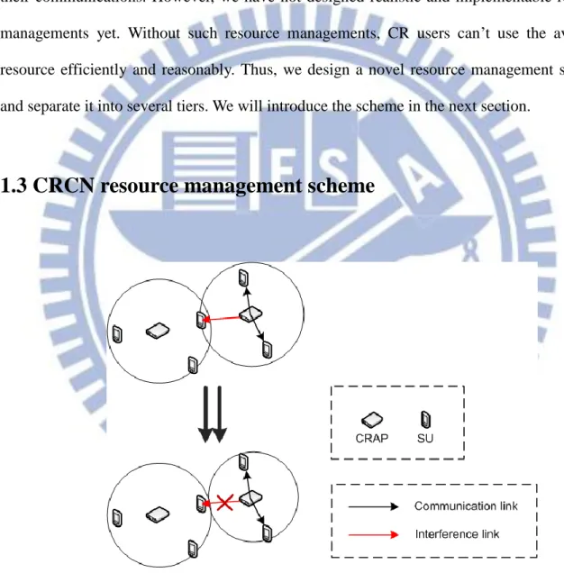
Figure 3 inter-cell interference

In our CRCN architecture, CRAPs should ask CR Cloud for available resource, they can’t decide which channels to use by themselves, so CR Cloud can manage the resource for

6

each CRAP, deciding which channels each CRAP can uses. Thus, the intuitional idea is separating the resource management into two-tiers. The first tier is from CR Cloud to CRAPs, and the second tier is from CRAPs to CR users.

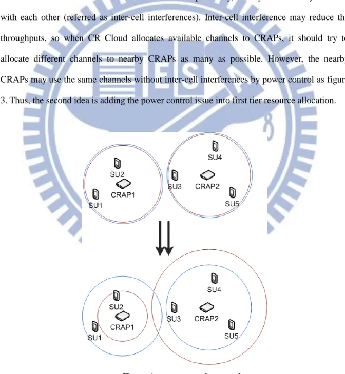
After CR Cloud calculates the available channels for CRAPs, it allocates some of these channels to each CRAP according its requirements (the amount of data it should serve), and then each CRAP use its allocated channels to serve the CR users who associate with it. Because CRAPs do their resource allocations independently, nearby CRAPs may interfere with each other (referred as inter-cell interferences). Inter-cell interference may reduce the throughputs, so when CR Cloud allocates available channels to CRAPs, it should try to allocate different channels to nearby CRAPs as many as possible. However, the nearby CRAPs may use the same channels without inter-cell interferences by power control as figure 3. Thus, the second idea is adding the power control issue into first tier resource allocation.

7

Under the second idea, the first tier allocations not only allocate available channels to each CRAP, but limit the maximal power of each channel for each CRAP, so nearby CRAPs may share the same channels, increasing the channel reusability. Nevertheless, this way is not perfect enough. For example, as figure 4, under the second idea, CRAP1 and CRAP2 share the same channels, red and blue channels, by power control. However, if CRAP1 allocated the red channel to SU2 with smaller power, and SU2 can be satisfied with the power, CRAP2 can use larger power on red channel, so CRAP2 can have higher data rate to serve its associated SUs.

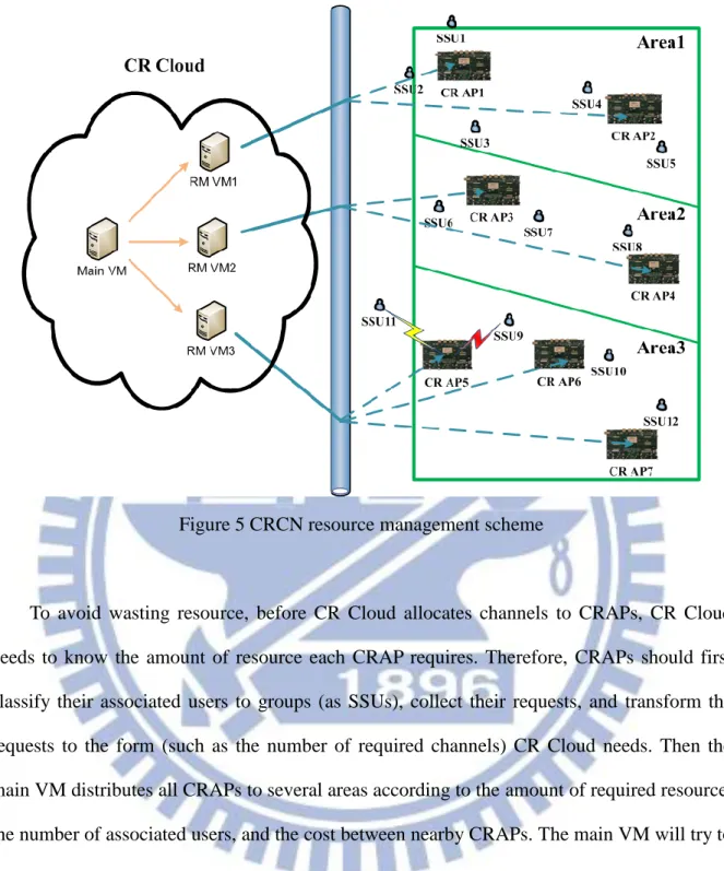
To optimize the efficiency of channels, doing power control based all users is essential. However, it is not realistic because of its high complexity. To conquer the problem, we propose a CRCN resource management scheme as Figure 5. In the scheme, we group some SUs with close locations into a super SU (referred as SSU), and then CR Cloud will only do power control based on SSUs. Also, we distribute CRAPs to several areas, and each area is controlled by one resource management virtual machine (called RM VM). Therefore, the complexity of doing power control based on SSUs can be reduced very much, so the third idea will be implementable.

In addition, because each RMVM only control one area, RMVMs can’t take the CRAPs of nearby areas into considerations, so the boundary CRAPs of nearby areas may interfere with each other. Therefore, after main VM distribute CRAPs to several areas, main VM should allocate channels to the boundary CRAPs of nearby areas first to avoid inter-cell interference as best as possible.

8

Figure 5 CRCN resource management scheme

To avoid wasting resource, before CR Cloud allocates channels to CRAPs, CR Cloud needs to know the amount of resource each CRAP requires. Therefore, CRAPs should first classify their associated users to groups (as SSUs), collect their requests, and transform the requests to the form (such as the number of required channels) CR Cloud needs. Then the main VM distributes all CRAPs to several areas according to the amount of required resource, the number of associated users, and the cost between nearby CRAPs. The main VM will try to balance the workloads of each RMVM to let each RMVM can finish their jobs under the acceptable time. In Addition, after the main VM finish areas distributing, it will allocate available channels to boundary CRAPs.

Afterwards, each RMVM will do channel allocation and power control for the CRAPs in its managed area. The channel allocation and power control will be done based on the requirement of each SSU. RMVMs allocate each SSU several channels, and limit the

9

maximum power for each channel to meet the SINR demand. RMVMs will try to satisfy each SSU’s requirements, but not absolutely, so after RMVMs finish channel allocations, SSUs may not get the whole resource they required.

Finally, CRAPs will allocate channels and timeslots to each CR users by groups. If the resource is enough, CRAPs will satisfy each CR users’ requests. But when the resource is insufficient, CRAPs need to do their scheduling based on some regulations, such as throughput, and fairness. The scheduling will be done group by group, because the power control is based on the location and requirement of each group. If CRAPs arbitrarily allocate channels to discordant groups, it will cause inter-cell interferences, reducing the throughput of CRCN.

In conclusion, the CRCN resource management scheme separates the resource allocation to three tiers. The first one is the area distribution and interference avoidance for boundary CRAPs in main VM. The second one is resource allocation and power control for CRAPs in RMVMs. And the last one is grouping, request transforming and scheduling in CRAPs.

In this paper, we will focus on the third tier, the resource management in CRAPs. There are several challenges in the third tier. At first, how should we classify CR users into groups? The definition of one group is that all CR users in the group have the same or similar SINR in a specific channel, so locations of the CR users in the same group should be close enough. However, if we classify each group in a too small range, the number of SSUs will too many, causing the complexity of power control to become too high. Therefore, the first challenge is how to define a way to classify groups by considering the two issues.

Second, after classifying groups, we should collect the request of each group, and transform it to the number of channel the CRAP needs to serve the group. Because using larger powers will have higher SINRs (data rates), CRAPs should not only tell CR Cloud how many channels they need, but also the required SINR of each channel. Hence, transforming the CR users’ request to numbers of channels with specific data rates is the second challenge.

10

At last, after CR Cloud finishes the resource allocation, CRAPs should allocate channels and timeslots to CR users group by group based on their request. If the resource is not enough, CRAPs will do scheduling based on the fairness. Because we assume each user only have one antenna, each user only can use one channel each frame. In such condition, the allocation will become a challenging problem.

The reset of this paper is organized as follows. The system models and assumptions are introduced in chapter 2, including the way to group CR users. The proposed transforming and scheduling algorithms are contained in chapter 3. The results and simulations of our algorithms are showed in chapter 4. And we summarize the conclusions in chapter 5.

11

Chapter 2 System Model and Request Mapping

Method

2.1 MAC frame architecture and assumptions

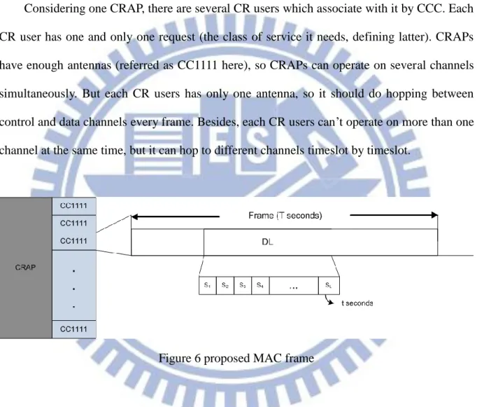
Considering one CRAP, there are several CR users which associate with it by CCC. Each CR user has one and only one request (the class of service it needs, defining latter). CRAPs have enough antennas (referred as CC1111 here), so CRAPs can operate on several channels simultaneously. But each CR users has only one antenna, so it should do hopping between control and data channels every frame. Besides, each CR users can’t operate on more than one channel at the same time, but it can hop to different channels timeslot by timeslot.

Figure 6 proposed MAC frame

The proposed MAC frame is as figure 6. The scheduling is done every frame, and we focus on the downlink allocation in this paper. Each frame has one downlink period, and each downlink period has L timeslots. The length of one timeslot is t seconds, and one frame is T seconds.

12

2.2 Group allocation

For simplicity and efficiency, we distribute users to several groups as figure 7. We allocate all users associated with the CRAP into 12 groups, by considering the distance from CRAP and the direction relative to CRAP. The two factors are quite related to the received SINR from CRAP. Under the same power, the larger distance is larger, the received SINR is smaller. In addition, the direction is related to interferences and environment block. With the same direction, the effect of interferences and environment upon received SINR will be close.

Figure 7 group allocation

Assume someone user’s location is (x, y), the CRAP’s location is (x0, y0), and the

coverage radius of CRAP is R. Also, we define two vector v0 (0, 1) and v(x- x0, y- y0). Then

we can calculate the distance between the user and CRAP and the direction from CRAP by (1), (2) and (3). 𝜃′_{= cos}−1₍𝑣o∙ 𝑣 |𝑣o||𝑣|) × 180 𝑃𝐼 (1) 𝜃 = {𝜃_{360 − 𝜃}′ , 𝑥 − 𝑥_{′ , 𝑥 − 𝑥}0 ≥ 0 0 < 0 (2)

13

𝑑 = √(𝑥 − 𝑥₀)2_{+ (𝑦 − 𝑦}

0)2 (3)

With 𝜃 and 𝑑, we can distribute the user to one of the 12 groups by formula (4)

SU ∈ 𝐺_i, 𝑖 = {⌊ 𝜃 90⌋ + 1 , 𝑑 ≤ 𝑅 2 ⌊𝜃 45⌋ + 5 , 𝑑 > 𝑅 2 (4)

After every user is allocated to one of the 12 groups, we should find a point for each group to represent the location of users who belong to the group. Assume there are M users, (𝑥1, 𝑦1), (𝑥2, 𝑦2), … , (𝑥M, 𝑦𝑀), in someone group. If M is more than 3, we will first do

quickhull algorithm [9] to find a convex hull of the M users, and then find the barycenter with those users in the apexes of the convex hull.

The definition of a convex hull is that a convex polygon consisted by several points contained in a points set can surround all points in the points set, as figure 8.

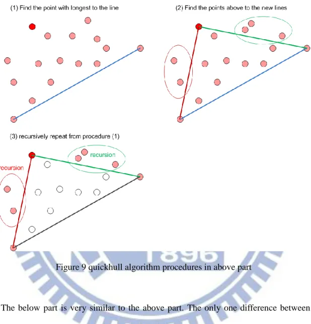
Figure 8 an example of convex hull

The quickhull is an algorithm which can find a convex hull with minimal apexes. It finds two points with longest distance first, and separates the points to two parts which are above and below to the line which link the two points. For the above part, it finds a point with longest distance to the line, and then links the new point with the two points linked by the line, so two new lines are formed. Next, it finds a new points set above to one of the new lines, and

14

recursively do the procedure with the new line and new points set until no point above to the line in current recursion.

Figure 9 quickhull algorithm procedures in above part

The below part is very similar to the above part. The only one difference between the two parts is that below part always finds the below points to the line in the current recursion. The main procedure of quickhull algorithm is conceptually showed in figure 9, and the complexity of quickhull algorithm is O(nlogn) in average cases.

After finishing quickhull algorithm, assume the convex hull is consisted by 𝑀_h points, (𝑥1, 𝑦1), (𝑥2, 𝑦2), … , (𝑥Mh, 𝑦𝑀ℎ). Then we can calculate the barycenter (𝑥c, 𝑦𝑐) by formula

15 { 𝑥_c = 1 𝑀_ℎ∑ 𝑥𝑖 𝑀ℎ 𝑖=1 𝑦c = 1 𝑀ℎ∑ 𝑦𝑖 𝑀ℎ 𝑖=1 (5)

The barycenter will represent the location of all users in the group, and it will be treated as a SSU’s coordinate in CR Cloud.

2.3 Service classes

To classify network applications to several service classes, we collect some information about common network services, and summarize them to Table I, as following.

Table I common network services

Web browsing, e-mail, telnet, and message exchanging applications, like MSN, are very common and low load services. They need less than 50K bps to keep going their services. FTP can be run on any bandwidth, but we assume that the users who use FTP are downloading large files, so low bandwidth is not suitable to FTP service. Hence, we define that FTP service needs high bandwidth to achieve a good quality of service (QoS).

16

VoIP and video streaming are real time (RT) services. Including packet headers, VoIP service needs 80K bps. If VoIP service gets bandwidth less than 80K bps, the QoS of VoIP will become rough. The bandwidth video streaming service needs varies on video qualities and encoding technology. To watch a nice video, it always needs more than 1M bps bandwidth, and as same as VoIP, the quality will seriously affected when allocated bandwidth doesn’t match its requirement.

With the above information about common network applications, we classify those applications to four service classes, as Table II.

Table II classified service classes

In the four service classes, NRT & high load services represent the NRT services which need high bandwidth, like FTP. RT & asymmetric services represent those RT services which need high bandwidth in downlink but low bandwidth in uplink. RT & symmetric service are like VoIP services which need the same bandwidth both in downlink and uplink. Finally, NRT & low load service contain all the services which needs low load service, such as web browsing, e-mail, telnet, MSN, and so on.

We assume the data rate each service class needs is 𝑅₁′, 𝑅₂′, 𝑅₃′, and 𝑅₄′, respectively, and 𝑅₁′ _{> 𝑅}

17

devices can support, and the mapped physical rate Ri should larger than 𝑅_𝑖′×𝑇

𝐿×𝑡, so one user in

ith class can be satisfied within 𝐿 timeslots (maximal number of timeslots one user can use in one frame).

2.4 Request mapping method

Before the tier-1 and tier-2 channel allocations, the Cloud must know how many resources each CRAP needs, so each CRAP have to mapping the user requests to numbers of channels

As the same assumptions in Table II, we classify users’ services to four classes, and ith class has a required data rate, 𝑅_i′, and a mapped channel quality, 𝑅_i. Considering one group, there are fi users in ith class, and we map the requests to four numbers of each mapped channel

quality with the following method, as Table III.

Channel quality

(bps) Number of channels Remaining requests

𝑅₁ 𝑁₁ = ⌊_𝑅×𝑅_×𝐿×𝑡′×𝑇⌋ 𝛿₁ = 𝑓₁𝑅₁′_{𝑇 − 𝑁} 1𝑅1𝐿𝑡 𝑅₂ 𝑁₂ = ⌊ ×𝑅_{𝑅 ×𝐿×𝑡}′×𝑇 ⌋ 𝛿₂ = 𝑓₂𝑅₂′_{𝑇 + 𝛿} 1− 𝑁2𝑅2𝐿𝑡 𝑅₃ 𝑁3 = ⌊ ×𝑅 ′_×𝑇 𝑅 ×𝐿×𝑡 ⌋ 𝛿3 = 𝑓3𝑅3 ′_{𝑇 + 𝛿} 2 − 𝑁3𝑅3𝐿𝑡 𝑅4 𝑁4 = ⌈ ×𝑅 ′_×𝑇 𝑅 ×𝐿×𝑡 ⌉

Table III request mapping method

N1 is the requested number of channels with R1 rate, N2 is the requested number of

18

𝑓𝑖× 𝑅i′× 𝑇 is the total size of data needed to send in ith class within one frame, and

𝑅_𝑖 × 𝐿 × 𝑡 is the total bits one Ri channel can transmit during downlink periods within one

frame. Hence, 𝑖×𝑅

′_×𝑇

𝑅𝑖×𝐿×𝑡 is the needed number of Ri channels to transmit all data in i

th

class. The number of channels should be an integer, so we take the floor of the value as Ni. Because

the value of 𝑁_𝑖 × 𝑅_i× 𝐿 × 𝑡 may be less than 𝑓_𝑖 × 𝑅_i′× 𝑇, so there may be some data which can’t be transmitted within Ni channels with rate Ri. Those data should be sent by followed

type of channels, so the remaining size of data will be added to the followed class. Besides, R4

is last type of rates, and we take the ceiling of the value, ×𝑅

′_×𝑇

𝑅 ×𝐿×𝑡 , as N4 to guarantee that

all of the requested data can be transmitted.

After N1 to N4 are calculated, we send the requests to CR Cloud, and wait for the results

of tier-2 allocation. The results are showed as Table IV. Because there are may not be enough channels to satisfy each CRAP’s requirements, so the results of allocated channels, 𝑁̂ to 𝑁₁ ̂, ₄ may be less than the numbers of requested channels, 𝑁₁ to 𝑁₄.

Channel Quality Number of allocated channels

R_{1 𝑁}̂ ≤ 𝑁_{1 1} R 2 𝑁̂ ≤ 𝑁2 2 R 3 𝑁̂ ≤ 𝑁3 3 R 4 𝑁̂ ≤ 𝑁4 4

Table IV the results of tier-2 allocation

2.5 Utility functions

Under such conditions, we face a challenge to do scheduling with insufficient resources. To evaluate the utility of each user under insufficient resources, we use the utility functions

19

proposed in [10], and [11] provide some ways to define the utility functions. The utility functions describe how good the service is with the allocated bandwidth (or data rate).

Different services have different utility functions, because some services have the threshold but some haven’t. Those services which have no threshold are elastic services. Elastic services can keep going even when the allocated bandwidths are very low, and they will work better when then get higher bandwidths. The elastic services are NRT services in our works, and the utility function curves of elastic services are as Figure 10.

Figure 10 the utility function of NRT services

Figure 11 and 12, the utility function of video streaming and VoIP services

Those services which have thresholds are RT services. They are almost out of going when the allocated bandwidths are under the thresholds, like VoIP services. Video streaming

20

and VoIP are RT services, but we use two different utility functions to describe the two services. We think that video streaming has more elasticity than VoIP, because video streaming services can adjust the quality of video basing on the allocated bandwidth. When the bandwidth is low, video streaming services can provide small video size to the user, and when the bandwidth is enough, it can provide the best to the user. The utility function curves of the two services are as Figure 11 and Figure 12.

The equations of the four utility functions are corresponding to the four service classes defined by formula (6) to (9), as following:

𝑈1(𝑟) = 1 − 𝑒 −𝑎 𝑟 𝑅′_{𝑇 (6)} 𝑈2(𝑟) = 1 − 𝑒− 𝑎 𝑟 𝑏 𝑟 (7) 𝑈3(𝑟) = {𝑒 𝑎 , 𝑟 𝑏 , , 𝑟 ≤ 𝑐 3 1 − 𝑒𝑎 , 𝑟 𝑏 , , 𝑟 > 𝑐₃ (8) 𝑈4(𝑟) = 1 − 𝑒 −_𝑅𝑎_′𝑟_{𝑇 (9)}

𝑈_𝑖(𝑟) is the utility function which belong to ith

class, and 𝑎_𝑖, 𝑏_𝑖, and 𝑐_𝑖 are constant values. 𝑈₁ and 𝑈₄ are utility functions of elastic services, and the values of 𝑎_𝑖 are given to decide the curvatures of the utility functions. Larger curvatures mean that the services need less bandwidth to achieve a given value of utility. We use curvatures to differentiate high load and low load in NRT services. High load services needs less percentage of their requirements to get the same value of utility than low load services, because NRT & high load services are always background downloads, and users always care about whether the downloads are keep going or not.

The scheduling under insufficient resource is our primary problem in this paper. In next chapter, we will formulate our problem with the utility functions, and introduce our proposed scheduling algorithms to solve it.

21

Chapter 3

Problem Setting and Scheduling Algorithms

In this chapter, we introduce our problem formulation to describe what scheduling problem we want to solve. Also, we introduce the optimal scheduling algorithm to solve the problem, but the complexity of optimal algorithm is too high, so it can’t be practically implemented in our system. Hence, we propose other scheduling algorithms with reasonable complexity, and we will compare the proposed algorithms and optimal algorithm in our simulations.

3.1 Problem setting

3.1.1 Motivation

In our assumption, the resources are not enough to satisfy each user’s requirement. In such case, the high priority users may be allocated more resources than low priority users. However, how to define the priorities between different services, and how much more resources should we allocate to high priority users? To define those are very difficult and indeterminate.

The core idea is that RT users have higher priority than NRT users, but it is not always true. When the resources are very insufficient, even though we allocate most of the resources to RT users, RT users still not reach their threshold. In such case, allocating no resource to RT users is better, because the services of RT users remain out of going even if we allocate resources to them. Therefore, allocating resources by considering only the priorities is not appropriate.

In such situations, the utility functions can help us to suitably define our problem. The utility of RT users will grow faster than NRT users when the allocated resources exceed the

22

threshold, so when resources are enough to serve RT users, RT users will get more resource than NRT users. Besides, when the resources are extremely insufficient, the allocated resources to RT users are hard to reach the threshold, so RT users will almost get no resource.

Thus, in our problem, the objective is to achieve the maximal summation of each user’s utility. If we achieve it, it means that we achieve the maximal throughput in our system. Moreover, we want to guarantee that (a) all users will get a minimal percentage of their requirements, and (b) the unused resources should be under a given percentage.

The minimal rates guarantee is to prevent NRT users get no resource, and the minimal rates will be decided by channel request and channel allocation result. The usability guarantee is to prevent allocating too many resources to RT users, because redundant resources are useless for RT users.

With the above consideration, we formulate our scheduling problem by utility functions in section 3.1.3.

3.1.2 Related work

Utility maximization problem is discussed many years, and finding an optimal solution is proved as a NP-Hard problem [12]. No matter whether the long-term and short-term utility optimization in routing [13] [14], or one-hop scheduling in wireless networks [11], the problem is solved many times.

However, our problem has one much different from them. In our problem, the rate is not continuous value. Because our basic scheduling unit is one timeslot and the timeslots can’t be divided, so rates are restricted by timeslots and hence they are discrete values.

Because the rates are discrete values, most of previous works are not suitable in our problem. In addition, some of works may help us to solve the problem, but they don’t have the timeslots allocation issue. Therefore, we want to design a new scheduling algorithm by considering the timeslots and utility functions to solve the problem.

23

3.1.3 Problem formulation

Notations and assumptions:

 The scheduling is done every frame

 L: number of downlink timeslots per frame  t: time of one timeslots (second)

 T: time of one frame (second)  𝑓_𝑖: number of users in ith class  𝑁̂_𝑚: number of 𝑅_𝑚 channels  𝑅_𝑖′_{: requested rate for each user in i}th

class (bits per frame, bpf)  𝑅_𝑚: rate mapped to mth class (bps)

 𝑟_𝑖,𝑗: rate allocated to jth user in ith class. (bps)

 𝑦𝑖,𝑗,𝑚: number of 𝑅𝑚 timeslots allocated to user (i,j)

The problem is formulated by equation (10) to (15).

Objective: 𝑚𝑎𝑥 (∑ ∑ 𝑖 𝑈_𝑖(𝑟_𝑖,𝑗) 𝑗=1 4 𝑖=1 ) (10) where 𝑟_𝑖,𝑗 = ∑4_𝑚=1(𝑦_{𝑖,𝑗,𝑚}× 𝑅_𝑚× 𝑡) (11) Constraints: ∑ ∑ 𝑖 𝑟_𝑖,𝑗 𝑗=1 4 𝑖=1 ≤ ∑ 𝑁̂𝑚× 𝑅𝑚× 𝐿 × 𝑡 4 𝑚=1 (12) ∀(𝑖, 𝑗), 𝑟𝑖,𝑗 𝑅_𝑖′×𝑇≥ 𝛼, 𝛼 = ∑𝑚= 𝑁̂𝑚×𝑅𝑚×𝐿×𝑡 ∑_{𝑖= 𝑖}×𝑅_𝑖′×𝑇 × 𝛾, 𝛾 < 1 (13) ∀(𝑖, 𝑗), 𝑅𝑖′×𝑇 𝑟𝑖,𝑗 ≥ 𝛽, 𝛽 < 1 (14) ∀𝑖𝑗, ∑4 𝑦_{𝑖,𝑗,𝑚} 𝑚=1 ≤ 𝐿 (15)

24

The objective is to maximize the summation of utilities, got by taking bandwidth (in our problem, called rate, bit per frame) into corresponding utility functions. The rate is calculated by the number of allocated timeslots and the rate of the channel.

There are four constraints in our problem. Equation (12) means that the summation of allocated rates shouldn’t be larger than the amount total channels can provide. Equation (13) is the minimal rate guarantee. We guarantee α percentage requirement rate to users. The α is decided by the value of _{total requirements}total resources × γ, and γ means that how many resources we want to release for minimal rate guarantee.

Equation (14) is the usability guarantee, the value of _{allocated resources}requirement should be larger

than a given value, β, and β means the minimal usability guarantee. If allocated resources are less than the requirement, the user will use all the resources, so the usability will be 1. Hence, equation (14) is meaningful only when the allocated resources are more than the requirement.

Equation (15) is to guarantee the number of allocated timeslots to any user won’t be over the number of timeslots one user can use in one frame. Each user has only one antenna, so one user can’t use more than L timeslots.

3.1.4 Quantization of utility functions

Because the rates in our system are not continuous values, we want to rewrite the utility functions by quantizing the utility functions with available rates. Because the rates is composed by types and numbers of timeslots, the available rate, r, can be calculated by equation (16) with various combination of 𝑐_𝑚.

𝑟 = ∑4 𝑐_𝑚𝑅_𝑚𝑡

𝑚=1 ,

where ∑4𝑚=1𝑐𝑚 ≤ 𝐿

(16)

25

represent them in equation (17).

𝐵 = (𝐵0, 𝐵1, 𝐵2, … , 𝐵𝐾) (17)

𝐵_𝑙 is the lth rate in the sorted set, and K is the number of different rates. With 𝐵_𝑙, we can quantize the utility functions to

𝑈_𝑖(𝐵) = (⟨𝐵0, 𝑢𝑖,0⟩, ⟨𝐵1, 𝑢𝑖,1⟩, ⟨𝐵2, 𝑢𝑖,2⟩, … , ⟨𝐵𝐾𝑖, 𝑢𝑖,𝐾⟩)

where 𝑢_𝑖,𝑙 = 𝑈_𝑖(𝐵_𝑙) (18)

For example, assume there are two types of channels, one has 1 unit data rate each timeslot, and another one has 2 units data rate. Each frame has 2 timeslots. Then we can list all available data rates, as figure 13.

Figure 13 an example of available rates

26

Then we use the available rates to quantize the following two utility functions, as Figure 14, and we can get the two quantized utility functions as (19) and (20).

𝑈₁ = (〈0,0.00〉, 〈1,0.71〉, 〈2,0.92〉, 〈3,0.98〉, 〈4,0.99〉) (19) 𝑈₁ = (〈0,0.00〉, 〈1,0.02〉, 〈2,0.50〉, 〈3,0.99〉, 〈4,1.00〉) (20)

After quantizing the utility functions, we can rewrite the utility functions, as (21), to simplify the problem formulation and algorithm design.

𝑈_𝑖′_{(𝑙) = 𝑢}

𝑖,𝑙, 0 ≤ 𝑙 ≤ 𝐾𝑖 (21)

3.1.5 Problem formulation with quantized utility functions

New notations:

 𝑙_𝑖,𝑗: jth user in ith class is allocated with rate, 𝐵_{𝑙𝑖,𝑗}

Objective: 𝑚𝑎𝑥 (∑ ∑ 𝑖 𝑈_𝑖′(𝑙_𝑖,𝑗) 𝑗=1 4 𝑖=1 ) (22) Constraints: ∑ ∑ 𝑖 𝐵_{𝑙𝑖,𝑗} 𝑗=1 4 𝑖=1 ≤ ∑ 𝑁̂𝑚× 𝑅𝑚× 𝐿 × 𝑡 4 𝑚=1 (23) ∀(𝑖, 𝑗)

,

_𝑅𝐵𝑙𝑖,𝑗 𝑖′×𝑇 ≥ 𝛼

,

𝛼 = ∑𝑚= 𝑁̂𝑚×𝑅𝑚×𝐿×𝑡 ∑𝑖= 𝑖×𝑅𝑖′×𝑇 × 𝛾

,

𝛾 < 1 (24) ∀(𝑖, 𝑗)

,

𝑅𝑖′×𝑇 𝐵_{𝑙𝑖,𝑗} ≥ 𝛽

,

𝛽 ≤ 1 (25) ∀𝑖𝑗, ∑4 𝑦_{𝑖,𝑗,𝑚} 𝑚=1 ≤ 𝐿 (26) ∀𝑖𝑗, ∑4 𝑦_{𝑖,𝑗,𝑚} 𝑚=1 × 𝑅𝑚× 𝑡 = 𝐵𝑙𝑖,𝑗 (27)

27

are a new constraint (27) for the timeslots allocation should match the allocated rate level.

Up to now, what our scheduling algorithm will do is clear. (a) Allocate a rate level to each user. (b) Allocate timeslots to match each level.

3.2 Scheduling algorithms

3.2.1 The optimal scheduling algorithm

Before doing scheduling, we should limit each user’s rate level to satisfy the constraint of minimal rate guarantee and minimal usability guarantee. Each user’s rate level is limited between 𝑆_𝑖 and 𝐾_𝑖. They can be calculated by equation (28) and (29).

𝐵_𝑆𝑖 ≥ 𝛼𝑅_𝑖′_𝑇

_=>

_𝑙

𝑖,𝑗 ≥ 𝑆𝑖 (28)

𝐵_𝐾𝑖𝛽 ≤ 𝑅_𝑖′_𝑇

_=>

_𝑙

𝑖,𝑗 ≤ 𝐾𝑖 (29)

For the same example, assume that 𝛼 = 0.3, 𝛽 = 1, and 𝑅₁′𝑇 = 4, 𝑅₂′𝑇 = 3. Then we can know 2 ≤ 𝑙₁ ≤ 4 and 1 ≤ 𝑙₂ ≤ 3 by (28) and (29).

To find an optimal solution, we consider all possible rate levels allocation between 𝑆_𝑖 and 𝐾_𝑖 for each user and all possible timeslots combination to match the allocated rate level. Because each rate may be composed by more than one timeslots combination, so we should find all possible timeslots combinations first. For example, the 2 unit rate can be composed by 2 blue timeslots (1 unit) or 1 green timeslot (2 units), as Figure 15.

28

Each scheduling result for each user should contain (a) a rate level to the user, and (b) a timeslots composition for the allocated rate. We use optimal search tree to find all cases of (a) and (b), excluding the invalid results, and find a solution with maximal summation of utilities from all valid results. The optimal search tree is showed in Figure 16.

Figure 16 the optimal search tree

For the same example, assume there are one 1 unit channel and one 2 unit channel. Then the optimal algorithm can produce the following search tree, as Figure 17. In the example, we use a table to describe the current state. The number in parentheses is the current rate level allocated to the corresponding user, and the following two numbers in the same row are the number of allocated timeslots with two types of channels.

We can observe that user 1 with rate level 2 has two cases, because rate level 2 has two different timeslots combinations. Also, the case that user 2 is allocated with rate level 4 is excluded because the rate level of user 2 is limit between 1 and 3.

29

in the example is the two users are all allocated with one blue and one green timeslots.

Figure 17 an example of optimal search tree

The complexity of optimal scheduling algorithm is O(𝐿𝐾𝑀), where 𝑀 = ∑4_𝑖=1𝑓_𝑖, because each user has maximal 𝐾 rate levels and the L timeslots combinations to compose 𝐾 to select. Thus, each user has O(𝐾𝐿) possibilities. In addition, there are total M users, so there are O(𝐿𝐾𝑀) possible cases, and it is the complexity of optimal scheduling algorithm.

30

3.2.2 The proposed scheduling algorithm

Because the complexity of optimal algorithm is too high, we design a greedy search algorithm with related low complexity. The idea of greedy search algorithm is that we separate the algorithm to several rounds, and in each round we upgrade the rate level of one user who benefits most to the system. The same users can be upgrade many times, because the algorithm may not upgrade the user to maximal rate level once. The flow chart of greedy search is showed in Figure 18.

However, what is the definition of benefiting most to the system, and what is rate level the user should be upgraded to?

Figure 18 the flow chart of greedy search

The definition of benefiting most to the system is that the most benefit to system each one unit resource. We use utility gradient function to valuate that how good the user benefits to system when he is upgraded from 𝑙 to 𝑙∗. The utility gradient functions are defined as equation (30).

31

𝐺_𝑖(𝑙, 𝑙∗_{) =}𝑈𝑖(𝑙∗) − 𝑈𝑖(𝑙)

𝐵_𝑙∗− 𝐵_𝑙 (30)

Before doing scheduling, we iteratively initialize a rate level between 𝑆_𝑖 and 𝐾_𝑖 to each user. We will try to allocate 𝑆_𝑖 to each user, and when we can’t allocate 𝑆_𝑖 to someone user, we will allocate a higher rate level to the user.

After initialization, for each user who doesn’t reach the maximal rate level, Ki, there are

lots of selections of the user to upgrade. We use utility gradient function to find the best rate level to upgrade for the user (the resources should be enough to upgrade the user to his best rate), and we find the best user who has the largest gradient value from all users with their best upgrade level. Then we upgraded the users, recheck the resources, and go to next round. The greedy search algorithm can be represented by greedy search tree, as Figure 19.

32

When we initialize a user to rate level l or upgrade a user from rate level 𝑙 to 𝑙∗, there may be more than one timeslots combinations, and which one should we use to upgrade the user? We propose two selection policies:

(1) Maximal timeslots (MaxT) (2) Minimal timeslots (MinT)

The MaxT means the combination with maximal number of timeslots, and MinT means the minimal. For example, the rate level 2 has two timeslots combinations. MaxT will select the combination with two blue timeslots (1 unit), and MinT will select the combination with one green timeslot (2 unit).

Figure 20 an illustrative example – initialization

Take the same example in section 3.2.1 for illustration, showed in Figure 20 and Figure 21. In Figure 20, we can see that we allocate rate level 2 (not the minimal allowable rate level) to user 2 in MaxT policy, because we can’t allocate rate level 1 to him. Also, we can see that the results of initialization are different by MaxT and MinT policies.

33

Figure 21 an illustrative example – greedy search tree

In Figure 21, we can observe that in first round we don’t select the G2(2,3) which has the maximal gradient function value, because we can’t find a timeslots combination to allocate rate level 3 to user 2. Hence, we select the G1(2,3) to upgrade user 1 to level 3. Also, we can observe that the results of MaxT and MinT are same as the result of optimal algorithm, and we find the optimal solution with only 3 nodes (optimal search tree has 13 nodes).

Up to now, our proposed algorithms are entirely introduced, but there are some issues we can take into consideration.

The first one is long-term inner-class fairness. Because the users in the same class have the same requirements and utility function, letting anyone user has better treatment is not appropriate. Hence, we define a priority factor as below

𝑝_𝑖,𝑗 = 1 𝑈𝑖(𝑟𝑖,𝑗)

34

The priority factor is defined as inverse of average utility. The user who has higher average utility will have lower priority than other users. When greedy algorithm selects one user to upgrade, there may be several users have the same gradient value, because those user belong to the same service class. In such case, we will select the user with highest priority to upgrade.

Another issue is speed up. When one user is upgraded in current round, the next user who will be upgraded is the user in the same class. With the idea, we can upgrade user by user without recalculating gradient values. The idea can be proved by Lemma 1, showed as below.

Lemma 1: If user (𝑖, 𝑗) is upgraded by l in current round, the next to be upgraded will be the user whose rate level is equal to (𝑙_𝑖,𝑗− 𝑙) in ith class as long as the resource is enough to upgraded the user by l.

The Lemma can be proved by proving

(a) The next user to upgraded will not be user (𝑖, 𝑗).

(b) The next user to upgraded will not be in i*th class. (𝑖∗≠ 𝑖)

Proving (a) is trivial, because if next user to upgraded is not in ith class, it means that the user’s gradient value is larger than user (i,j), the user should be upgraded before upgrading user (i,j). It is a contradiction.

(b) can be proved by following:

Assume the next to upgraded is user (𝑖, 𝑗) by l*, and 𝑙_𝑖,𝑗 is the level of user (𝑖, 𝑗) before previous upgrade.

⟹ 𝐺𝑖(𝑙𝑖,𝑗+ 𝑙, 𝑙𝑖,𝑗+ 𝑙 + 𝑙∗) > 𝐺𝑖(𝑙𝑖,𝑗, 𝑙𝑖,𝑗+ 𝑙) (32) ⟹ 𝑈𝑖(𝑙𝑖,𝑗+ 𝑙 + 𝑙 ∗_{) − 𝑈} 𝑖(𝑙𝑖,𝑗+ 𝑙) 𝑙∗ > 𝑈𝑖(𝑙𝑖,𝑗+ 𝑙) − 𝑈𝑖(𝑙𝑖,𝑗) 𝑙 (33) ⟹ 𝑈𝑖(𝑙𝑖,𝑗+ 𝑙 + 𝑙 ∗_{) − 𝑈} 𝑖(𝑙𝑖,𝑗) 𝑙 + 𝑙∗ > 𝑈_𝑖(𝑙_𝑖,𝑗+ 𝑙) − 𝑈_𝑖(𝑙_𝑖,𝑗) 𝑙 →← (34)

35

∵𝑏_𝑎> 𝑑_𝑐 ⟹ _𝑎𝑑𝑏𝑐 > 1 ⟹ 𝑏𝑐 > 𝑎𝑑 (35)

∴_{𝑎𝑑 𝑐𝑑}𝑏𝑐 𝑐𝑑 > 1 ⟹𝑐(𝑏 𝑑)_{𝑑(𝑎 𝑐)}> 1 ⟹𝑏 𝑑_{𝑎 𝑐} >𝑑_𝑐 (36) Finally, the pseudo code of our proposed algorithm is showed below.

// notations n

m: the residual timeslots of Rm channels

𝑙_𝑖,𝑗: the initialized rate level of user (i,j)

Sort the users in the same class by priority (higher first) // Each round

while (there are remaining timeslots) { for (each user(i,j)) {

if (𝑙_𝑖,𝑗 < 𝐾_𝑖) {

for (each level l from 1 to 𝐾_i− 𝑙_𝑖,𝑗) {

if (resouce is enough to upgrade user (i,j) by 𝑙)

calculate 𝐺_𝑖(𝑙_𝑖,𝑗, 𝑙_𝑖,𝑗+ 𝑙) }

}

find the maximal value of G with (i*,j*,l*)

}

// upgrade user (i*,j*) by l*

find one timeslots combination to the user

update the values of n_m

set 𝑙𝑖∗_,𝑗∗ to 𝑙_𝑖∗_,𝑗∗ + 𝑙∗

for (j from j* + 1 to 𝑓_𝑖∗) { // the users with the same type

if (𝑙𝑖∗_,𝑗∗ ₁= 𝑙_𝑖∗_,𝑗∗− 𝑙∗ and resource is enough) {

find one allocation of timeslots to the user update the values of n

m

set 𝑙𝑖∗_,𝑗∗ ₁ to 𝑙_𝑖∗_,𝑗∗ ₁+ 𝑙∗

} } }

36

Chapter 4 Performance Evaluation

In this chapter, we will show the simulation results of our proposed algorithms. Due to the complexity of optimal algorithms, to run the optimal algorithms in large-scale will cost several days, even to several months. Hence we separate our simulation into two parts.

The first one is small-scale simulation for comparing optimal algorithm with our greedy search algorithm. Another one is large-scale simulation for evaluation of fairness and performance. The two parts of simulations will be separately showed in section 4.1 and section 4.2.

4.1 Small-scale simulation

4.1.1 Small-scale parameters and environments

The parameters of MAC frame are showed in Figure 27, and the parameters of service types and utility function are showed in Table V and Table VI

37

Service class Required data rate (bps)

Matched channel quality (bps)

NRT & high load 300 5000

RT & asymmetric 150 2000

RT & symmetric 80 1000

NRT & low load 50 500

Table V small-scale parameters of service types

Service class a b c

NRT & high load 5

RT & asymmetric -0.013 -70.189

RT & symmetric 0.8275 -0.8275

-22.48

23.86 28

NRT & low load 4

Table VI small-scale parameters of utility functions

In small-scale simulations, we design two scenarios. One is that the four types of channels have the same granted probability, and another is that four types of channels have extremely granted probability.

In first scenario, the numbers of user in each class are (1, 1, 2, 2), and we consider three different granted probability, 30%, 60%, and 90%. In second scenario, the numbers of user in each class are (3, 0, 3, 0). We assume that there are only two types of users. One is NRT service, and another is RT service. Than we consider two environments. One is that the

38

granted probability of high rate channels is extremely larger than low rate channels, and another is opposite. Thus, the granted probabilities of each type of channels in the two environments are (80%, 80%, 20%, 20%) and (20%, 20%, 80%, 80%). Each case we will run 20 times, and the averages as the results.

4.1.2 Small-scale simulation results

In small-scale simulation, there are three simulation results. The first result is the comparison of optimal algorithm, our proposed algorithm with two different policies, and another make-sensed scheduling algorithm.

Consider a heuristic scheduling algorithm, named timeslots based greedy algorithm (TGreedy). The algorithm uses the same idea, always allocating resource to the most benefic user, as our proposed algorithm, but it only considers one timeslot each round. The flow chart of TGreedy is showed in Figure 23.

39

We set γ to 0 and β to 0.8 to find the best performance by each algorithm. The result is showed in Figure 24. From the result, we can see that in every scenario, the results of our proposed algorithm are very close to the optimal algorithms with both policies. It means that our proposed algorithm is able to find a good scheduling result.

Besides, we can see that there are obvious gaps between the TGreedy algorithm and our proposed algorithm. That’s because TGreedy doesn’t consider the characteristics of different utility functions. RT utility functions always have a threshold, and only when the allocated rate reach the threshold, the utility of RT services will start growing. Thus, considering one timeslot each round, if the rate of the timeslot can’t reach the threshold, it won’t be allocated to the RT users. Thus, TGreedy considers less than our proposed algorithms, so its results are not good as our algorithms.

Figure 24 the comparison of utilities with different algorithms

The second result is to observe that the average utility and usability with decreasing β. The result is showed in Figure 25 and Figure 26. From the results, we can see that in first case, when the value of β is decreasing, the utility is upgraded from 0.5 to 0.75, but the usability is only degraded from 1 to 0.9, so it has significant utility improvement without serious usability

40

degradation. However, the phenomenon is not obvious in case2, because there are enough low rate channels to serve low rate users, and then we don’t need to serve low rate users by high rate channel. Hence, when β is less than 0.9, we can find the best performance in our system.

Figure 25 the utility and usability with decreasing β in first case of scenario 2

Figure 26 the utility and usability with decreasing β in second case of scenario 2

The third result is to observe utility with increasing γ, and we set β to 0.4 in the simulation because when β is less than 0.4 it is always able to find a best result. The result is

41

showed in Figure 27 and Figure 28.

Figure 27 the utility with increasing γ in first case of scenario 2

Figure 28 the utility with increasing γ in second case of scenario 2

From the results, we can see that when γ is larger than 0.8, our proposed algorithms will have obvious degradation compared to the optimal algorithm. The problem occurs in initialization. When we can’t initialize a rate level to every user, the utility result will be set to 0. The optimal algorithm can find a possible rate level allocation to satisfy every user, but our

42

proposed algorithm can’t. Therefore, the difference of our algorithms and optimal algorithm will appear. Besides, we can observe that the MinT policy works better than MaxT in initialization upon increasing γ, because it leaves as many as possible timeslots to initialize the following users.

4.2 Large-scale simulation

4.2.1 Large-scale parameters and environments

The parameters have some changes compared with small-scale simulation. The frame time and slot time are as same as small-scale MAC frame, but the number of timeslots in one frame is 15. The parameters of service types and utility function are showed in Table VII and Table VIII.

Service class Required data rate (bps)

Matched channel quality (bps)

NRT & high load 2500 10000

RT & asymmetric 1500 5000

RT & symmetric 80 1000

NRT & low load 50 500

43

Service class a b c

NRT & high load 5

RT & asymmetric -0.0013 -701.89

RT & symmetric 0.8275 -0.8275

-22.48

23.86 28

NRT & low load 4

Table VIII large-scale parameters of utility functions

In large-scale simulation, we consider only one scenario which is that the four types of channels have the same granted probability. We set number of users to 20, and randomly distribute the users to the four classes by uniform probability. We consider the case with 30% granted probability, because a system becomes unfair always when resource is extremely insufficient.

We use the Jain’s fairness index [15] to evaluate the fairness, and the definition of inner-class fairness index and whole fairness index are defined in (37) and (38), respectively.

F_inner = ∑ ( (∑ 𝐵𝑙𝑖𝑗 𝑅_𝑖′_𝑇 𝑖 𝑗=1 ) 2 𝑓𝑖∑ ( 𝐵_{𝑙𝑖,𝑗} 𝑅_𝑖′_𝑇) 𝑖 𝑗=1 2 ) 4 𝑖=1 4 (37) F_whole = (∑ ∑ 𝐵𝑙𝑖𝑗 𝑅_𝑖′_𝑇 𝑖 𝑗=1 4 𝑖=1 ) 2 (∑4𝑖=1𝑓𝑖) (∑ ( 𝐵𝑙𝑖𝑗 𝑅_𝑖′_𝑇) 2 𝑖 𝑗=1 ) (38)

44

4.2.2 Large-scale simulation results

The result of large-scale simulation is showed in Figure 29. We compare the utility, the inner-class fairness index, and whole fairness index upon increasing γ, and we set β to 0.8. Because MinT is better than MaxT, we only use MinT in the simulation.

Figure 29 the utility and fairness with increasing γ

From the result, we can observe that the inner-class fairness index is always very close to 1. The purpose of priority factor is mainly for inner-class fairness and it proves that the priority factor is useful. Besides, we can see that the utility is seriously degraded upon increasing γ, but the whole fairness index is not significantly improved. Therefore, only when we want to guarantee base ratio of QoS to every user, we set γ to a specific value, or we will always set γ to 0 for the best performance in our system.

45

Chapter 5 Conclusion and future work

In this paper, we introduce the CRCN to implement a centralized CR network by Cloud. The CRCN has many abilities which a good CR network should have, like MAC frame formats, association/disassociation topology, CSS algorithm, and so on. However, the CRCN doesn’t have a complete resource management scheme, and we proposed a new resource management scheme for our CRCN system.

The CRCN resource management scheme is separated to three parts, and this paper focus on third part of resource management, the resource management in on CRAP. The works of third part contain group allocation, requests mapping, and timeslots allocation.

We proposed a simple way to allocate users to groups, classify common network services, map each classified service to a constant rate channel, and map the users’ request to the numbers of four types of channel for tier-2 resource allocation.

In timeslots allocation, we assume the allocated resources are not enough to satisfy all users, so we need to effectively use those resources. We introduce the utility functions, and use the utility functions to evaluate how good the services is with a given rate. With the utility functions, we want to maximize the summation of each user’s utility, and we proposed a greedy search algorithm to find a solution to solve the problem.

From simulations, we can see that the result of greedy search algorithm is much close to the result of optimal algorithm. It means that our proposed algorithm is good enough to implement in our system. In addition, we also achieve the inner-class long-term fairness by priority factor.

In future works, we will try to reduce the time complexity of proposed algorithm. Although our proposed algorithm is polynomial-time algorithms, it is not fast enough to do scheduling every 0.4 seconds. The works of CRAP are not only resource allocation, but user