快速分數像素之二元動量估測演算法

全文

(1)國立交通大學電子工程學系電子研究所碩士班碩士論文. 快速分數像素之二元動量估測演算法. Fast Fractional Pixel Binary Motion Estimation. 研究生：李鑑明指導教授：蔣迪豪博士. 中華民國九十三年十月.

(2) 快速分數像素之二元動量估測演算法 Fast Fractional Pixel Binary Motion Estimation. 研究生: 李鑑明. Student: Gen-Ming Lee. 指導教授: 蔣迪豪博士. Advisor: Dr. Tihao Chiang. 國立交通大學電子工程學系. 電子研究所碩士班. 碩士論文. A Thesis Submitted to Department of Electronics Engineering & Institute of Electronics College of Electrical Engineering and Computer Science National Chiao Tung University in Partial Fulfillment of the Requirements for the Degree of Master in Electronics Engineering. October 2004 HsinChu, Taiwan, Republic of China. 中華民國九十三年十月.

(3) 快速分數像素之二元動量估測演算法研究生: 李鑑明. 指導教授: 蔣迪豪博士國立交通大學電子工程學系電子研究所碩士班. 摘要隨著通訊與多媒體技術的發展，視訊應用變得越來越普遍。動量估測在視訊編碼中扮演一個很重要的角色，不僅因為編碼過程裡它佔了很多的運算時間，也因為它會直接影響到編碼效率。近代的視訊編碼標準多使用分數像素精確度的動量補償與雙向動量補償等預測技術以增進編碼效率，但付出的代價是動量估測中運算複雜度與所需記憶體頻寬的增加。因此，為了實現即時視訊通訊，快速的動量估測是必須的。在本文中，我們發展了一個可提供分數像素精確度的快速的二元動量估測演算法。在以單一位元代表八個位元之像素資料與全二元金字塔形架構的使用下，動量可經由階層式搜尋得到，同時降低了運算複雜度與所需記憶體頻寬。本演算法實現在 MPEG-4 視訊編碼標準中 P-VOP 與 B-VOP 所需的動量估測部份。經由較佳的量化參數設定，實驗結果顯示，快速分數的像素之二元動量估測演算法加速了動量估測並且維持可接受的視覺品質。. -i-.

(4) Fast Fractional Pixel Binary Motion Estimation Student: Gen-Ming Lee. Advisor: Dr. Tihao Chiang. Department of Electronic Engineering & Institute of Electronics National Chiao Tung University Abstract Video applications become more and more popular with the developments of communications and multimedia technologies. Motion estimation that takes much computational time and directly affects the coding efficiency and visual quality of video signals plays an important role in video coding. Modern video coding standards use the techniques of motion compensated prediction at subpixel accuracy and bidirectional motion compensated prediction to improve the coding efficiency with drastically increasing computational complexity and required memory bandwidth in motion estimation. The faster motion estimation methods become essential for realizing real-time video communication. In this thesis, we develop a fast binary motion estimation algorithm providing fractional pixel motion accuracy. With the pyramidal structure and one-bit representation of pixel data, motion vectors at the accuracy of half or quarter pixel are got via hierarchical search, which can reduce both the computational complexity and required memory bandwidth. The algorithm is realized in the MPEG-4 reference software and evaluated for fractional-pel motion estimation of both P-VOPs and B-VOPs in MPEG-4. With the better quantization parameter setup, experimental results show that the fast fractional pixel binary motion estimation can speed up the encoding process with an acceptable visual quality.. - ii -.

(5) 誌謝這篇論文的完成，首先感謝的是我的指導教授蔣迪豪老師。老師在學業與生活對學生的指導、幫助與鼓勵，學生銘記在心。感謝我的父母，包容我的一切，永遠支持我，你們是我一直能走到今天的原因。感謝交大諮商中心廖文慈老師，從我研究所生活最低潮的時候直到現在協助我、鼓勵我。感謝王俊能、王士豪兩位學長在研究上給我的幫助。通訊電子與訊號處理實驗室的學長姐與同學們，和你們相處不論是嚴肅的討論或言不及意閒聊都是令人愉快的。電工系八九級的同學們，我的大學生活因你們而精采。文服團與管絃樂社管樂團的伙伴，如果沒有你們，我在交大的日子會有一半的空白。感謝陪我走過快樂、悲傷、憂鬱、與生命中每一個起落的家人、師長、同學、朋友，你們的名字或許不在這篇誌謝中，卻是在我的心裡。這篇論文獻給所有愛我與我愛的人。. - iii -.

(6) Contents. Chapter 1 Introduction ............................................................................................................1 Chapter 2 Motion Estimation in Video Coding .....................................................................4 2.1 Video Coding....................................................................................................................4 2.1.1 Hybrid Coding Scheme .............................................................................................5 2.2 Motion Compensated Prediction ......................................................................................7 2.3 Overview of MPEG-4 Video Coding ............................................................................. 11 2.3.1 Types of Video Object Plane ...................................................................................12 2.3.2 Tools and Profiles ....................................................................................................14 2.4 Motion Estimation ..........................................................................................................15 2.4.1 Block-based Motion Estimation ..............................................................................16 2.4.2 Criteria for Similarity ..............................................................................................18 2.4.3 Sub-Pixel Motion Estimation ..................................................................................19 2.4.4 Motion Estimation for B-VOPs in MPEG-4 ...........................................................21 2.5 Computational Complexity.............................................................................................22 2.6 Motion Estimation Algorithms .......................................................................................23 2.6.1 Sub-Pixel Motion Estimation with Block Difference Approximation Methods .....24 2.6.2 Binary Hierarchical Motion Estimation ..................................................................25 Chapter 3 Fractional Pixel Binary Motion Estimation.......................................................26 3.1 Binary Pyramidal Structure ............................................................................................26 3.2 Subsampling and Interpolation.......................................................................................27 3.3 Binarization ....................................................................................................................29 3.3.1 Filters in Integer and Subsampled Levels ...............................................................29 3.3.2 Filters in Sub-Pixel Levels ......................................................................................31 3.4 Matching Criterion .........................................................................................................33 3.5 Search Flow ....................................................................................................................33 3.5.1 Lv_4 Search.............................................................................................................34 3.5.2 Top-Down Hierarchical Search ...............................................................................35 3.5.3 Refinement with Candidates....................................................................................35 3.6 Complexity Analysis ......................................................................................................37 3.7 Rate-Distortion Performance of MPEG-4 Advanced Simple Profile.............................38 3.8 Merging of Bitmaps........................................................................................................40 Chapter 4 Experimental Results ...........................................................................................42 - iv -.

(7) 4.1 Simulations .....................................................................................................................42 4.2 Performance Comparisons..............................................................................................43 4.2.1 Impact of Refinement Search with Candidates on Coding Efficiency ....................44 4.2.2 Impact of Binarization Filters on Coding Efficiency ..............................................50 4.2.3 Impact of Subsampling Filters on Coding Efficiency .............................................57 4.3 Discussions .....................................................................................................................63 Chapter 5 Conclusion and Future Work ..............................................................................69 5.1 Conclusion ......................................................................................................................69 5.2 Future Work ....................................................................................................................70 Bibliography............................................................................................................................71 Vita ...........................................................................................................................................73. -v-.

(8) List of Figures. Figure 2.1 – Hybrid Coding Scheme ..........................................................................................6 Figure 2.2 – A Typical Video Encoder........................................................................................7 Figure 2.3 – A Typical Video Decoder .......................................................................................7 Figure 2.4 – Motion Compensated Prediction............................................................................8 Figure 2.5 – (a) Forward Prediction (b) Backward Prediction (c) Bidirectional Prediction .... 11 Figure 2.6 – An Example of Bidirectional Prediction in Direct Mode [1] ...............................14 Figure 2.7 – Search Range........................................................................................................17 Figure 2.8 – An Example of Candidate Blocks at Fractional Position.....................................20 Figure 2.9 – Full Search with Three Levels .............................................................................21 Figure 3.1 – Construction of Binary Pyramid ..........................................................................27 Figure 3.2 – Mean Filter during Subsampling..........................................................................28 Figure 3.3 – Threshold from Mean of 4 Surronding Pixels......................................................30 Figure 3.4 – Threshold from Mean of 8 Surronding Pixels......................................................30 Figure 3.5 – Search Flow..........................................................................................................34 Figure 3.6 – Candidates in Candidate Refinement Search Step ...............................................37 Figure 3.7 – Rate-Distortion Performance with Different QP in B-VOPs ...............................39 Figure 3.8 – Rate Distortion Performance with Different Visual Tools ...................................40 Figure 3.9 – Duplicate Pixels in Lv_I, Lv_H and Lv_Q ..........................................................41 Figure 4.1 – R-D of Akiyo with and without CRS: (a) Half-pixel, IPP (b) Quarter-pixel, IPP (c) Half-pixel, IBBP (d) Quarter-pixel, IBBP ........................................................................46 Figure 4.2 – R-D of Foreman with and without CRS (a) Half-pixel, IPP (b) Quarter-pixel, IPP (c) Half-pixel, IBBP (d) Quarter-pixel, IBBP...................................................................48 Figure 4.3 – R-D of Mobile with and without CRS (a) Half-pixel, IPP (b) Quarter-pixel, IPP (c) Half-pixel, IBBP (d) Quarter-pixel, IBBP...................................................................50 Figure 4.4 – R-D of Akiyo Sequence: (a) Half-pixel, IPP (b) Quarter-pixel, IPP (c) Half-pixel, IBBP (d) Quarter-pixel, IBBP ..........................................................................................52 Figure 4.5 – R-D of Foreman Sequence: (a) Half-pixel, IPP (b) Quarter-pixel, IPP (c) Half-pixel, IBBP (d) Quarter-pixel, IBBP ........................................................................54 Figure 4.6 – R-D of Mobile Sequence: (a) Half-pixel, IPP (b) Quarter-pixel, IPP (c) Half-pixel, IBBP (d) Quarter-pixel, IBBP ..........................................................................................56 Figure 4.7 – R-D of Akiyo Sequence: (a) Half-pixel, IPP (b) Quarter-pixel, IPP (c) Half-pixel, IBBP (d) Quarter-pixel, IBBP ..........................................................................................58 Figure 4.8 – R-D of Foreman Sequence: (a) Half-pixel, IPP (b) Quarter-pixel, IPP (c) Half-pixel, IBBP (d) Quarter-pixel IBBP .........................................................................60 - vi -.

(9) Figure 4.9 – R-D of Mobile Sequence: (a) Half-pixel, IPP (b) Quarter-pixel, IPP (c) Half-pixel, IBBP (d) Quarter-pixel, IBBP ..........................................................................................62 Figure 4.10 – R-D curve of Akiyo Sequence Coded with Different Visual Tools ...................64 Figure 4.11 – R-D Comparisons of Akiyo with FPBME and FS (a) IPP (b) IBBP..................65 Figure 4.12 – R-D curve of Foreman Sequence Coded with Different Visual Tools ...............65 Figure 4.13 – R-D Comparisons of Foreman with FPBME and FS (a) IPP (b) IBBP .............66 Figure 4.14 – R-D curve of Mobile Sequence Coded with Different Visual Tools..................67 Figure 4.15 – R-D Comparisons of Mobile with FPBME and FS (a) IPP (b) IBBP................68. - vii -.

(10) List of Tables. Table 2.1 – Interpolation Filters in MPEG-4 and H.264 ............................................................9 Table 2.2 – Tools for MPEG-4 SP and ASP [1]........................................................................15 Table 2.3 – Computational Complexity of Motion Estimation for a Macro Block..................23 Table 3.1 – Details of Lv_2 to Lv_Q........................................................................................35 Table 3.2 – Computational Complexity of Each Level ............................................................37 Table 3.3 – An Example of Sequences Coded with or without B-VOPs..................................38 Table 3.4 – Memory Reduction Achieved with Bitmap Merging ............................................41 Table 4.1 – Notations of Subsampling and Binarization Filters...............................................50. - viii -.

(11) Chapter 1 Introduction. With the developments of various technologies, we lead more convenient and comfortable life than before. The combination of multimedia and communications technologies facilitates information exchange in various ways. Media content including text, images, voice, music, or video clips can be transmitted via the Internet or stored in various storage devices like compact disc. For efficient transmission, the storage size and the transmission bandwidth are major concerns, especially when data are transmitted on a communications system with limited bandwidth. Multimedia data usually require larger bandwidth than that of text information. For example, the raw data volume of a video clip with resolution of 720x480 and a frame rate of 30 fps is about 29.7 Mega-Bytes or 237.3 Mega-bits per second, which is challenging for compact storage or efficient transmission of media content. To reduce size or bandwidth cost, multimedia data compression is required to be for real-time multimedia data exchange over the Internet. Video coding is one of the important branches in multimedia technology and has been developed for years. Various techniques have been proposed to fit diverse requirements of video coding applications including low bit rate coding, scalability, error resilience, arbitrary shape coding, and so on. For video delivery and communications, good coding efficiency and good visual quality are always highly concerned. To tradeoff between the high coding efficiency and high visual quality, many techniques have been developed to improve the coding efficiency and retain the visual quality. To reduce temporal redundancy of video clips, motion compensated coding is used. For increasing the coding efficiency, motion. -1-.

(12) compensated prediction (MCP) at subpixel accuracy and bidirectional motion compensated prediction are adopted, which can improve both the coding efficiency and the visual quality in video coding. Therefore, the motion compensated coding methods are adopted in modern video coding standards including MPEG-2, MPEG-4, H.263 and ITU-T H.264. MPEG-4 adopts quarter-pel motion compensated prediction (QPEL MCP) and the bi-directionally predictive coded video object plane (B-VOP). QPEL MCP enables MCP of video coding at quarter (1/4) pixel accuracy. B-VOP is the VOP coded using the MCP from the past and future reference VOPs. The two tools provide better coding efficiency in MPEG-4 video coding with drastically increasing complexity to the video encoding and decoding processes. In video encoding, to search for the best reference for MCP, the motion estimation is the most computationally intensive module. Motion estimation (ME) is a major component in a video encoder. The purpose of ME is to search for the best motion compensation predictor in video coding, which takes 50% of the overall computation time of an optimized video encoder, and occupies high memory bandwidth. In addition, ME will highly affect the quality and size of the coded video sequence. With the use of QPEL MCP and B-VOPs, the ME for an MPEG-4 video encoder comes complicated, hence fast ME becomes an important issue for the acceleration of video encoder. Conventional fractional pixel ME methods need large memory size to store the pre-interpolated frame or additional interpolation process to build pixel representation of subpixel level. The other subpixel ME methods of block difference approximation including the linear interpolation method (LIM) [17], improved MAE approximation method (IMAM) [11], and parabolic prediction–based, fast half-pixel search (PPHPS) [12] need no block matching and interpolation processes with sophisticated computation and constrains.. -2-.

(13) In this thesis, we develop a novel and fast fractional pixel binary motion estimation that can support the MCP at fractional pixel accuracy and the bidirectional MCP with the considerations of acceleration, memory bandwidth reduction, and regularity. For evaluating the speedup and visual quality of the proposed motion estimation in video coding, we use MPEG-4 that covers the tools of QPEL MCP and B-VOP. In addition, the fast fractional pixel binary motion estimation can be applicable to other video coding standards that adopts block-based motion compensated coding with some modifications. The thesis is organized as follows. The introduction to MCP in video coding and the discussions on ME techniques are given in chapter 2. The proposed methods on subpixel and bidirectional ME are described in chapter 3. The experimental results of the proposed methods in an MPEG-4 video encoder are shown in chapter 4 and the conclusion is in chapter 5.. -3-.

(14) Chapter 2 Motion Estimation in Video Coding. In this chapter, we first introduce the background of video coding and put more emphasis on the two techniques including MCP at subpixel accuracy and bidirectional MCP. Since the MPEG-4 video coding standard will be the platform for evaluating the coding performance and speedup, an overview of MPEG-4 and the tools will be given. For efficient video coding, some discussions about the process of ME, the computational complexity, and the major issues on ME for MCP at subpixel accuracy and bidirectional MCP are provided.. 2.1. Video Coding Modern data compression schemes can be divided into two classes covering the lossless. and the lossy compression schemes. If the lossless schemes are adopted, the original data can be recovered from coded ones without any loss of information. The lossless schemes are often used for applications that do not allow any differences between the original and decoded data. In most cases of video applications, the issues covering the compression ratio than data consistence are the most concerns. For various applications covering video communications and delivery, which demand compact storage and efficient transmission, the lossy compression schemes can provide better compression performance with acceptable loss. A video sequence is composed of frames, which are temporal sampled images from video signals at a sampling rate of, for example, 30 frames per second (fps). Exploring a video sequence, we find similarities or regularities between neighboring pixels or frames. The similarities can be thought as redundancies in video data, which can be removed or -4-.

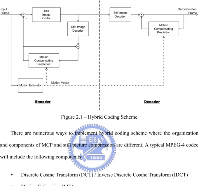
(15) represented in a more efficient and compact way to achieve high compression ratio. The redundancy exist between pixels in a frame is called “spatial redundancy”, and the similarity between temporally neighboring frames are “temporal redundancy”. To reduce the two kinds of redundancies can provide better video compression. Thus, to achieve the efficient video coding, the removal or reduction of the redundancies is addressed with video coding tools.. 2.1.1 Hybrid Coding Scheme The most commonly used video coding scheme is simple “hybrid coding scheme” as shown in Figure 2.1. The hybrid coding scheme can be considered as a derivation from differential pulse code modulation (DPCM). In addition, the hybrid coding scheme combines two kinds of techniques covering motion compensated prediction (MCP) and still picture compression for improving the coding efficiency. The MCP, which is described in section 2.2, is used to reduce the temporal redundancy. In addition, the still picture compression techniques can remove or reduce spatial redundancy. Existing technologies of MCP and still picture compression have been widely used in various areas. In addition, the hybrid coding scheme can be realized in software realization or hardware circuits. In addition, Figure 2.1 shows that the decoder in the scheme is simpler than the encoder and suitable for the case that a video sequence is encoded once and decoded many times. Because there are many advantages of hybrid coding scheme [2], the hybrid coding scheme comes to be the state-of-the-art architecture for video data exchange [3]. Thus, the hybrid coding scheme has been adopted in various modern video coding standards covering H.261, H.263, H.264, MPEG-1, MPEG-2, and MPEG-4.. -5-.

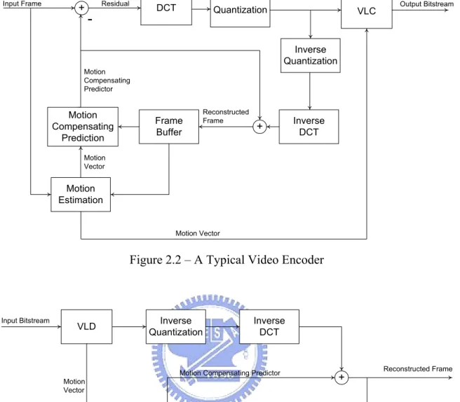
(16) Input Frame. +. Still Image Coder. -. Still Image Decoder. Reconstructed Frame. + Motion Compensating Prediction. Still Image Decoder. + Motion Compensating Prediction. Motion Estimator. Motion Vector. Encoder. Decoder. Figure 2.1 – Hybrid Coding Scheme There are numerous ways to implement hybrid coding scheme where the organization and components of MCP and still picture compression are different. A typical MPEG-4 codec will include the following components: Discrete Cosine Transform (DCT) / Inverse Discrete Cosine Transform (IDCT) Motion Estimation (ME) Motion Compensation (MC) Quantization / Inverse Quantization Variable-Length Coding (VLC) / Variable-Length Decoding (VLD) Frame Buffer The encoder and decoder consist of some of the components above are shown in Figure 2.2 and Figure 2.3 respectively.. -6-.

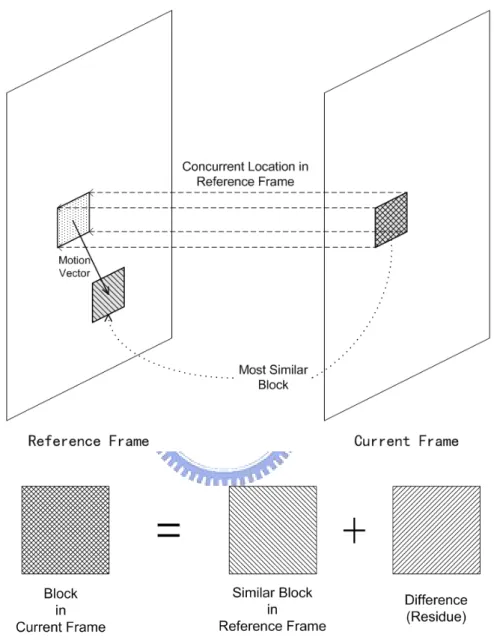
(17) Input Frame. +. Residual. DCT. -. Quantization. VLC. Output Bitstream. Inverse Quantization Motion Compensating Predictor. Motion Compensating Prediction. Frame Buffer. Reconstructed Frame. +. Inverse DCT. Motion Vector. Motion Estimation. Motion Vector. Figure 2.2 – A Typical Video Encoder. Input Bitstream. VLD. Inverse Quantization. Inverse DCT. Motion Compensating Predictor Motion Vector. Motion Compensating Prediction. +. Reconstructed Frame. Frame Buffer. Figure 2.3 – A Typical Video Decoder. 2.2. Motion Compensated Prediction Prediction is a common technique in data compression while correlations usually exist in. discrete signals. It is possible to predict current value from past or future signals, so do video sequence because the contents in frames are similar. A frame is divided into objects (or simply rectangular blocks), and similar objects in adjacent frames can be found and thought as the same object. The current object is described in motion vector (MV) and the difference (residue) between itself and its predictor as shown in Figure 2.4. The MV and residue can be -7-.

(18) coded and used with reference frame to predict the object in current frame. This is why it is named “motion compensated prediction” for that it utilizes the relationship of motion between frames to predict video signals.. Figure 2.4 – Motion Compensated Prediction The reference frame and motion vector are essential elements for MCP and two issues are derived from them: 1.. The accuracy of motions. 2.. The source of reference frame. -8-.

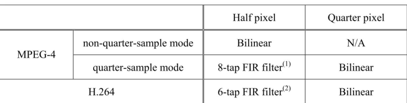
(19) For the first issue, because the video sequences are obtained by spatial and temporal sampling of video signals, the MVs are often represented as multiples of the horizontal and vertical sampling intervals (pixels or pels). Since the true frame-to-frame motions of the video contents are completely unrelated to the spatial sampling structure of video signal, we expect to improve MCP with the employment of MVs at subpixel accuracy, in which the MVs are represented as fractions rather than integers only [4], [5]. In practical implementation of video. 1 1 coding, the MVs are shown as ( x × ( ) n , y × ( ) n ) , where n ∈ N , x, y ∈ Z . 2 2. Pixels at fractional positions in the reference frame are needed with MCP at subpixel accuracy. However, they do not exist in reality and have to be generated via interpolation. There are kinds of interpolation filters used in image processing – bilinear, bi-cubic, finite impulse response low-pass filters (FIR-LPFs), Wiener filter, or other methods on frequency domain. As complexity is always one of the main considerations during video coding, modern video coding standards usually limit the accuracy of motion to quarter (1/4) pixels and the bilinear and separable FIR filters with few taps are often used during fractional pixel generation. For example, the interpolation filters adopted by MPEG-4 and H.264 are bilinear filter and FIR-LPFs, which are shown in Table 2.1.. Table 2.1 – Interpolation Filters in MPEG-4 and H.264. MPEG-4. Half pixel. Quarter pixel. non-quarter-sample mode. Bilinear. N/A. quarter-sample mode. 8-tap FIR filter(1). Bilinear. 6-tap FIR filter(2). Bilinear. H.264 [ Note ]. (1) Coefficients of 8-tap FIR filter: (-8, 24, -48 160, 160, -48, 24, -8) / 256 (2) Coefficients of 6-tap FIR filter: (1, -5, 20, 20, -5, 1) / 32. -9-.

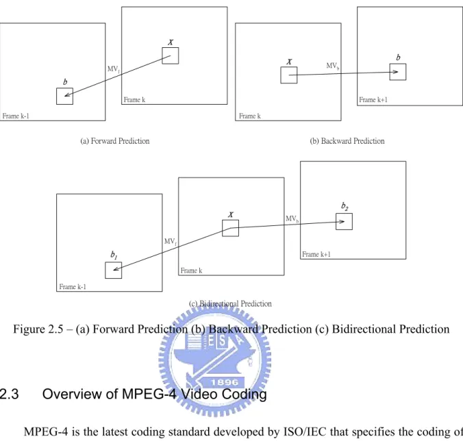
(20) The 2nd issue relates to the prediction schemes of video coding, which can be classified as three: 1. Forward prediction – Using past frame to predict current image contents. 2. Backward prediction – Using future frame to predict current image contents. 3. Bidirectional prediction – Using both past and future frames to predict current image contents. The relationship of MVs and reference frames in the three prediction schemes above are shown in Figure 2.5 while frame k is the current frame. In forward or backward prediction, the reference frame is the past or the future frame. Since the adjacent frames are likely to provide better motion compensation predictors, the most neighboring frames are usually chosen. In another case, the motion compensation predictor in bidirectional prediction is generated through a temporal interpolation process. As shown in Figure 2.5 (c), the motion compensation predictor xˆ of block x is given by xˆ = c1b1 + c2b2. 0 ≤ c1 , c2 ≤ 1. c1 + c2 = 1. b1 and b2 are the blocks in the past and the future frame with displacements of MVf and MVb correspondingly. The c1 and c2 are usually decided according to the temporal distance between the current and the two reference frames or simply set to 1/2, which means the predictor is the average of the two referenced blocks. The bidirectional prediction has the advantage that the motion compensated averaging over two frames may provide better predictor for video coding than prediction from one frame only. Thus, it is often used even if it is more complicated than the forward and backward prediction.. - 10 -.

(21) x x. MVf. b MVb. b Frame k. Frame k+1. Frame k-1. Frame k. (a) Forward Prediction. (b) Backward Prediction. x. b2 MVb. MVf. b1. Frame k+1 Frame k. Frame k-1. (c) Bidirectional Prediction. Figure 2.5 – (a) Forward Prediction (b) Backward Prediction (c) Bidirectional Prediction. 2.3. Overview of MPEG-4 Video Coding MPEG-4 is the latest coding standard developed by ISO/IEC that specifies the coding of. audio-visual objects. The part 2 of MPEG-4 relates to the video coding, if no special explanation is given, the word “MPEG-4” referred in the following text is the part 2 of MPEG-4 [1]. MPEG-4 supports the functionalities already provided by MPEG-1 [6] and MPEG-2 [7] and extend them to “content-based coding”, with which the video contents (e.g. the physical objects in a scene) are separated encoded and decoded [8]. To enable the content-based coding, MPEG-4 introduces the concepts of video objects (VOs) and video object planes (VOPs). A VO in a scene is an entity that a user is allowed to access and manipulate, and the instance of a VO at a given time is a VOP [1]. For the intra coding in MPEG-4, a VOP is. - 11 -.

(22) coded without any reference other than itself. For the inter coding in MPEG-4, a VOP is divided into rectangular blocks and the MCP coding is conducted on each block referencing other VOPs of the same VO. With this scheme, each VO can be coded/decoded independently. There are many functions in MPEG-4 including the coding of synthetic data, sprite, and still textures object, 3D mesh coding, scalable coding, ……etc. For the sake of simplicity, our discussions are focused on the coding of VOPs which are composed of rectangular blocks, and this kind of VOPs is the most commonly used in natural video data coding nowadays.. 2.3.1 Types of Video Object Plane According to the coding methods used, there are four types of VOPs [1]: 1.. Intra-coded VOP (I-VOP) – A VOP coded using information only from itself.. 2.. Predictive-coded VOP (P-VOP) – A VOP coded using MCP from a past reference VOP. 3.. Bidirectionally predictive-coded VOP (B-VOP) – A VOP coded using MCP from a past and/or future reference VOP(s).. 4.. Sprite VOP (S-VOP) – An S-VOP is a VOP for a sprite object or coded using prediction based on global motion compensation from a past reference VOP. It is in the range of sprite coding and will not be discussed in this thesis.. A VOP is regularly divided into 16x16 macroblocks (MBs), and each MB contains four 8x8 blocks. An MB in an I-VOP can be only INTRA coded where DCT, quantization, AC / DC prediction, and VLC are applied to the MB in order. An MB in a P-VOP can be either INTRA coded as if it is in an I-VOP or INTER coded where the forward prediction in section. - 12 -.

(23) 2.2 is applied on MB level. The residue of an INTER coded MB is transformed with DCT, quantized, and coded with VLC. In addition to INTRA coding, there are four modes for INTER coding in a B-VOP, where the MCP processes of them are different: 1.. Forward mode The forward prediction is used.. 2.. Backward mode The backward prediction is used.. 3.. Bi-directional mode The bidirectional prediction is used, and the coefficients c1 and c2 mentioned in section 2.2 are set to 1/2.. 4.. Direct mode The bidirectional prediction and same coefficients of c1 and c2 as in bi-directional mode are used, but only one delta vector MVd is coded in direct mode. The calculation of MVf and MVb used for bidirectional prediction in this mode involves linear scaling the MV of collocated block in temporally next I-, or P-VOP [1]: MV f =. TRB × MVn + MVd TRD. MV b=. (TRB − TRD) × MVn TRD. MV b= MV f − MVn. , if MVd is zero. , if MVd is nonzero. - 13 -.

(24) MVn is the motion vector of collocated block in temporally next I-, or P-VOP, TRB is the temporal difference of the B-VOP and its past reference VOP, TRD is the temporal difference of the two reference VOPs. An example is shown in Figure 2.6, where frame 1 is a B-VOP, frame 0 and 3 are the reference VOPs, TRD = 3, and TRB = 1. MVf MVb MVn. 0. 1. 2. 3. Figure 2.6 – An Example of Bidirectional Prediction in Direct Mode [1]. 2.3.2 Tools and Profiles Each tool specifies one function in MPEG-4 and a profile defines the subset of the syntax and semantics in MPEG-4 and thereby the decoder capability required to decode a particular bitstream [1], [9]. The tool specifies the functionality of MCP at quarter-pel accuracy is the Q-Pel MCP, and the B-VOP specifies the bidirectional MCP. Table 2.2 lists the tools as to code/decode the video objects of simple profile (SP) and advanced simple profile (ASP), and other profiles in MPEG-4 can be found in [1]. SP defines a small set of tools for video coding and ASP includes two more tools, the B-VOP and Quarter-Pel MCP. The SP and ASP are suitable for our research and are chosen to examine the effects of applying MCP at quarter-pel accuracy and bidirectional MCP.. - 14 -.

(25) Table 2.2 – Tools for MPEG-4 SP and ASP [1] Video Object Types Visual Tools. 2.4. Simple. Advanced Simple. I-VOP. X. X. P-VOP. X. X. DC Prediction. X. X. AC Prediction. X. X. 4-MV, Unrestricted MV. X. X. Slice Resynchronization. X. X. Data Partitioning. X. X. Reversible VLC. X. X. Short Header. X. X. B-VOP. X. Method 1 / Method 2 Quantization. X. Interlace. X. Global Motion Compensation. X. Quarter-pel Motion Compensation (QPEL MCP). X. Motion Estimation Motion Estimation (ME) is an important image processing technique that is developed. for years and wildly used in various fields including image sequence analysis, machine vision, image sequence restoration, robotics, or video coding. The aim of motion estimation is to. - 15 -.

(26) estimate the motion of an object in one frame to another frame. The size of the object whose motion is estimated ranges from the whole frame to a small pixel. In this thesis, we will focus on the motion estimation techniques in video coding applications. Common ME techniques can be divided into three groups covering frequency-domain techniques, gradient / pel-recursive techniques, and block-matching techniques The frequency-domain techniques are based on the relationship of transformation coefficients (e.g. phase or magnitude) of the objects in frames. The additional operations of transformations make them complex and not suitable for real-time video coding applications. The gradient / pel-recursive techniques are originally developed for image sequence analysis and posses some features as dense and smooth motion field or the option to deal with complex motion models. When they are compared with the block-matching algorithms, experiment results shows that the gradient / pel-recursive techniques require more overhead motion information or result in higher displaced frame difference (DFD) energy [10]. In other words, they cost more bandwidth for transmission. As a result, the block-matching techniques are more adequate for video coding applications and widely adopted in modern video coding algorithms.. 2.4.1 Block-based Motion Estimation The block-based techniques of MCP have the advantage of low overhead motion information for that the same motion vectors are assigned to all the pixels within a block. Block-based motion estimation (BBME) is the process of obtaining these motion vectors for the block. In the translation motion model, the MV represents the translational movement of a block between the current frame and the reference one as it is described in section 2.2. It is very intuitive for someone to “match” the current “block” with those blocks in the reference - 16 -.

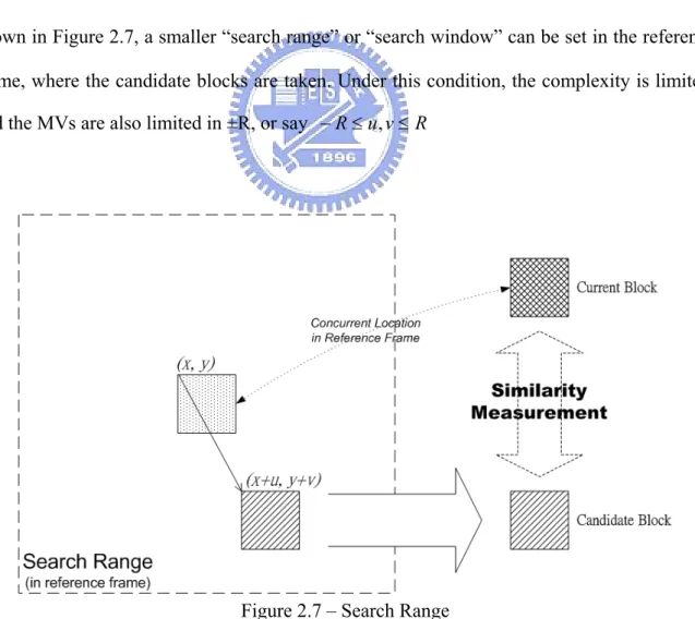
(27) frame in order to find the most similar one, and this is what was conducted in the block-matching ME. Blocks are taken with different locations in the reference frame as candidate blocks and evaluate the similarity / difference with the current block. The coordinate difference of the most similar candidate block and the current one will be coded as MV. Even though the most similar block may exist at any location in the reference frame, it is impractical to set the candidate locations of blocks to cover the whole frame due to the considerable computational complexity. In the natural video sequences, object motions between adjacent frames are usually limited and therefore the candidate blocks are located in a smaller area around the concurrent location of current block in the reference frame. As shown in Figure 2.7, a smaller “search range” or “search window” can be set in the reference frame, where the candidate blocks are taken. Under this condition, the complexity is limited, and the MVs are also limited in ±R, or say − R ≤ u, v ≤ R. Figure 2.7 – Search Range. - 17 -.

(28) 2.4.2 Criteria for Similarity The ME in video coding process provides MVs of motion compensation predictors, which will greatly affects the coding performance. Smaller differences between the to-be-coded block and its predictor bring better coding performance. Many criteria exist for the measurement of similarity between current and candidate blocks in ME, such as the cross-correlation or mean of squared error. Some common criteria are defined in the following list. MSE (Mean of Squared Error). [. ]. 1 2 Scurrent ( x, y ) − S reference ( x + u , y + v) ∑ wh x, y∈Block. MSE (u, v) =. SSE (Sum of Squared Error). ∑ [S. SSE (u , v) =. x, y∈Block. current. ( x, y ) − S reference ( x + u , y + v). ]. 2. MAD (Mean of Absolute Difference) MAD(u , v) =. 1 ∑ Scurrent ( x, y) − Sreference ( x + u, y + v) wh x , y∈Block. SAD (Sum of Absolute Difference) SAD(u , v) =. ∑S. x, y∈Block. current. ( x, y ) − S reference ( x + u , y + v). Scurrent(x, y) and Sreference(x, y) are the pixel value at coordinates (x, y) in the current and reference frame. (u, v) is the coordinate difference between current block and candidate block. The smaller SSE or SAD we get from two blocks, the higher similarity exists between them.. - 18 -.

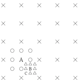
(29) Since the operations of floating-point number, square, or division may be needed with SSE, MSE, or MAD, the criterion of SAD is simpler and widely used in various video codecs.. 2.4.3 Sub-Pixel Motion Estimation There are various ways for ME at subpixel accuracy, as for block-based ME, the MVs are obtained with iteratively matching the current block with candidate blocks at fractional positions in the reference frame. There are two parts involved in BBME at subpixel accuracy: 1st—The composition of candidate blocks, and 2nd—The search methods. The candidate blocks are groups of pixels at fractional positions generated via interpolation process described in section 2.2. Figure 2.8 is a simple example shows 3x3 candidate blocks at different positions, where the capitalized letters are integer pels (pixels at integer positions) and the others are half pels (pixels at half-pixel positions). The candidate ⎡A B block ⎢⎢ D E ⎢⎣G H ⎡ a 2 b2 ⎢d 2 e2 ⎢ ⎢⎣ g 2 h 2. C⎤ ⎡ a1 b1 c1 ⎤ ⎥ F ⎥ is in position (0, 0), and the others are ⎢⎢ d1 e1 f 1⎥⎥ in (0.5, 0), ⎢⎣ g1 h1 i1 ⎥⎦ I ⎥⎦. c2 ⎤ ⎡ a 3 b3 ⎥ f 2⎥ in (0, 0.5), and ⎢⎢ d 3 e3 ⎢⎣ g 3 h3 i 2 ⎥⎦. c3 ⎤ f 3⎥⎥ in (0.5, 0.5). While it is in other cases, i3 ⎥⎦. candidate blocks with larger size and at quarter-pixel positions can be derived in a similar way.. - 19 -.

(30) A. a1. B. B1. C. c1. a2. a3. b2. B3. c2. c3. D. d1. E. E1. F. f1. d2. d3. e2. E3. f2. f3. G. g1. H. H1. I. i1. g2. g3. h2. H3. i2. i3. Figure 2.8 – An Example of Candidate Blocks at Fractional Position The method to find the best matching candidate block is full search (FS), where all the candidate blocks in search range will be searched to find the one with the smallest differences. It is very inefficient, and, since modern video coding standards usually include MCP at quarter-pixel accuracy, there will be 16 times of candidate blocks compared to those in ME at integer-pixel accuracy. A compromise arises that FS is conducted at integer-pixel level to find the best integer-pixel position, and then, based on the result of integer-pixel level, search the 8 surrounding half-pixel positions to find the best half-pixel position. After all, the final position is got with searching the 8 quarter-pixel positions surrounding the result of half-pixel level. It is shown in Figure 2.9, where the symbols ╳, ○, △ are candidate positions at integer-, half-, and quarter-pixel levels, and A, B, C denote the search results at integer-, half-, and quarter-pixel levels correspondingly. The FS with levels is widely used as benchmark for the development of ME at subpixel accuracy.. - 20 -.

(31) A B C. Figure 2.9 – Full Search with Three Levels. 2.4.4 Motion Estimation for B-VOPs in MPEG-4 Motion estimation for B-VOPs in MPEG-4 involves the estimation of MVs for the four modes mentioned in Section 2.3.1, which becomes more complicated than ME for forward prediction only. The methods for the four modes are described as follows. 1.. Forward mode – The candidate blocks are taken from past reference frame and examined to find the best predictor.. 2.. Backward mode –The candidate blocks are taken from future reference frame and examined to find the best predictor.. 3.. Bidirectional mode – The candidate blocks are generated as described in section 2.2 and 2.3.1 with MVf and MVb. If every combination of possible positions of forward and backward motion is examined, the complexity will be large. For example, let the search range for forward and backward motion in bidirectional mode to be both. ± R , the number of all possible combination is 16R4, which is much larger than the numbers (4R2) in forward or backward mode. An alternative way is to use the MVs found in forward and backward mode as the MVs in bidirectional mode. Although - 21 -.

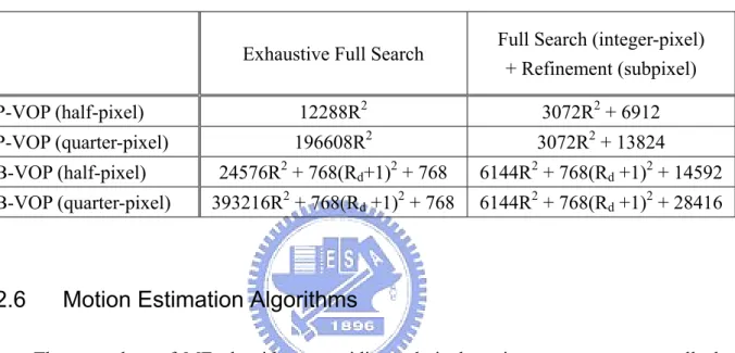
(32) this combination may not result the best predictor, the complexity would be more acceptable, and this method is implemented in the MPEG-4 VM. 4.. Direct mode – Since the MV of co-located block in the next reference frame has been determined before the ME for direct mode, the candidates of forward and backward motion can be limited according the range of delta vector MVd, which is often much smaller than the search ranges in forward and backward modes. The candidate blocks are generated as described in section 2.3.1 with different delta vectors and examined to find the best predictor.. 2.5. Computational Complexity The computational complexity of searching the MV of a block consists of three parts –. search points, matching pixels, and operations of evaluating difference. The search points are the positions of candidate blocks. The matching pixels are the pixels participating in evaluating block difference. In common cases, the number of matching pixels of a 16x16 MB is 16 × 16 = 256 . The operations of evaluating difference of a pixel are 1subtraction + 1absoluting + 1addition = 3, when SAD is used. Let the search window to be 2 R × 2 R in integer pixel, when 3-level full search is used, the total operations of ME of an MB to quarter-pixel accuracy are (4 R 2 + 9 + 9) × 256 × 3 = 3072 R 2 + 13824 .. If the same 3-level full search is used in forward and backward mode of B-VOP, the MVf and MVb in forward and backward mode are used in bidirectional mode, and the search radius in direct mode is Rd, the operations of ME at quarter-pixel accuracy for an MB in B-VOPs are summarized. For each MB, the forward mode needs 3072R2 + 13824 operations, the backward mode requires 3072R2 + 13824 operations, the bidirectional mode has 256 × 3 = 768 operations, and the direct mode takes ( Rd + 1) 2 × 256 × 3 = 768( Rd + 1) 2. - 22 -.

(33) operations. Thus, 3-level full search will take 6144R2 + 768(Rd +1)2 + 28416 operations per MB in total. The operations of pixel averaging in bidirectional and direct mode are not included above. The complexity of ME for an MB in a P-VOP or a B-VOP with different motion accuracy is shown in Table 2.3.. Table 2.3 – Computational Complexity of Motion Estimation for a Macro Block Exhaustive Full Search. Full Search (integer-pixel) + Refinement (subpixel). P-VOP (half-pixel). 12288R2. 3072R2 + 6912. P-VOP (quarter-pixel). 196608R2. 3072R2 + 13824. 24576R2 + 768(Rd+1)2 + 768. 6144R2 + 768(Rd +1)2 + 14592. 393216R2 + 768(Rd +1)2 + 768. 6144R2 + 768(Rd +1)2 + 28416. B-VOP (half-pixel) B-VOP (quarter-pixel). 2.6. Motion Estimation Algorithms The procedure of ME algorithms providing subpixel motion accuracy can usually be. divided in to two portion covering finding the MV at integer-pixel accuracy and then refining the MV at subpixel accuracy. The methods dealing with the MV refinement at subpixel accuracy can be categorized as two groups consisting of block matching with levels and difference approximation methods. The former is conventional, while it is intuitive that refinement are conducted level by level and the subpixel positions around the one pointed with MV from upper level are searched. It has the advantage of regularity and the disadvantages of possibly higher complexity, higher memory bandwidth, and the need of interpolation of pixels. The latter approximates the block differences at subpixel positions with a given model instead of block matching. It avoids the operations from matching of blocks and interpolation of pixels but. - 23 -.

(34) introduces some constrains and extra computations in addition. Some modern subpixel ME algorithms belong to the latter are discussed in the following section.. 2.6.1 Sub-Pixel Motion Estimation with Block Difference Approximation Methods The subpixel ME algorithms of block difference approximation all have their own models, which are linear, quadratic, parabolic, …and so on. The core of a block difference approximation method is to solve the parameters of the model. Block differences at subpixel positions are got through calculation without the real matching of blocks. In [11], a quadratic-like model is assumed in IMAM as to estimate the mean absolute error/difference (MAE / MAD) at half-pixel positions. The positions with the minimal estimated MAE is chosen as the MV of half-pixel accuracy. A hybrid method named PPHPS of combining the difference approximation and block matching is proposed in [12]. A parabolic function is used as to model the SAD at half-pixel positions. With the SADs of surrounding integer positions, unknown parameters of the function are calculated. Instead estimating all values at half-pixel positions, a predicted position is found at the minimum of the function, and block matching of three search points is executed to get the true SADs and MV of half-pixel accuracy. Although fewer or no block matching processes exist in the block difference approximation methods, they all have the similar problems: 1.. The prediction accuracy depends on the models used. The adoption of a more complex model (from linear to quadratic or parabolic) may bring improvements on prediction accuracy, but also higher computational complexity. Meanwhile, the true error surface of SAD may not coincide with the model, and that is why block - 24 -.

(35) matching is still needed in PPHPS after the estimation of the half-pixel MV. The block matching is back again. 2.. Some constrains or limits are also introduced as the model of block difference is used. The SADs or MAEs surrounding the subpixel positions have to exist before computing the parameters of the model. When SADs of some positions in search range or around the border of search window may be missing with modern fast ME algorithms, the block difference approximation will not be applicable. In addition, due to the similar constrains of existent SADs, this kind of methods can only be carried out either in half-pixel level of in the quarter-pixel one. The interpolation and matching processes are still needed in the other level.. From the discussions above, the matching between blocks seems to be inevitable with an ME algorithm providing quarter-pixel motion accuracy. In the method we proposed, block-matching is still used, which is more regular for hardware implementation, and interpolation process during the matching in subpixel level is avoided.. 2.6.2 Binary Hierarchical Motion Estimation Multiresolution techniques have been proposed as to reduce the computational complexity of ME [18], [19]. A hierarchical search will be performed from lower to higher resolution levels and the MV is refined level by level. Furthermore, binary ME algorithms are developed to reduce the computational complexity and memory bandwidth by reducing the pixel depth to one bit [13]-[16]. All these methods focus on motion search above integer level and still need 8-bit block matching at subpixel levels rather than the binary representation. Based on the concept of binary hierarchical motion search, we develop the ME providing subpixel motion accuracy, which is also applicable in B-VOPs of MPEG-4.. - 25 -.

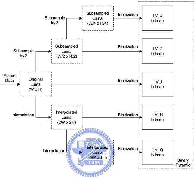
(36) Chapter 3 Fractional Pixel Binary Motion Estimation. The fractional pixel binary motion estimation (FPBME) supporting subpixel motion accuracy and motion search in B-VOPs is presented in this chapter. This method is based on binary hierarchical motion estimation and makes use of the spatial-temporal correlations in motion vector field to achieve low complexity and good visual quality. A simple strategy to improve rate-distortion performance in MPEG-4 ASP is also introduced in later section of this chapter.. 3.1. Binary Pyramidal Structure The binary pyramidal structure is the core of our method. The luminance of each frame. in video sequence is processed with filters to generate layers of binary data with different spatial resolutions. As shown in Figure 3.1, the luminance data are subsampled with subsampling filters and then binarized into bitmap. Pixels at fractional positions are interpolated and binarized into bitmap with larger size. Every pixel in the bitmap is of one-bit width, which stores the binary feature. The bitmaps including Lv_4, Lv_2, Lv_I, Lv_H, and Lv_Q (if QPEL MCP is used) constitute the binary pyramid of a certain frame (or VOP).. - 26 -.

(37) Subsample by 2. Subsampled Luma (W/2 x H/2). Subsample by 2. Frame Data. Subsampled Luma (W/4 x H/4). Original Luma (W x H). Interpolation. Interpolated Luma (2W x 2H). Interpolation. Interpolated Luma (4W x 4H). Binirization. LV_4 bitmap. Binirization. LV_2 bitmap. Binirization. LV_I bitmap. Binirization. LV_H bitmap. Binirization. LV_Q bitmap Binary Pyramid. Figure 3.1 – Construction of Binary Pyramid. 3.2. Subsampling and Interpolation The luminance data are subsampled to achieve image with lower resolution. Low pass. filters may be needed to avoid aliasing. There are three ways for subsampling. Direct Subsampling. - 27 -.

(38) No anti-aliasing filter is used. Pixels at even coordinates are directly used without any processing. The advantage of this is very low complexity where no extra operations are needed, but aliasing may happen. Mean filter As shown in Figure 3.2, mean of four pixels (A, B, C, D) are used as the subsampled pixel value. …. …C. B. …. …. …A. …. D. …. …. … …. …. …. Figure 3.2 – Mean Filter during Subsampling. 3-tap Low-Pass Filter A serapable 3-tap low-pass filter is used as the anti-aliasing filter during subsampling. The filter coefficients are. [1. 2 1] ÷ 4. The use of 3-tap LPF will slightly increase the complexity of subsampling but avoid aliasing. The filters used in interpolation process depend on usage of QPEL MCP. In MPEG-4, as shown in Table 2.1, if sequence is coded without QPEL MCP, bilinear filter is used to generate the half pixels, and interpolation for quarter pixels is not conducted. When QPEL MCP is adopted, the half pixels are generated with 8-tap FIR filter of. - 28 -.

(39) [− 8. 24 − 48 160 160 − 48 24 − 8] ÷ 256. , and the quarter pixels are then calculated with bilinear filtering the integer and half pixels.. 3.3. Binarization The depths of pixels are reduced to one bit width through binarization. Since human eyes. are more sensitive to edges and high frequency regions, which are distinct from their neighbors, this regions or pixels are more important for human vision. This kind of feature pixels can be extracted through the comparison between pixel value (x) and threshold (TH) from low-pass filtering the local region, which is ⎧1 , x > TH y=⎨ ⎩0 , otherwise. For this reason, low-pass filters are used to produce the bitmaps with binary features. Various filters are discribed in the following sections.. 3.3.1 Filters in Integer and Subsampled Levels The same filtering process is conducted in Lv_I, Lv_2, and Lv_4 except the different dimensions of levels. The filter is first applied on luminance data of frame in Lv_I, or pixels after downsampling in Lv_H and Lv_Q as to get a threshold for a pixel. After the filtering, the pixel value is compared with its threshold to decide the binary value, 0 or 1, of it. This process is executed repeatedly to generate all the binary data of each level. The filters mentioned above can maybe changed and described in the following.. - 29 -.

(40) Mean of 4 surrounding pixels (M4) As shown in Figure 3.3, the threshold of pixel X (center pixel) is. TH X =. A+ B +C + D +1 4 C B. X. A. D. Figure 3.3 – Threshold from Mean of 4 Surronding Pixels. Mean of 8 surrounding pixels (M8) As shown in Figure 3.4, the threshold of pixel X is. TH X =. A+ B +C + D + E + F +G + H +1 8 A. B. C. D. X. E. F. G. H. Figure 3.4 – Threshold from Mean of 8 Surronding Pixels. N-tap FIR filters FIR filters with increasing tap numbers have better frequency response, but cause more complexity to binarization process. A separable 13-tap Hamming filter with 30% of cut-off frequency is introduced for better binarization:. [− 82,−295,−475,580,3819,7918,9830,7918,3819,580,−475,−295 − 82] ÷ 32760 - 30 -.

(41) 3.3.2 Filters in Sub-Pixel Levels Because the candidate blocks at subpixel positions are got from a subsample-like process as shown in section 2.4.3, the filters mentioned in last section cannot be directly applied to the interpolated frame data. The threshold of a pixel of integer-pixel position in subpixel levels should be generated from filtering neighboring integer pixels instead of half or quarter pixels. For example, if the filter M4 is used for binarization, the threshold for the pixel E in Figure 2.8 should be decided from averaging the integer pixels of B, D, F, and H, instead of half pixels of b2, d1, e1, and e2. The same concept is suitable for half and quarter pixels. The solution to this problem is to modify binarization filters as follows. Mean of 4 surrounding pixels at subpixel levels The referenced pixels by the filter can be expressed as (x+2, y), (x-2, y), (x, y-2), (x, y+2) in Lv_H (x+4, y), (x-4, y), (x, y-4), (x, y+4) in Lv_Q where (x, y) is the pixel to decide the threshold for.. Mean of 8 surrounding pixels at subpixel levels The referenced pixels by the filter can be expressed as (x+2, y+2), (x+2, y+2), (x-2, y+2), (x, y-2), (x, y+2), (x-2, y+2), (x-2, y), (x-2, y-2) in Lv_H. - 31 -.

(42) (x+4, y+4), (x+4, y+4), (x-4, y+4), (x, y-4), (x, y+4), (x-4, y+4), (x-4, y), (x-4, y-4) in Lv_Q where (x, y) is the pixel to decide the threshold for.. N-tap FIR filters at subpixel levels The 13-tap filter is modified as [-82, 0, -295, 0, -475, 0,580, 0, 3819, 0, 7918, 0, 9830, 0, 7918, 0, 3819, 0, 580, 0, -475, 0, -295, 0, -82] ÷ 32760 in Lv_H [-82, 0, 0, 0, -295, 0, 0, 0, -475, 0, 0, 0, 580, 0, 0, 0, 3819, 0, 0, 0, 7918, 0, 0, 0, 9830, 0, 0, 0, 7918, 0, 0, 0, 3819, 0, 0, 0, 580, 0, 0, 0, -475, 0, 0, 0, -295, 0, 0, 0, -82] ÷ 32760 in Lv_Q Although the modified filters described above seem to be much more complicated than those in section 3.3.1, regularities can be found that the distances between referenced pixels and center pixel in Lv_H and Lv_Q are twice and 4 times as those in Lv_I correspondingly. They can be easily handled during the implementation of software or hardware with regularly access these referenced pixels. The filters at subpixel levels cause only little more complexity and are still applicable.. - 32 -.

(43) 3.4. Matching Criterion Compared to the criteria in section 2.4.2, simpler criterion for measuring similarity can. be used when one pixel is represented in a single bit. The criterion used during binary block matching is SOD (sum of differences) and is defined as SOD(u, v) =. ∑ [S. x, y∈Block. current. ( x, y ) ⊕ S reference ( x + u, y + v). ]. Scurrent(x, y) and Sreference(x, y) are the binary representations at coordinates (x, y) in the current and reference frame. (u, v) is the coordinate difference between current block and candidate block. The symbol ⊕ denotes the one-bit XOR operation. The characteristics of SOD are 1.. SOD has less computational complexity than SAD, since no extra operation needed to handle the sign information.. 2.. XOR is easy to be implemented in hardware.. 3.. Even without dedicated hardware, pixels with binary representation can be put together in a single register of processor and compared simultaneously.. Similar to SAD, higher SOD means more differences and less similarities exist between two binary blocks.. 3.5. Search Flow The proposed search flow is simple and straightforward. As shown in Figure 3.5, the. motion search for a block starts from Lv_4, goes top-down through levels, and ends after the refinement search with candidates. The only decision made between levels is the usage of - 33 -.

(44) QPEL MCP. If QPEL MCP is not enabled, Lv_Q search is skipped, and the refinement search with candidates will be conducted right after the Lv_H. Details of searching in each level are described in the following sections. For the simplicity of descriptions, the block size of 16 and search range of (-R ~ +R) in integer pixels are assumed without loss of generality.. LV_4 Full Search mv_4. LV_2 Search mv_2. LV_I Search mv_I. LV_H Search mv_H. QPEL MCP ?. Y. LV_Q Search. N. mv_Q. Refinement Search with Candidates Final motion vector. Figure 3.5 – Search Flow. 3.5.1 Lv_4 Search Full search with search range (−. R R ~ + ) is conducted in this level. The 4x4 blocks 4 4. from the Lv_4 bitmap in the binary pyramid of current and reference frame are matched iteratively as to find the motion vector, mv_4, which results the minimal SOD.. - 34 -.

(45) 3.5.2 Top-Down Hierarchical Search From Lv_2 to Lv_Q, motion vector from the upper level will be scaled by 2, and a search of search range ± 1 will be conducted around the position pointed by the scaled motion vector. The position with the minimal SOD will be taken as the motion vector of this level and passed to lower level. Details of each level are shown in Table 3.1.. Table 3.1 – Details of Lv_2 to Lv_Q Lv_2. Lv_I. Lv_H. Lv_Q. Block Size. 8x8. 16x16. 16x16. 16x16. Source of Block. Lv_2 bitmap. Lv_I bitmap. Lv_H bitmap. Lv_Q bitmap. Search Range. (-1 ~ +1). (-1 ~ +1). (-1 ~ +1). (-1 ~ +1). Search Points. 9. 9. 9. 9. 3.5.3 Refinement with Candidates The spatial-temporal correlations in motion vector field will be utilized during this step. Motion vectors of the neighboring blocks (as shown in Figure 3.6) of the current block will be chosen as center of refinement search. The motion vectors are listed below: mv_UR: motion vector of upper right block mv_U: motion vector of upper block mv_L: motion vector of left block mv_CL: scaled motion vector of co-located block in reference frame mv_Z: zero motion. - 35 -.

(46) Because motion estimation will also be executed to get the forward and backward motion vectors in B-VOP, the mv_CL will be adjusted according to the reference frame as: Forward motion estimation in P-VOP mv _ CL = MV past. Forward motion estimation in B-VOP. mv _ CL =. TRB MV past TRD. Backward motion estimation in B-VOP. mv _ CL =. TRB − TRD MV future TRD. MVpast and MVfuture are the motion vector of co-located blocks in past and future reference frame correspondingly. TRB is the temporal difference of current B-VOP and previous P-VOP. TRD is the temporal difference of previous and next P-VOPs, where B-VOPs are in between. Blocks in this step come from the Lv_Q when QPEL MCP is enabled. If QPEL MCP is disabled, blocks in Lv_H will be used instead. Refinement search of search range ± 1 will be conducted around the position pointed by these five motion vectors as to improve the accuracy of motion estimation. The MV with minimal SOD in this step will be compared with the result from last step, and the MV with smaller SOD will be the final MV of the block.. - 36 -.

(47) Block_U. Block_L. Block_UR. Current Block. Block_CL. Figure 3.6 – Candidates in Candidate Refinement Search Step. 3.6. Complexity Analysis Let the search range in integer pixel to be R ( − R ~ + R ), the computational complexity. of the proposed subpixel binary motion estimation is shown in Table 3.2. While comparing the proposed method with FS, the complexity reduction is large. Table 3.2 – Computational Complexity of Each Level LV_4 LV_2 LV_I LV_H Full Search Half-pixel Accuracy. Total. Search Points. 4R2. 9. 4R2 + 9. Marching Pixels per Point. 256. 256. 1024R2 + 2304. Search Points. 4R2. 9. 9. 4R2 + 18. 256. 256. 256. 1024R2 + 4608. Full Search Quarter-pixel Marching Accuracy Pixels per Point FPBME Half-pixel Accuracy. LV_Q. Search Points. R2/4. 9. 9. 54. (R2)/4 + 72. Marching Pixels per Point. 16. 64. 256. 256. R2 + 18432. Search Points. R2/4. 9. 9. 9. 54. (R2)/4 + 81. 16. 64. 256. 256. 256. R2 + 19008. FPBME Quarter-pixel Marching Accuracy Pixels per Point. - 37 -.

(48) 3.7. Rate-Distortion Performance of MPEG-4 Advanced Simple Profile As shown in section 2.3.2, QPEL MCP and B-VOP are defined in MPEG-4 ASP. In this. section, we focus on the performance gains when applying B-VOP and QPEL MCP, and compare them with Simple Profile (SP). QPEL-MCP The performance gain of QPEL MCP is obvious since it provides better predictors and therefore reduces the texture bits when coding a video sequence.. B-VOP More reference VOP and various prediction modes of B-VOP help to improve the rate-distortion performance. However, when applying B-VOP in low-bitrate applications (especially in lower time resolution, such as 15 fps, 10fps…etc.), the performance might be worse than that of SP. For example, in the case of 2 B-VOPs between I- and P-VOPs (as in Table 3.3), the temporal distances between P-VOPs of ASP and their reference VOPs are 3, where those in SP are 1. The longer temporal distance and lower frame correlation often make VOP 3 and 6 in ASP cost more bits or have worse quality than those in SP, if the same quantization parameter (QP) is used in P- and B-VOPs.. Table 3.3 – An Example of Sequences Coded with or without B-VOPs Time index. 0. 1. 2. 3. 4. 5. 6. …. SP. I. P. P. P. P. P. P. …. ASP. I. B. B. P. B. B. P. …. - 38 -.

(49) The simplest solution is to set larger QP to B-VOPs and smaller QP to P-VOPs. it is, QPB−VOP = n × QPP−VOP , n > 1 Performances are improved with larger n as shown in Figure Figure 3.7. This results more distortions and lower bitrate in B-VOP, while less distortions and higher bitrate in P-VOP. The benefit is that, since P-VOPs are used as references of B-VOPs and successive P-VOPs, P-VOPs with less distortion retain more image information as to be better references during coding, and therefore the coding performance is improved. Simple comparisons between SP and ASP with different visual tools are shown in Figure 3.8. The video sequence is BUS, CIF (352x288), 15fps, and 3-level full search is used. When apply B-VOP, n = 1.5, and 2 B-VOPs are used between consecutive P-VOPs. SP + 2B. PSNR_Y. I=P=B. I=P, B=1.25P. I=P, B=2B. 34 33 32 31 30 29 28 27 26 25. bps 0. 100. 200. 300. 400. 500. 600. 700. 800. 900. Figure 3.7 – Rate-Distortion Performance with Different QP in B-VOPs. - 39 -. 1000.

(50) SP. PSNR_Y. SP + QPEL. SP + 2B. SP + 2B + QPEL. 34 33 32 31 30 29 28 27 26. bps. 25 0. 100. 200. 300. 400. 500. 600. 700. 800. 900. Figure 3.8 – Rate Distortion Performance with Different Visual Tools. 3.8. Merging of Bitmaps For the multi-resolution ME methods and for supporting fractional-pel ME, extra storage. is the common drawback, which is addressed based on the binary representation of pixels. With binary representation of pixel data, the extra storage size is smaller than the pyramidal structures for ME with more pixel depth. In addition, the bitmaps of Lv_I, Lv_H, and Lv_Q can be merged to reduce the memory required for binary pyramid. During the interpolation process, duplicate pixels at integer or half-pixel positions are kept in sub-pixel levels as shown in Figure 3.9. The binary values of the duplicate pixels at the same coordinate are identical when using similar binarization filters in Lv_I, Lv_H, and Lv_Q. The property of identical binary pixels makes it possible to merge the bitmaps of integer and sub-pixel levels. When FPBME is conducted at half-pixel accuracy, the bitmap of Lv_I is merged into the bitmap of Lv_H. When FPBME is conducted at quarter-pixel. - 40 -.

(51) accuracy, the bitmaps of Lv_I and Lv_H are both merged into the bitmap of Lv_Q. The bits required for a binary pyramid with or without bitmap merging is shown in Table 3.4, in which W and H are the width and height of a frame correspondingly. Since the bitmaps are merged, the computational complexity of pre-processing and the memory requirement of binary pyramid will both be reduced with the technique of bitmap merging.. Lv_I Lv_H Lv_Q. -1. -1.5. -0.5. 0. 0.5. 1. 1.5. Figure 3.9 – Duplicate Pixels in Lv_I, Lv_H and Lv_Q. Table 3.4 – Memory Reduction Achieved with Bitmap Merging Total Bits FBME Half-pixel Accuracy. No Bitmap Merging. 85 WH 16. Bitmap Merging. 69 WH 16. FBME Quarter-pixel Accuracy. No Bitmap Merging. 341 WH 16. Bitmap Merging. 261 WH 16. - 41 -. Reduction Rate. 18.82%. 23.46%.

(52) Chapter 4 Experimental Results. In this chapter, the experimental results of the fast fractional-pel motion estimation are provided.. 4.1. Simulations The test setup of our experiments: Test Operation System: Microsoft Windows XP professional Test Software: MPEG-4 Verification Model – MoMuSys FPDAM1-1.0-001220 Compiler: Microsoft Visual C++ 6.0 Common Test Configurations: No shape coding Deblocking Filter is disabled No rate control – the QPs are kept constant during coding a sequence. H.263 quantization mode is selected. Rounding Control is enabled. Initial value for Rounding Control : 0 Error Resilience mode is disabled. NEWPRED is not used. AC/DC prediction of Intra macroblocks is enabled. COMBINED motion/shape/texture coding will be used No SPRITE Usage - 42 -.

(53) Search range per coded frame: 16 Test sequences: Akiyo, Foreman, Mobile-and-Calendar, (Coastguard, Container, Stefan) in CIF (352x288), YUV 4:2:0 Other configurations will be described in the following sections.. 4.2. Performance Comparisons The rate-distortion performance of different conditions is shown in figure. The. distortions are represented with PSNR (peak signal-to-noise rate). The rate control is disabled for that the rate-distortion performance of motion estimation will be shown without influences of the scheme of rate control. The figures are plotted with data of PSNR and bitrates gathered via coding the test sequence with different quantization parameters listed in the following. No B-VOP usage (IPP) QPI = QPP = 4, 8, 16, 24, 31 Two B-VOPs between I- or P-VOPs (IBBP) QPI = QPP = 4, 8, 16, 24 QPI = 1.25 QPP = 5, 10, 20, 30 The results of the proposed method will be compared with those of FS.. - 43 -.

(54) 4.2.1 Impact of Refinement Search with Candidates on Coding Efficiency The effects of the step of refinement search with candidates are shown in Figure 4.1 to Figure 4.3. The sequence is coded at the frame rate of 30 fps. Motion estimation with or without the step of refinement search with candidates are denoted as “CRS (candidate refinement search)” and “No CRS.” As can be seen in this figures, the improvement of 1 ~ 4dB in PSNR_Y can be achieved with CRS.. Akiyo, H-pel, IPP 42. 40. PSNR-Y. 38. CRS No CRS. 36. 34. 32. 30 0. 50000. 100000. 150000. 200000 bps. (a). - 44 -. 250000. 300000. 350000.

(55) Akiyo, Q-pel, IPP 42. 40. PSNR-Y. 38. CRS No CRS. 36. 34. 32. 30 0. 50000. 100000. 150000. 200000. 250000. 300000. 350000. bps. (b) Akiyo, H-pel, IBBP 42. 40. PSNR-Y. 38 CRS No CRS. 36. 34. 32. 30 0. 50000. 100000. 150000. 200000. bps. (c). - 45 -. 250000. 300000.

(56) Akiyo, Q-pel, IBBP 42. 40. PSNR-Y. 38 CRS No CRS. 36. 34. 32. 30 0. 50000. 100000. 150000. 200000. 250000. 300000. bps. (d) Figure 4.1 – R-D of Akiyo with and without CRS: (a) Half-pixel, IPP (b) Quarter-pixel, IPP (c) Half-pixel, IBBP (d) Quarter-pixel, IBBP Foreman, H-pel, IPP 39. 37. PSNR_Y. 35 CRS No CRS. 33. 31. 29. 27 0. 500000. 1000000. 1500000 bps. (a). - 46 -. 2000000. 2500000.

(57) Foreman, Q-pel, IPP 39. 37. CRS No CRS. 33. 31. 29. 27 0. 200000. 400000. 600000. 800000. 1000000 1200000 1400000 1600000 1800000 2000000 bps. (b) Foreman, H-pel, IBBP 39. 37. 35 PSNR_Y. PSNR_Y. 35. CRS No CRS. 33. 31. 29. 27 0. 200000 400000 600000 800000 1000000 1200000 1400000 1600000 1800000 2000000 bps. (c). - 47 -.

(58) Foreman, Q-pel, IBBP 39. 37. PSNR_Y. 35. CRS No CRS. 33. 31. 29. 27 0. 200000. 400000. 600000. 800000. 1000000. 1200000. 1400000. 1600000. 1800000. bps. (d) Figure 4.2 – R-D of Foreman with and without CRS (a) Half-pixel, IPP (b) Quarter-pixel, IPP (c) Half-pixel, IBBP (d) Quarter-pixel, IBBP Mobile, H-pel, IPP. 36 34. PSNR-Y. 32 30. CRS No CRS. 28 26 24 22 0. 1000000. 2000000. 3000000. 4000000. bps. (a). - 48 -. 5000000. 6000000.

(59) Mobile, Q-pel, IPP. 36 34. PSNR-Y. 32 30. CRS No CRS. 28 26 24 22 0. 500000 1000000 1500000 2000000 2500000 3000000 3500000 4000000 4500000 5000000 bps. (b) Mobile, H-pel, IBBP. 36. 34. PSNR-Y. 32. 30. CRS No CRS. 28 26. 24. 22 0. 1000000. 2000000. 3000000. 4000000. bps. (c). - 49 -. 5000000. 6000000.

(60) Mobile, Q-pel, IBBP. 36. 34. PSNR-Y. 32. 30. CRS No CRS. 28. 26. 24. 22 0. 500000. 1000000 1500000 2000000 2500000 3000000 3500000 4000000 4500000 bps. (d) Figure 4.3 – R-D of Mobile with and without CRS (a) Half-pixel, IPP (b) Quarter-pixel, IPP (c) Half-pixel, IBBP (d) Quarter-pixel, IBBP. 4.2.2 Impact of Binarization Filters on Coding Efficiency The R-D curves of sequences coded with different binarization filters described in section 3.3 are shown in Figure 4.4 to Figure 4.6. The notation of subsampling and binarization filters is shown in Table 4.1. Table 4.1 – Notations of Subsampling and Binarization Filters Filters Subsamplig. Binarization. S0 – Direct Subsampling. B1 – Mean of 4 surrounding pixels. S1 – Mean Filter. B2 – Hamming, 13-tap, 30% Cut-Off Frequency. S2 – 3-tap Low-Pass Filter. B3 – Mean of 8 surrounding pixels. - 50 -.

(61) Akiyo, H-pel, IPP 42 41 40 39. PSNR-Y. 38 Full Search. 37. S2 B1. 36. S2 B2. 35. S2 B3. 34 33 32 31 30 0. 50000. 100000. 150000. 200000. 250000. 300000. bps. (a) Akiyo, Q-pel, IPP 42 41 40 39. PSNR-Y. 38. Full Search. 37. S2 B1. 36. S2 B2. 35. S2 B3. 34 33 32 31 30 0. 50000. 100000. 150000. 200000. bps. (b). - 51 -. 250000. 300000.

(62) PSNR-Y. Akiyo, H-pel, IBBP 42 41 40 39 38 37 36 35 34 33 32 31. Full Search S2 B1 S2 B2 S2 B3. 0. 50000. 100000. 150000. 200000. 250000. bps. (c) Akiyo, Q-pel, IBBP 42 41 40. PSNR-Y. 39 38. Full Search. 37. S2 B1. 36. S2 B2. 35. S2 B3. 34 33 32 31 0. 50000. 100000. 150000. 200000. 250000. bps. (d) Figure 4.4 – R-D of Akiyo Sequence: (a) Half-pixel, IPP (b) Quarter-pixel, IPP (c) Half-pixel, IBBP (d) Quarter-pixel, IBBP. - 52 -.

(63) Foreman, H-pel, IPP 39 38 37 36. PSNR-Y. 35 Full Search. 34. S2 B1. 33. S2 B2. 32. S2 B3. 31 30 29 28 27 0. 500000. 1000000. 1500000. 2000000. bps. (a) Foreman, Q-pel, IPP 39 38 37 36 PSNR-Y. 35. Full Search. 34. S2 B1. 33 32. S2 B2 S2 B3. 31 30 29 28 27 0. 200000 400000 600000 800000 1000000 1200000 1400000 1600000 bps. (b). - 53 -.

(64) Foreman, H-pel, IBBP 38 37 36 PSNR-Y. 35 Full Search. 34. S2 B1. 33. S2 B2. 32. S2 B3. 31 30 29 28 0. 200000 400000 600000 800000 1000000 1200000 1400000 bps. (c) Foreman, Q-pel, IBBP 38 37 36. PSNR-Y. 35 Full Search. 34. S2 B1. 33. S2 B2. 32. S2 B3. 31 30 29 28 0. 200000. 400000. 600000. 800000. 1000000 1200000 1400000. bps. (d) Figure 4.5 – R-D of Foreman Sequence: (a) Half-pixel, IPP (b) Quarter-pixel, IPP (c) Half-pixel, IBBP (d) Quarter-pixel, IBBP. - 54 -.

(65) PSNR-Y. Mobile, H-pel, IPP 37 36 35 34 33 32 31 30 29 28 27 26 25 24 23 22. Full Search S2 B1 S2 B2 S2 B3. 0. 1000000. 2000000. 3000000. 4000000. 5000000. 6000000. bps. (a). PSNR-Y. Mobile, Q-pel, IPP 37 36 35 34 33 32 31 30 29 28 27 26 25 24 23 22. Full Search S2 B1 S2 B2 S2 B3. 0. 1000000. 2000000. 3000000 bps. (b). - 55 -. 4000000. 5000000.

(66) PSNR-Y. Mobile, H-pel, IBBP 36 35 34 33 32 31 30 29 28 27 26 25 24 23. Full Search S2 B1 S2 B2 S2 B3. 0. 1000000. 2000000. 3000000. 4000000. bps. (c) Mobile, Q-pel, IBBP 36 35 34 33. PSNR-Y. 32 31. Full Search. 30 29. S2 B1 S2 B2. 28. S2 B3. 27 26 25 24 23 0. 500000. 1000000 1500000 2000000 2500000 3000000 3500000 bps. (d) Figure 4.6 – R-D of Mobile Sequence: (a) Half-pixel, IPP (b) Quarter-pixel, IPP (c) Half-pixel, IBBP (d) Quarter-pixel, IBBP. - 56 -.

(67) 4.2.3 Impact of Subsampling Filters on Coding Efficiency Different subsampling filters are applied while the binarization filters are the same, and the results are shown in Figure 4.x to Figure 4.x. The same notation of filters in Table 4.1 is used. Akiyo, H-pel, IPP 42 41 40 39. PSNR-Y. 38 Full Search. 37. S2 B2. 36. S0 B2. 35. S1 B2. 34 33 32 31 30 0. 50000. 100000. 150000. 200000. 250000. 300000. bps. (a) Akiyo, Q-pel, IPP 42 41 40 39. PSNR-Y. 38. Full Search. 37. S2 B2. 36. S0 B2. 35. S1 B2. 34 33 32 31 30 0. 50000. 100000. 150000. 200000. bps. (b). - 57 -. 250000. 300000.