定水頭與定流量試驗洩降解之研究

國 立 交 通 大 學

環 境 工 程 研 究 所

博 士 論 文

定水頭與定流量試驗洩降解之研究

A Study on the Drawdown Solutions of Constant-head and

Constant-flux Tests

研

究 生：王智澤

指 導 教 授 ： 葉 弘 德

定水頭與定流量試驗洩降解之研究

A Study on the Drawdown Solutions of Constant-head and

Constant-flux Tests

研 究 生：王智澤 Student：Chih-Tse Wang

指導教授：葉弘德 Advisor：Hund-Der Yeh

國 立 交 通 大 學

環 境 工 程 研 究 所

博 士 論 文

A Dissertation

Submitted to Institute of Environmental Engineering College of Engineering

National Chiao Tung University for the Degree of

Doctor of Philosophy in Environmental Engineering

December, 2007 Hsinchu, Taiwan

定水頭與定流量試驗洩降解之研究

研 究 生：王智澤

指導教授：葉弘德

國立交通大學環境工程研究所

中文摘要

Theis 方程式可用來估算抽水條件下洩降隨著空間或時間的變化，亦可根據 洩降觀測值推估含水層的參數。物理上，在抽水試驗的初期，已知井位的洩降觀 測值會隨時間而變化，然後隨著時間的增加而趨於穩定。但是在數學上，Theis 方程式在時間很大時，並不能回復到穩態的 Thiem 方程式。此外，被廣泛應用 的 Thiem 方程式，卻不適用於距離為零或無限遠時的情況。另一方面，由於徑 向流場的洩降解，具有複雜且不易計算的特性，因此適用於時間很小或很大的近 似解，可符合工程簡易計算的需求。在地下水相關的研究中，利用拉普拉斯域變 數很小相當於時間很大(small p large t, SPLT) 的關係，可自拉普拉斯域解得到適 用於時間很大的近似解。然而，Chen and Stone [1993]的研究指出，SPLT 方法應 用在推求定水頭試驗的井緣流量，會得到錯誤的近似解。本研究的目的，是推導

定水頭與定流量試驗在不同邊界條件下的暫態洩降解，並討論穩態解與 Thiem

方程式的關係，以及驗證Chen and Stone [1993]的推導。研究的結果顯示，地下

討論井半徑為零或距離為無限遠的不合理情況，是沒有意義的。本研究亦證明，

定水頭試驗的井緣流量經由SPLT 方法，可以得到正確的近似解。

A Study on the Drawdown Solutions of Constant-head and

Constant-flux Tests

Student：Chih-Tse Wang

Advisor：Hund-Der Yeh

Institute of Environmental Engineering

National Chiao Tung University

Abstract

Theis equation is a non-equilibrium equation which can be used to predict the drawdown distribution during pumping or analyze drawdown data in determining the aquifer parameters. Physically, the aquifer drawdown changes with time at the early stage of pumping and approaches a constant value after a long period of pumping. However, the Theis equation can not reduce to Thiem equation mathematically when time approaches infinity. Also, the Thiem equation is not valid if the well radius approaches zero or the outer boundary goes to infinity. The main objectives of this dissertation are to derive the steady-state drawdown solution from the transient solutions of the constant-head and the constant-flux tests and to explain the use of mass balance concept in obtaining the steady-state solution. The result indicates that a flow system of a finite domain and a well of finite diameter are the necessary

conditions for obtaining the Thiem equation from the transient solutions. While Thiem equation is employed, it implies that the problem has to be addressed within a region instead of zero well radius and/or infinite outer boundary. In addition, the dimensionless times criterion required to approximate the solutions of finite domain by the infinite-domain solution and the Thiem equation are also presented. An approximate solution is useful for practical applications if the corresponding analytical solution is complicated and difficult to accurately evaluate. The second objective of this dissertation is to examine the algorithm for obtaining a large-time solution by using the Laplace transforms and the well-known “small p – large t” relationship. In the past, the relationship was commonly applied to the Laplace domain solution in developing a large-time solution in the groundwater area. However, Chen and Stone [1993] pointed out that the use of this relationship might fail to obtain a correct solution of the wellbore flux for the constant-head test problem. This dissertation also shows that the relationship of small p versus large t is appropriate for obtaining a large-time solution of the transient constant-head test through the detailed mathematical development.

Keywords: Ground water; Steady state models; Large-time solution; Laplace

致謝

得到博士學位，要感謝許多人的鼓勵、協助、及付出，在此表達衷心的感激。 我首先要感謝指導教授葉弘德教授，他剛毅不阿、治學嚴謹，而且生活儉樸、 熱愛台灣，不僅在知識與研究上，毫無保留地諄諄教導，培養我獨立研究的基礎， 更在日常的潛移默化中，讓我窺探美術、音樂、及自然的奧妙。跟隨葉教授學習 的這些年裡，有著不計其數的要求與討論，曾經困頓、曾經沮喪，幸而他樂觀積 極、鍥而不捨的激勵與提攜，才能完成這個階段，這是一輩子的感謝。 其次，我要感謝台灣大學劉振宇教授、中國技術學院陳主惠教授、中央大學 吳瑞賢教授、成功大學游保杉教授、及交通大學林振德教授，在博士論文口試期 間給予的指正與建議，前三位老師更是博士班資格考的口試委員，對研究方向提 供寶貴的建議。我也要感謝台灣大學林俊男教授，開啟我認識地下水並產生興 趣；感謝中興大學蘇苗彬教授，教導我完成實驗的方法與解決問題的態度。 我要感謝交通大學提供優質的研究環境，切身受益最多的是：受教於環工 所、土木系、及機械系的老師們、浩然圖書館、校園網路、研究室環境、宿舍環 境、及行政支援。我還要感謝地下水研究室的所有成員，一同在課業與研究上切 磋、討論，一同午餐、游泳、登玉山。 最後，我要感謝我摯愛的家人，給我最大的包容與支持，謝謝您們。 王智澤 謹誌於 交通大學環境工程研究所206 室

Table of Contents

中文摘要--- i

英文摘要--- iii

致謝--- v

Table of Contents--- vi

List of Tables--- viii

List of Figures--- ix

Notation--- x

Chapter 1 Introduction --- 1

1.1 Statement of problem--- 1

1.2 Objectives --- 5

Chapter 2 Drawdown Solutions for Constant-head Test --- 7

2.1 Infinite domain with a finite well radius --- 8

2.2 Infinite domain with neglecting the well radius--- 14

2.3 Finite domain with a finite well radius --- 14

2.4 Finite domain with neglecting the well radius --- 16

Chapter 3 Drawdown Solutions for Constant-flux Test --- 17

3.1 Infinite domain with a finite well radius --- 17

3.2 Infinite domain with neglecting the well radius--- 18

3.3 Finite domain with a finite well radius --- 19

Chapter 4 Conclusions --- 23

Reference --- 25

Appendixes --- 29

Appendix A: Examination of SPLT for dual-pore problem--- 30

Appendix B: Derivation of Equation (7) --- 36

Appendix C: Derivation of Equation (9) --- 38

Appendix D: Derivation of Equation (10)--- 40

List of Tables

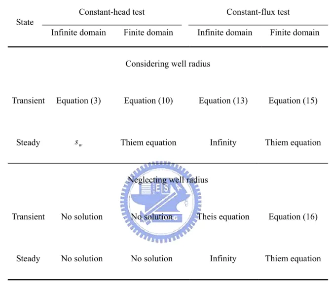
Table 1 The transient and steady-state drawdown solutions for constant-head and constant flux tests --- 42 Table 2 The boundary-effect and steady-state time criteria for the finite-domain

List of Figures

Figure 1 Schematic diagram of drawdown distribution under pumping in a confined aquifer. --- 44 Figure 2 Dimensionless wellbore flux versus dimensionless time for the

finite-domain solution, Equation (11) with R r_w = 10 and 102_{, the} infinite-domain solution, Equation (5), and the Thiem equation. Note that both Equations (5) and (11) are solved for the constant-head test. --- 45 Figure 3 Dimensionless drawdown versus dimensionless time for the finite-domain

solution, Equation (15), with R r_w = 103 and 104 and ₌₁₀2

w

r

r , the

infinite-domain solution, Equation (13), and the Thiem equation. Note that both Equations (13) and (15) are solved for the constant-flux test. -- 46

Notation

The following symbols are used in this dissertation:

0

I = modified Bessel function of the first kind of order zero;

0

J = Bessel function of the first kind of order zero;

1

J = Bessel function of the first kind of order one;

0

K = modified Bessel function of the second kind of order zero;

1

K = modified Bessel function of the second kind of order one;

p = Laplace dummy variable;

q = pS T ;

Q = wellbore flux for constant-head test or pumping rate for constant-flux test;

Q = Laplace domain wellbore flux or pumping rate;

r = radial coordinate;

w

r = well radius;

R = radius of influence; s = drawdown;

s = Laplace domain drawdown;

w

s = drawdown in pumping well;

S = storativity of confined aquifer;

T = transmissivity of confined aquifer;

u = r2S

( )

4Tt _; U = R2S

( )

4Tt _; W = well function;

0

Y = Bessel function of the second kind of order zero;

1

Y = Bessel function of the second kind of order one;

n α = roots of J₀(r_wα)Y₀(Rα)−Y₀(r_wα)J₀(Rα )=0; n β = roots of J₁(r_wβ)Y₀(Rβ)−Y₁(r_wβ)J₀(Rβ )=0; λ = ₄T

(

c2r_w2S

)

_{which c=exp}

( )

_{γ ;} η = λ ; t

γ = 0.57722_K is the Euler’s constant;

n

χ = roots of Bessel function J₀(χ)=0; and

Chapter 1 Introduction

1.1 Statement of the problem

The spatial and temporal distributions of drawdown in an aquifer may change in response to a head change or pumping rate applied at the test well. The former holds a fixed drawdown in the test well and is referred to the constant-head test. The latter keeps a constant pumping rate in the test well and is referred to the constant-rate test. A given drawdown solution can be used to predict the drawdown distribution at any location and time if the aquifer parameters are known. It can also be used to determine the aquifer parameters if coupled an optimization approach in analyzing the observed drawdown data.

Theis and Thiem equations are the famous transient and steady-state drawdown solutions, respectively, of a constant-rate test conducted in confined aquifer. Both equations are easily used to predict the aquifer drawdown distribution in practical application. Theis equation is derived under the conditions of having an infinite extent confined aquifer and neglecting the effect of well radius. It, therefore, is not valid if the aquifer has a finite boundary. In addition, the Theis equation will give an infinite drawdown solution if the time approaches infinity or the radius approaches zero. Chen [1984] proposed a modified Theis equation for drawdown distribution in a finite confined aquifer and gave a time criterion when applying the Theis solution.

Thiem equation, the steady-state solution, can be derived either from the continuity equation coupled with Darcy’s law [e.g., Todd and Mays, 2005] or the radial steady-state flow equation [e.g., Charbeneau, 2000]. Many researches have discussed the problem of steady-state flow and gave a warning of erroneous result when employing Thiem equation to problems of an infinite aquifer [e.g., Bear, 1979]. Zaadnoordijk [1998] proposed a superposition algorithm, includes Thiem equation and Theis equation, to simulate the transition between two given steady-state groundwater fields. His study indicates that the steady-state condition is directly related to the effects of well radius and finite boundary. However, the issue of deriving the Thiem equation directly from the transient drawdown solutions has never been addressed before.

Contrary to the constant-flux test, the constant-head aquifer test is suitable in determining the hydraulic parameters of low-permeability aquifer. This test maintains a constant head on the pumping/injection well throughout the test period, and the change of flow rate across the wellbore versus time is recorded [e.g., Batu, 1998]. The head distribution for constant-head test in a confined aquifer is analogous to the heat distribution for constant temperature maintained at a bounded circular cylinder; thus, the head solutions in both Laplace domain and time domain can be obtained from Carslaw and Jaeger [1959]. The wellbore flux can then be

derived based on the solution of head distribution and Darcy’s law [e.g., Yang and Yeh, 2002; Peng et al., 2002]. However, the time domain solution of the wellbore flux is complex and difficult to accurately evaluate. Therefore, it was common to derive the approximate solutions for small or large value of the time for the wellbore flux [e.g., Carslaw and Jaeger, 1959, p.336].

One way for obtaining the small- or large-time solution is to apply the relationship of large p versus small t (hereinafter referred to as LPST) or small p versus large t (hereinafter referred to as SPLT) to the Laplace domain solution, respectively. This concept is based on a symbolic relation between the derivative operator of time, i.e., d dt, in the time domain and the dummy variable, p, in the Laplace domain [van Everdingen and Hurst, 1949]. Then, one may obtain a small- or large-time solution from taking the inverse Laplace transform on the reduced Laplace domain solution for a large or a small dummy variable, respectively. Some of the successful illustrations of applying this concept can be found in the groundwater literature. van Everdingen and Hurst [1949] used the relationships of LPST and SPLT to derive the pressure head of groundwater flow in a reservoir at small and large time, respectively. Accounting for the aquitard storage for the flow in a leaky aquifer system, Hantush [1960] obtained the small- and large-time drawdown solutions by applying those two relationships. Neuman and Witherspoon

[1969] studied the problem for flow in a confined two-aquifer system by considering the aquitard storage and drawdown in the unpumped aquifer. They used the LPST relationship to obtain the small-time solution for their problem. Singh and Sagar [1980] proposed approximate solutions of head to the linearized flow equation of slightly compressible fluids by using the relationships of LPST and SPLT. Javandel and Witherspoon [1983] and Butler and Liu [1993] provided a large-time solution for pumping-induced drawdown in a vertical and horizontal nonuniform aquifer, respectively, based on the SPLT relationship. Chakrabarty et al. [1993] provided a nonlinear pressure distribution of compressible liquid and the corresponding small- and large-time solutions obtained in a homogeneous formation using the relationships of LPST and SPLT, respectively. In addition, a number of approximate solutions at small and/or large time were derived based on these relationships in areas such as the solute transport problem [van Genuchten et al., 1984; Chen, 1985; 1986; Yates, 1990], dual-porosity media problem [Barker, 1985], and unsteady infiltration problem [Philip, 1986].

However, Chen and Stone [1993] presented a calculation of the flow rate across the wellbore for the constant-head test problem and concluded that the SPLT relationship might fail to obtain a correct large-time solution in this case. Later, Mathias and Zimmerman [2003] indicated that a poor result was obtained by Gerke

and van Genuchten [1993] when using the relationship of small p versus large t to derive the water transfer coefficient for the dual-porosity media problem. The relationships of LPST and SPLT have been widely used in the groundwater literature for more than 40 years. Previous researches indicated that the SPLT relationship could successfully yield correct large-time solutions if applied to the related Laplace domain solutions. The contrary results of Chen and Stone [1993] and Mathias and Zimmerman [2003], therefore, may depress the further study on this issue.

1.2 Objectives

The drawdown distribution may change in response to the constant-head or the constant-flux test. Mathematically, these two tests can be formulated as different types of boundary value problem. With or without considering the effect of well radius, many studies have been devoted to developing analytical solutions for those problems under various boundary conditions. The goal of this dissertation is to investigate the problems regarding to the drawdown solutions of constant-head and constant-flux tests in a homogeneous confined aquifer. Toward this goal the dissertation organization is as follows:

(1) To examine the drawdown solutions of constant-head and constant-flux tests in a finite or infinite confined aquifer with or without the consideration of the effects of

well radius;

(2) To verify the drawdown solutions of these two tests in a finite domain converging to the Thiem equation after a long period of pumping;

(3) To present dimensionless time criteria required to approximate the solutions of finite domain by the infinite-domain solution or the Thiem equation;

(4) To resolve the dispute on the validity of the SPLT relationship raised by Chen and Stones [1993] and Mathias and Zimmerman [2003] through the detailed mathematical development; and

(5) To derive a correct large-time solution of the wellbore flux rate for the constant-head test based on the Laplace domain solution and the SPLT relationship.

Chapter 2 Drawdown Solutions for Constant-head Test

This chapter considers the constant-head test conducted in a homogeneous, isotropic confined aquifer of constant thickness as shown in Figure 1. The one-dimensional radial flow equation describing the drawdown in a confined aquifer can be written as [Batu, 1998, p.147]

t s T S r s r r s ∂ ∂ = ∂ ∂ + ∂ ∂ 1 2 2 (1)

where s ,

( )

r t is the observable drawdown corresponding to the radial distance r from the test well and the time variable t, S is the storativity, and T is the transmissivity. The drawdown is initially assumed zero before an aquifer test, i.e.,

( )

r,0 =0

s .

For the constant-head test, the drawdown in the test well is maintained a constant and denoted as s_w. The rim of the wellbore is selected as the inner boundary and the inner boundary condition for the drawdown is then denoted as s

( )

r_w,t =s_w where

rw is the well radius. An outer boundary condition should be provided for solving the flow equation, Equation (1). Hereinafter, this study will present and discuss the solution for the outer boundary specified as a zero drawdown and located at either an infinite or a finite distance from the test well. In addition, the drawdown solution derived by considering or neglecting the effect of the well radius will also be

presented.

2.1 Infinite domain with a finite well radius

Analytical solution

It is assumed that the outer boundary is located at infinity and the outer boundary condition is expressed as s

( )

∞ t, =0. The solution subject to the infinite domain assumption is referred to as an infinite-domain solution. By using the method of Laplace transforms, the general Laplace domain solution of Equation (1) can be obtained in terms of bases I₀ and K₀, which are modified Bessel functions of the first and second kinds of order zero, respectively. The function I₀ tends to infinity under the outer boundary condition and therefore must be excluded.

Application of the inverse Laplace transform under the inner boundary condition yields the Laplace domain and time domain drawdown distribution for the constant-head test, respectively, as [Carslaw and Jaeger, 1959, p.335]

( )

) ( ) ( , 0 0 w w qr K qr K p s p r s = (2) and

( )

( ) ( )

( ) ( )

_      + −      − − =

∫

∞ x dx x r Y x r J x r Y rx J x r J rx Y t x S T s t r s w w w w w ) ( ) ( exp 2 1 , ₂ 0 2 0 0 0 0 0 0 2 π (3)

where p is the Laplace variable; q= pS T ; K₁ is modified Bessel function of the second kind of order one; and J₀ and Y₀ are the Bessel functions of the first and second kinds of order zero, respectively.

The flow rate across the wellbore at the test well, therefore, can be obtained by applying Darcy’s law to Equations (2) and (3). Accordingly, the wellbore fluxes for Laplace domain and time domain are, respectively,

(

)

) ( ) ( 2 , 0 1 w w w w w qr K qr K q p s T r p r Q = π (4) and

( )

x dx x r Y x r J t x S T Ts t r Q w w w w ) ( ) ( 1 exp 8 , ₂ 0 2 0 0 2 +      − =

∫

∞ π (5)

Note that the negative sign of Q corresponds to withdrawal and the positive sign corresponds to injection.

Because the exponential term on the right-hand side of Equation (3) reduces to zero as time approaches infinity; thus, the steady-state drawdown is obtained as s_w. This result implies that the steady-state drawdown within the entire domain is kept the same as the fixed drawdown at test well. Also, Equation (5) shows that the wellbore flux decreases with the increasing time and approaches zero at the large time rather different from the Thiem equation. These results suggest that under the infinite outer

boundary condition there is not enough water to maintain a constant non-zero flow rate within the aquifer for the constant-head test. The solid line in Figure2 demonstrates the plot of dimensionless wellbore flux of Equation (5),

( )

rw t Tsw

Q , 2π , versus dimensionless time, Tt r_w2S_{. It can be observed that the}

wellbore flux approaches zero as time becomes infinitely large.

Approximate solution at large time

The time domain solution of the wellbore flux, Equation (5), is complicate and difficult to evaluate accurately due to the problems of alternately oscillatory, slowly convergence, and a singularity at the origin [Peng et al., 2002]. Therefore, it is common to derive a large-time approximate solution of the wellbore flux by using the SPLT relationship. However, Chen and Stone [1993] and Mathias and Zimmerman [2003] indicate that erroneous results were obtained when applying the SPLT relationship. Based on SPLT, the approximate solution for large-time drawdown distribution of constant-head test under the assumptions of an infinite domain and a well of a finite radius can be derived successfully and is presented as follows. In addition, a detailed mathematical derivation using SPLT approach for deriving the water transfer coefficient involved in Mathias and Zimmerman [2003] is shown in Appendix A.

Using the limiting forms of K₀

( )

x ≅−

[

ln

( )

x 2 +γ

]

and K₁

( )

x ≅1 x, where K 57722 . 0 =

γ is Euler’s constant, for small value of x [Abramowitz and Stegun,

1970, p.375], the wellbore flux for small p, Equation (4), in Laplace domain can be

reduced to

(

)

₍

₎

λ π p p Ts p r Q _{w w} ln 1 4 , ≅− (6)

where _{λ =4}T

(

c2r_w2S

)

_{and c=exp}

( )

_{γ . The large-time wellbore flux is}

subsequently obtained by taking the inverse Laplace transform of Equation (6). Chen and Stone [1993] used a inverse Laplace transform formula given by the Oberhettinger and Badii [1973] (formula 6.75, p.276 and 424) for the inverse Laplace transform of term 1

[

p ln

(

p λ

)

]

in Equation (6) as

(

)

∫

( )

(

)

∞ − + Γ =       0 1 1 ln 1 dx x t p p L x λ λ (7)

where Γ

( )

x is the gamma function. They integrated Equation (7) and obtained the large-time wellbore flux as Q(r_w,t)=−∞. In addition, they showed that this large-time wellbore flux was contradictory to the result obtained by applying the Tauberian theorem (also called final-value theorem [Spiegel, 1965]) to Equation (6), i.e., 0Q(r_w,t→∞)= . Based on their study, they concluded that the application of the SPLT relationship should be used with care because of possible failure to obtain a

correct large-time solution.

In fact, the use of inverse Laplace transform formula of Equation (7) should be under a constraint of p>

λ

which is proven in the Appendix A. For most confined aquifers, the value of the storativity falls in the range 10-5 _{~ 10}-3 _{and for sand and silt} formations the value of hydraulic conductivity falls in the range of 10-2 _{~ 10}1 _m/day [Todd and Mays, 2005, p.93]. Assuming that the thickness of confined aquifer is 10 m and the radius of the test well is 5 cm; then, the value of λ ranges from 104/day to 109_{/day. Notice that the Laplace variable p is required to be small in Equation (6)} and λ should be small too. Yet, the value of λ is larger than 104/day in reality as demonstrated above; accordingly, Equation (7) does not hold at all.

Hereafter, this study proposes an alternative formula for the inverse Laplace transform of term 1

[

p ln

(

p λ

)

]

in Equation (6). Ritchie and Sakakura [1956] presented an article on expanding the solutions of the heat conduction equation in terms of an infinite series approximately in an internally bounded cylindrical solid. They gave the inverse Laplace transform for the term 1

[

p ln

(

p λ

)

]

when p is small as

(

)

∑

=

(

)

₌ + −               − Γ      −       − =       N s s s s d d s p p L 0 ₀ 1 1 1 1 1 ln 1 ln 1 ν ν ν η λ (8)

coefficient, and N is the number of truncated terms depending on the values of the

remainder.

The right hand side (RHS) of Equation (8) is a summation of products of the dimensionless variable ln and the constant value of the Gamma function. For a η large value of time, the terms of 1

( )

lnη 5 and higher order terms may be truncated since η is proportional to the dimensionless time. Therefore, the large-time wellbore flux can be obtained based on Equations (6) and (8). Appendix B shows the detailed expansion of Equation (8) and the large-time solution for the wellbore flux is obtained approximately as

( )

( )

( )

( )

( )

            + − − − + − ≅ ₄ 2 3 3 2 2 2 _ln 3 2 2 ln 6 ln ln 1 4 , η ξ γ π γ η π γ η γ η π _w w t Ts r Q (9)

The numerators of the RHS terms of Equation (9) are all constants and the denominators are the function of dimensionless time, _η=4Tt

(

c2r_w2S

)

_{. The value of}

η

ln reaches infinity if t approaches infinity; therefore, Equation (9) becomes zero, i.e., the steady-state solution for the wellbore flux is zero. Notice that Jaeger [1943] and Carslaw and Jaeger [1959, p.336] gave a large-time wellbore flux which has the first three terms and first two terms of Equation (9), respectively.

2.2 Infinite domain with neglecting the well radius

For the case of neglecting the effect of test well radius, that is, r_w→0, the basis

0

K of the general Laplace domain solution tends to infinity and therefore there is no

solution for this case. The transient and steady-state solutions of the drawdown for the constant-head test with and without considering the effect of well radius under the infinite domain assumption are listed in Table 1.

2.3 Finite domain with a finite well radius

In this section, a well of a finite radius is considered and a finite distance, R, is

selected to represent the outer boundary if the drawdown beyond R is zero or negligible. Generally speaking, the radius of influence which can be estimated by an empirical relationship [Bear, 1979, p.306] is finite. Thus, the solution under a finite outer boundary condition denoted as s

( )

R,t =0 is referred to as a finite-domain solution. Carslaw and Jaeger [1959, p.332] gave the solution for this problem under Cauchy boundary conditions. By assuming the flux of the Cauchy boundary being equal to zero, a new drawdown solution for an aquifer of a finite domain under the assumption of a finite well radius can be derived as

( )

₍

( )

₎

_[

_]

_      − −      − − =

∑

∞ =1 02 2 0 2 0 0 0 0 0 2 ) ( ) ( ) ( ) ( ) ( ) ( ) ( exp ln ln , n w n n n n n w n n w n w w R J R J r J r J r Y r Y r J t S T r R r R s t r s α α α α α α α α π (10)

where α_n are the roots of J₀(r_wα)Y₀(Rα)−Y₀(r_wα)J₀(Rα )=0 . A detailed derivation for Equation (10) is given in Appendix C. The flow rate at wellbore can then be determined as

( )

_[

(

_]

)

_      − − + =

∑

∞ =1 02 2 0 2 0 2 ) ( ) ( ) ( exp 4 ln 2 , n w n n n n w w w R J R J r J S t T R r s T t r Q α α α α π (11)

Obviously, the steady-state wellbore flux of Equation (11) for time approaching infinity is Q

( )

r_w =2πTs_w ln

(

R r_w

)

which indeed is the Thiem equation. Figure 2 shows that the curve of Equation (11), i.e., the finite-domain solutions, coincides with that of Equation (9), i.e., the infinite-domain solutions, at the early stage of the pumping test and asymptotically approaches Thiem equation after a long period of time. In other words, the infinite-domain solution can approximate the finite-domain solution when time is less than the boundary-effect time criterion, denoted as t₁, implying that the finite boundary has no affect on the wellbore flux. In addition, the finite-domain solution can be reduced to Thiem equation when time is larger than the steady-state time criterion, denoted as t₂, implying that the wellbore flux can be considered at the steady state. It is worth noting that both the Thiem equation and the infinite-domain solution has the advantage of computing the drawdown solution more easily over the finite-domain solution.

w

r

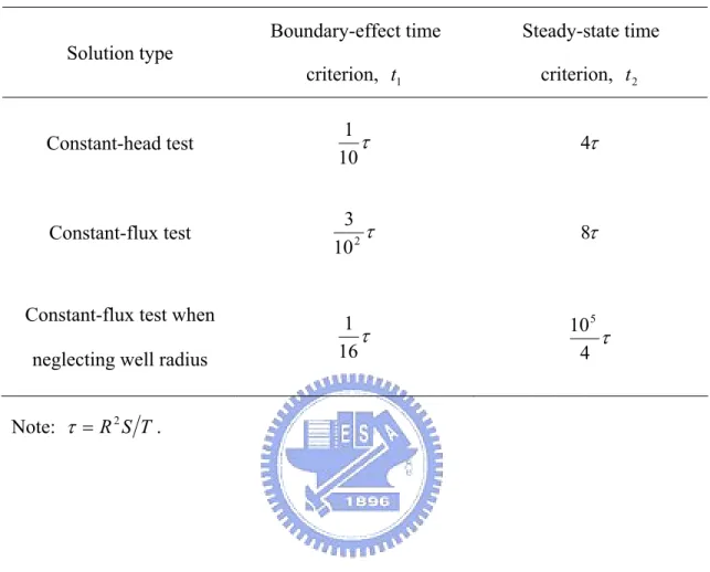
R . The time criteria of t₁ and t₂can be obtained as R2S 10T _{and 4R}2_{S T,}

respectively, for the constant-head test where the absolute difference of dimensionless wellbore flux between Equations (9) and (11) is about less than ₁₀−5_{. Table 2 gives}

a list of time criteria for the finite-domain solution.

2.4 Finite domain with neglecting the well radius

In this section, the outer boundary of radial flow system is located at finite distance from the test well and the inner boundary of well radius is negligible. Note that I and ₀ K are the bases of the general Laplace domain drawdown solution for ₀

the constant-head test as mentioned in section 2.1. Therefore, the base K has to ₀

be excluded from the general solution as r_w →0 and the other base I can not ₀

satisfy the boundary conditions of fixed drawdown at wellbore and zero drawdown at the finite distance simultaneously. Therefore, there is no solution for this case. Table 1 also lists the transient and steady-state drawdown solutions of the constant-head test when the outer boundary is finite with and without considering the effect of well radius.

Chapter 3 Drawdown Solutions for the Constant-flux Test

This chapter considers a constant-flux test conducted at a confine aquifer. Equation (1) is the one-dimensional radial flow equation describing the drawdown distribution. The initial condition for the drawdown before pumping is assumed zero. The drawdown solutions are presented in the following sections for the cases of the outer boundary of zero drawdown located at either an infinite or a finite domain with or without considering the effect of the inner boundary of well radius.

3.1 Infinite domain with a finite well radius

The constant-flux test at a constant pumping rate, says Q, is conducted at the test

well. Thus, the inner boundary condition for the constant-flux test may be written as

T r Q r s w r r w 2π − = ∂ ∂ = (12)

The drawdown solution for the constant-flux test subject to Equation (12) and zero drawdown at infinity can be obtained by the application of the Laplace transforms as [Carslaw and Jaeger, 1959, p.338]

( )

_∫

∞ + −            − − = 0 2 2 1 2 1 1 0 1 0 2 2 _{( ) ( )} ) ( ) ( ) ( ) ( exp 1 , x dx x r Y x r J x r Y rx J x r J rx Y t x S T T r Q t r s w w w w w π (13)

numerical evaluations for a radial two-zone drawdown equation for groundwater under constant-flux pumping in a finite-radius well. Their solution reduces to Equation (13) if the transmissivities and storativities for the skin zone and formation zone are the same.

Figure 3 gives a graphical representation of dimensionless drawdown of Equation (13) for the dimensionless time ranging form _{10 to} 2 _{10 . The plot of} 9

drawdown distribution demonstrated that the drawdown increases with time and diverges as time approaches infinity. It implies that there is not enough water at the outer boundary to balance the continuous well pumping and the aquifer is overdrawdown when time goes infinitely large. This result indicates that the steady-state drawdown solution of the constant-flux test in an infinite domain by considering the effect of the well radius does not reduce to the Thiem equation.

3.2 Infinite domain with neglecting the well radius

The solution for the constant-flux test neglecting the effect of well radius conducted in an infinite domain is analyzed in this section. By applying the Laplace transforms and the asymptotic form of modified Bessel function [Abramowitz and Stegun, 1970], one obtains the drawdown equation as

( )

( )

dx x x T Q t r s u

∫

∞ ₋ = exp 4 , π (14)

where u₌r2S

( )

4Tt _{is inversely proportional to time.}

Equation (14) is the famous Theis equation. The integration in Equation (14) is called the well function and expressed as W

( )

u which tends to infinity when time approaches infinity. Thus the drawdown of the Theis equation becomes infinity. In addition, Cooper-Jacob's solution, a special case of the Theis equation under the condition of u<0.01, should also give an infinite drawdown solution when u approaches zero.

The transient and steady-state drawdown solutions for a constant-flux test conducted in an aquifer with an infinite outer boundary are compared in Table 1. The results for the constant-head and constant-flux tests indicate that these two tests in an infinite domain do not have steady-state solutions; thus, Equations (3), (13), and Theis equation can not reduce to the Thiem equation.

3.3 Finite domain with a finite well radius

Similar to the development of Equation (10), the drawdown solution for Equation (1) subject to Equation (12) and a zero drawdown at finite distance can be obtained as [Carslaw and Jaeger, 1959, p.334]

( )

_[

_]

        − −      − − =

∑

∞ =1 02 2 2 1 0 1 0 1 2 ) ( ) ( ) ( ) ( ) ( ) ( ) ( exp ln 2 , 0 n n w n n n n n w n n w n w J r J R J R r J r Y r Y r J t S T r r R T Q t r s β β β β β β β β β π π (15)

where β_n represent the roots of J₁

( ) ( )

r_wβ Y₀ Rβ −Y₁

( ) ( )

r_wβ J₀ Rβ =0 . The steady-state drawdown solution can be easily obtained by setting the time to be infinity in Equation (15) which is indeed the Thiem equation if the distance r is

equal to the well radius.

Figure 3 shows the distribution of dimensionless drawdown of Equation (15) versus dimensionless time for R r_w equal to 103 and 104 with ₌₁₀2

w

r

r . It also demonstrates that the curve of Equation (15), i.e., finite-domain solutions, can be approximated by that of Equation (13), i.e., infinite-domain solutions, at early period of time and reduce to Thiem equation at a large period of time. The former indicates the drawdown solution can be treated as that for an infinite aquifer before the boundary effect acts. The latter implies that the drawdown almost reaches its steady-state solution and the Thiem equation is applicable if the time is larger than the steady-state time criterion. When the absolute difference of dimensionless drawdown is less than ₁₀−5_{, the dimensional time criteria of}

1

t and t₂ for the constant-flux test considering well radius are 3R2S 100T _{and 8R}2_{S T ,}

3.4 Finite domain with neglecting well radius

In this section, the outer boundary is some finite distance away and the well radius is negligible. Chen [1984] obtained the drawdown solution for this case as

( )

=

[

( )

−

( )

+2Φ

]

4 , W u W U T Q t r s π (16) and

(

)

[

]

( )

∫

(

)

∑

      − − − ⋅ = Φ ∞ = 1 0 2 1 1 2 1 0 4 1 exp x dx U x x U J U u J _n n n n n χ χ χ χ (17) where U is R2S

( )

4Tt _and n

χ represents the roots of Bessel function J₀(χ_n)=0. Both the arguments u and U in Equation (11) are inversely proportional to time. The functions W(u) and W(U) can be expressed in terms of an infinite series and approximated as −

(

0.5772+lnu

)

and −

(

0.5772+lnU

)

, respectively, as u→0 and U →0 after a large period of time [Todd and Mays, 2005, p.167]. The difference of W(u) and W(U) reduces to 2ln

( )

R r where r is a finite distance from the test well. Moreover, the exponential term in the integrand of Equation (17) approaches zero as U →0 and the value of Φ is negligible. As a result, the drawdown of Equation (16) approaches Thiem equation when time approaches infinity. The results of transient and steady-state drawdown solutions of the constant-flux test under a finite outer boundary condition by considering or neglecting

the effect of well radius are also shown in Table 1.

Again, Equation (16), i.e., a finite-domain solution, can be approximated by the Theis equation, Equation (14), when U ≥4 [Chen, 1984] and reduce to the Thiem equation when _{U ≤10}−5 _{if the absolute difference of dimensionless drawdown is less}

than ₁₀−5_{. The time criteria of} 1

t and t₂ for the constant-flux test by neglecting the effect of well radius are R2S 16T _{and 10}5_R2_{S 4T, respectively, as shown in}

Chapter 4 Conclusions

The uses of the drawdown solution in predicting the drawdown distribution or determining the formation properties have been intensively studied in hydrology literature. Two well-known tests, the constant-head and constant-flux tests, are routinely used toward those goals. However, the derivations from the transient-state solution to the Thiem equation and the approximate solution at large period of time obtained from Laplace domain solution have not ever been thoroughly or correctly studied. Two main contributions from this dissertation can be summarized as follows.

First, the steady-state solutions developed from transient drawdown solutions for constant-head and constant-flux tests in a finite or infinite domain and with or without considering the effect of well radius have been presented. A new transient drawdown solution is derived for the constant-head test by considering the effect of well radius and maintaining a zero drawdown at a finite boundary. The results show that the finite domain condition is necessary for obtaining a steady-state solution from a transient solution for a groundwater flow problem. Such an imposed condition ensures that the mass balance is satisfied and the flow can reach steady state condition within a bounded domain. In addition, the time criteria are provided for the approximation of the finite-domain solution by the infinite-domain solution or Thiem

equation. The infinite-domain solutions can be used to determine the drawdown distribution or the aquifer parameters if the time is smaller than the boundary-effect time criterion. Similarly, the Thiem equation is valid if the time is greater than the steady-state time criterion.

Second, in regard to the large-time solution of wellbore flux in constant-head problem, this study found that the inverse Laplace transform formula in Oberhettinger and Badii [1973] adopted to invert Laplace domain solution by Chen and Stone [1993] should be under the constraint p>

λ

. One will obtain an erroneous solution if applying that inverse Laplace transform formula without satisfying this necessary constraint. Therefore, the inconsistent results obtained by Chen and Stone [1993] from the SPLT relationship and the Tauberian theorem that arose from a violation of the constraint from applying the inverse Laplace transform formula rather than using the SPLT relationship. In addition, a new large-time solution of the wellbore flux for the constant-head test is presented based on the SPLT relationship and the work of Ritchie and Sakakura [1956].

References

Abramowitz, M., and I.A. Stegun (1970), Handbook of Mathematical Functions, Dover Publications, New York.

Barker, J.A. (1985), Block-geometry functions characterizing transport in densely fissured media, J. Hydrol., 77, 263-279.

Batu, V. (1998), Aquifer Hydraulics, John Wiley, New York.

Bear J. (1979), Hydraulics of groundwater, McGraw-Hill, New York.

Butler, J.J., Jr., and W. Liu (1993), Pumping tests in nonuniform aquifers: The radially asymmetric case, Water Resour. Res., 29, 259-269.

Carslaw, H.S., and J.C. Jaeger (1959), Conduction of Heat in Solids, 2nd ed., Oxford University Press, London.

Charbeneau R.J. (2000), Groundwater hydraulics and pollutant transport, Prentice Hall, New York.

Chakrabarty, C., S.M.F. Ali, and W.S. Tortike (1993), Analytical solutions for radial pressure distribution including the effects of the quadratic-gradient term, Water

Resour. Res., 29, 1171-1177.

Chen C.S. (1984), A reinvestigation of the analytical solution for drawdown distributions in a finite confined aquifer, Water Resour. Res., 20, 1466-1468. Chen, C.S. (1985), Analytical and approximate solutions to radial dispersion from an

injection well to a geological unit with simultaneous diffusion into adjacent strata,

Water Resour. Res., 21, 1069-1076.

Chen, C.S. (1986), Solutions for radionuclide transport from an injection well into a single fracture in a porous formation, Water Resour. Res., 22, 508-518.

Chen, C.S., and W.D. Stone (1993), Asymptotic calculation of Laplace inverse in analytical solutions of groundwater problems, Water Resour. Res., 29, 207-210. Crank, J. (1956), Mathematics of Diffusion, Oxford Univ. Press, New York.

Doetsch, G. (1961), Guide to the Applications of Laplace Transforms, Van Nostrand Reinhold, New York.

Dykhuizen, R.C. (1990), A new coupling term for dual-porosity models, Water Resour.

Res., 26, 351-356.

Gerke, H.H., and M.T. van Genuchten (1993), Evaluation of first-older water transfer term for variably saturated dual-porosity flow modes, Water Resour. Res., 29, 1225-1238.

Hantush, M.S. (1960), Modification of the theory of leaky aquifers, J. Geophys. Res.,

65, 3713-3725.

Jaeger, J.C. (1943), Heat flow in the region bounded internally by a circular cylinder,

Proc. Roy. Soc. Edinburgh, 61, 223-229.

penetrating well in a two-layer aquifer, Water Resour. Res., 19, 567-578.

Mathias, S.A., and R.W. Zimmernan (2003), Laplace transform inversion for late-time behavior of groundwater flow problems, Water Resour. Res., 39, 1283, doi: 10.1029/2003WR002246.

Neuman, S.P., and P.A. Witherspoon (1969), Theory of flow in a confined two-aquifer system, Water Resour. Res., 5, 803-817.

Oberhettinger, F., and L. Badii (1973), Tables of Laplace Transforms, Springer-Verlag, New York.

Peng, H. Y., H. D. Yeh, and S. Y. Yang (2002), Improved numerical evaluation for the radial groundwater flow equation, Adv. Water Resour., 25, 663-675.

Philip, J. R. (1986), Linearized unsteady multidimensional infiltration, Water Resour.

Res., 22, 1717-1727.

Ritchie, R.H., and A.Y. Sakakura (1956), Asymptotic expansions of solutions of the heat conduction equation in internally bounded cylindrical geometry, Appl. Phys.,

27, 1453-1459.

Singh, S.R. and B. Sagar (1980), On Jacob’s approximation in flow through porous media, Water Resour. Res., 16, 377-380.

Spiegel, M.R. (1965), Theory and Problems of Laplace Transforms, Schaum Pub. Co., New York.

Todd, D.K., and L.M. Mays (2005), Groundwater Hydrology, John Wiely & Sons. van Everdingen, A.F., and W. Hurst (1949), The application of the Laplace

transformation to flow problems in reservoirs, Trans. Am. Inst. Min. Metall. Eng.,

186, 305-324.

van Genuchten, M.T., D.H. Tang, and R. Guennelon (1984), Some exact solutions for solute transport through soils containing large cylindrical macrospores, Water

Resour. Res., 20, 335-346.

Yang, S.Y., and H.D. Yeh (2002), Solution for flow rates across the wellbore in a two-zone confined aquifer, J. Hydraulic Eng. ASCE, 128, 175-183.

Yates, S.R. (1990), An analytical solution for one-dimensional transport in heterogeneous porous media, Water Resour. Res., 26, 2331-2338.

Yeh H.D., S.Y. Yang, H.Y. Peng (2003), A new closed-form solution for a radial two-layer drawdown equation for groundwater under constant-flux pumping in a finite-radius well, Adv. Water Resour., 26, 747-757.

Zaadnoordijk W.J. (1998), Transition from transient Theis wells to steady Thiem wells, Hydrological Sciences J, 43, 859-873.

Appendixes

Appendix A: Examination of SPLT for dual-pore problem Appendix B: Derivation of Equation (7)

Appendix C: Derivation of Equation (9) Appendix D: Derivation of Equation (10)

Appendix A: Examination of SPLT for dual-pore problem

A fractured aquifer consisted of fractures, fissures, cracks, and macropores can be simulated as two separate but connected medium, one is associated with fracture medium and the other involves porous matrix. Such a fractured aquifer system is called dual-porosity system. Mathematically, a dual-porosity system involves two flow equations which are coupled by means of a transfer term of water flow [Dykhuizen, 1990]. Gerke and van Genuchten [1993] proposed a first-order model to account this transfer term which is assumed to be proportional to the difference in pressure head between the fracture medium and porous matrix. The specific value of water transferred to head difference is referred as water transfer coefficient.

For the dual-porosity media problem, Gerke and van Genuchten [1993] solved a large-time water transfer coefficient by comparing two Laplace domain solutions, one was the “first-order” flux equation between fracture and matrix and the other was Richards’s equation within the matrix block, while p became small. Moreover, Mathias and Zimmerman [2003] also obtained a large-time water transfer coefficient for the dual-porosity media problem based on the time domain approach. Their solution differs from the one obtained by Gerke and van Genuchten [1993] using the Laplace domain approach based on the SPLT relationship. When comparing both Laplace- and time domain solutions with the exact solution, they implicitly indicated

that the SPLT relationship did not hold. Therefore, the following context will go through the detailed mathematical derivations involved in the issues of Gerke and van Genuchten [1993] and resolve the argument on the validity of the SPLT relationship.

If the pressure head of the fracture pore is considered to be a constant in time, the water transfer coefficient can be obtained by comparing two rearranged flow equations in Laplace domain as [Gerke and van Genuchten, 1993]

( )

( )

p h p h h p h f mi mi m , , tanh ₊       − = ξ ξ (A1) and

( )

_      + +       + = , ₋₁ 1 1 1 1 ζ ζ p h p h p h f mi m (A2)

where h_m and h_m,i are the Laplace domain head and the initial head, respectively, in the matrix block; h is the imposed head at the fracture boundary; and variables _f

(

)

[

]

0.5

1 w_f C_mp K_a

a −

=

ξ and ζ = 1

(

−w_f

)

C_mp α_w while a is the characteristic half width of the matrix block, w is the fracture porosity, _f K is the hydraulic _a conductivity of the matrix block near the fracture/matrix interface, C is the specific _m water capacity at the matrix, and α_w is the water transfer coefficient.

formula of Doetsch [1961] when time is large. Based on the time domain approach, they obtained an exact large-time water transfer coefficient of

) 47 . 2 ( 4 2 2 2_{K a K a} a a w =π ≅

α which differs from the Laplace domain approach of

2

3K_a a

w =

α obtained by Gerke and van Genuchten [1993] derived from Equations (A1) and (A2) based on the SPLT relationship.

Once the water transfer coefficient is obtained, the normalized head difference for large value of time is [Mathis and Zimmerman, 2003]

( )

        − − = − − m f w f i m f m C w t h h h t h ) 1 ( exp , α (A3)

where h is the time domain head. Equation (A3) can be verified by comparing it _m

with the exact solution given in Crank [1956, p.48] which was shown in Mathis and Zimmerman [2003] as

( )

(

)

( )

(

)

∑

∞ =         − + − + = − − 0 2 2 2 2 2 , 2 (1 ) 1 2 exp 1 2 1 8 n _{f m} a f i m f m C w a t K n n h h h t h π π _(A4)

It is clear that the normalized head difference approaches zero while dimensionless time K_at

[

( )

2a 2(1−w_f)C_m

]

on the RHS of Equation (A4) goes to a very large value.

from the time domain approach and Laplace domain approach arises from the use of the SPLT relationship. However, this study finds that this relationship is indeed correct and the defect in Gerke and van Genuchten [1993] is mainly caused by ignoring the convergent requirements of series expansion for Equations (A1) and (A2).

Gerke and van Genuchten [1993] expanded tanh

( )

ξ and 1

(

1+ζ

)

in Equations (A1) and (A2) in terms of a series, respectively. Those two equations were then respectively expressed as

( )

(

)

(

)

(

)

(

)

(

)

(

)

        − − + − − − +         + − − − + − − = K K 3 3 3 3 6 2 2 2 2 4 2 , 3 3 3 3 6 2 2 2 2 4 2 315 1 17 15 1 2 3 1 315 1 17 15 1 2 3 1 1 a m f a m f a m f i m a m f a m f a m f f m K p C w a K p C w a K p C w a p h K p C w a K p C w a K p C w a p h p h (A5) and

( )

(

)

(

)

(

)

(

)

(

)

(

)

        − − + − − − +         + − − − + − − = K K 3 3 3 3 2 2 2 2 , 3 3 3 3 2 2 2 2 1 1 1 1 1 1 1 w m f w m f w m f i m w m f w m f w m f f m p C w p C w p C w p h p C w p C w p C w p h p h α α α α α α (A6)

The water transfer coefficient can then be obtained as _{3K a}2

a w =

α if one

and fourth terms are _{15 2K a}2 a w = α ( 2.74_{K a}2) a ≅ and _{3 31517K a}2 a w = α ) 65 . 2 ( _{K a}2 a

≅ , respectively. It seems that the estimated water transfer coefficient appears monotonously decreasing from 3 and asymptotically approaches to 2.47. Notice that Gerke and van Genuchten [1993] truncated the third and remaining higher order terms of p in Equations (A5) with (A6) because of small p.

In fact, the series expansion for tanh

( )

ξ in Equation (A1) and 1

(

1+ζ

)

in Equation (A2) should be restricted to the convergent criteria ξ <π 2 and ζ <1 [Abramowitz and Stegun, 1970, p.15 and 85], respectively. The series expansion of

( )

ξ

tanh in Equation (A1) can be expressed as [Abramowitz and Stegun, 1970, p.85]

(

)

( )

2 ! ..., 1,2,K 1 2 2 ... 315 17 15 2 3 tanh _{= −} 3 ₊ 5 ₋ 7 _{+ +} 2 2 − 2 2 −1 _{+ n=} n B _{n n} n n ξ ξ ξ ξ ξ ξ (A7)

where B_2n is the nth Bernoulli number and the convergent criterion of tanh

( )

ξ is 2

π

ξ < . Subsequently, one uses the Fourier expansion of the Bernoulli number [Abramowitz and Stegun, 1970, p.805] and obtains

( ) ( )

( )

2 1 , 1,2,... ! 2 2 1 1 2 2 1 2 = − =

∑

∞ = − n k n B k n n n n _π (A8)

Therefore, the nth term of water transfer coefficient is obtained by letting Equation (A5) equal to Equation (A6) as

( ) ( )

(

)

₍

₎

K , 2,3,... 1 2 2 K 1 2 2 ! 2 1 2 1 1 1 2 1 2 2 2 1 1 2 2 2 1 , =             − =       − − = − ∞ = + − −

∑

_k a n a B n _a n k n n n a n n n n n n w π α (A9)

The limit of α_w for n→∞ is

(

)

2 2 2 1 1 1 2 1 2 2 _K 4 K 1 2 2 lim a a k a a n k n n n n w π π α =             − = − ∞ = + ∞ →

∑

(A10)

where the limit of Riemann Zeta function,

∑

∞₌ −

∞ → 1

2

lim _k n

n k , equals 1.

The result shows that the water transfer coefficient has to be 2_{K 4a}2

a w π

α = .

Obviously, the coefficient of _{3K a}2

a w =

α obtained from the Laplace domain approach based on the SPLT relationship is exactly the same as that of Mathias and Zimmerman [2003] derived from the time domain approach. Therefore, the dispute in the discrepancy that was calculated using Laplace domain approach by making use of the SPLT relationship and those found by working in the time domain is clearly resolved.

Appendix B: Derivation of Equation (7)

By applying the Laplace transform, the integral function of Equation (7) can be expressed as

( )

(

)

( )

(

x

)

dxdt t e dx x t L x pt x

∫

∫

∫

∞ − ∞ ∞ + Γ =       + Γ _{0 0} 0 1 1 λ λ (B1)

The RHS of (B1) is a double integral and can be rearranged as

( )

(

)

(

(

x

)

)

e

( ) ( )

pt d pt dx p p dt dx x t e pt x x x pt       + Γ = + Γ

∫

∫

∫

∫

∞ ∞ ∞ − ∞ − 0 0 0 0 1 / 1 1 λ λ (B2)

The Gamma function is defined as [Abramowitz and Stegun, 1970, p.255]

(

₊

)

₌

_∫

∞ −

Γ

0

1 e u du

x u x _(B3)

Replacing the second integral in Equation (B2) by Gamma function, the RHS of Equation (B2) after the integration gives

(

)

z x x x z x p p p dx p p = = − ∞ → ∞       − =      

∫

0 0 ln 1 1 lim 1 λ λ λ (B4)

If p>λ, the term

(

p λ

)

−z approaches to zero as z→∞, then Equation (B4) reduces to

( )

(

)

(

λ

)

λ p p dx x t L x ln 1 1 0 =       + Γ

∫

∞ (B5)

Appendix C: Derivation of Equation (9)

The first four terms of Equation (8) can be rewritten using the notation of Ritchie and Sakakura [1956] as

(

)

( ) ( ) ( )

_     + + + − =       − − − − − 4 1 , 0 3 3 1 , 0 2 2 1 , 0 1 1 , 0 0 1 ln B ln B ln B ln B ln 1 η η η η λ p p L (C1) and

( )

₍

₎

, 0,1,2,3 1 1 1 1 B 0 1 , 0 ₌       − Γ      − − = = − _s d d s s s s s ν ν ν (C2)

where the coefficient _B0,−1

s is related to the Gamma function. The selected

properties of binomial coefficient, Gamma function, and Polygamma function applied to the following derivation are, respectively, [Abramowitz and Stegun, 1970]

( )

s s 1 1 − =      − (C3)

(

−ν

)

=−νΓ

( )

−ν Γ 1 (C4) and

( )

[

( )

ν

]

ν ν ψ ν = + Γ + ln 1 1 s s s s d d d d (C5) The values of _B0,−1

( ) ( ) ( )

1 1 1 1 1 1 0 1 B0, 1 0 0 − _Γ =_Γ =     − = − _(C6)

( )

₍

₎

( )

_{( )}

γ ν ν _ν Γ =− Γ =       − Γ −      − = = − 1 1 1 1 1 1 1 B ₂' 0 1 1 , 0 1 d d (C7)

( )

₍

₎

( )

_{( )}

( )

( )

_{( )}

6 1 1 2 1 1 1 1 1 2 1 B 2 2 3 2 ' 2 " 0 2 2 2 1 , 0 2 π γ ν ν _ν Γ = − Γ + Γ Γ − =       − Γ −      − = = − d d (C8) and

( )

₍

₎

( ) ( )

( ) ( ) ( )

( )

( ) ( ) ( )

( )

( )

( )

( ) ( )

( )

3 2 2 1 1 1 1 3 1 1 1 2 2 1 1 1 1 2 1 1 1 1 1 3 1 B 2 3 6 2 2 ' 3 ' '' 4 ' '' 2 ''' 0 3 3 3 1 , 0 3 ξ γ π γ ν ν _ν − + − = Γ Γ Γ Γ − Γ Γ Γ − Γ Γ Γ Γ − Γ Γ =       − Γ −      − = = − d d (C9)

where the Riemann Zeta function ξ

( )

3 =1.2020569032.

Substituting Equations (C6) - (C9) into Equation (C1) gives

(

)

( )

( )

( )

( )

            + − − − + − − =       − 4 2 3 3 2 2 2 1 ln 3 2 2 ln 6 ln ln 1 ln 1 η ξ γ π γ η π γ η γ η a p p L (C10)

Thus, the inverse Laplace transform of Equation (6) results in Equation (9) when truncating high-order terms of Equation (8).

Appendix D: Derivation of Equation (10)

General solutions of one-dimensional radial heat conduction equation in analogy to the groundwater drawdown equation subject to Cauchy boundary condition at the edges of hollow cylinder were given in Carslaw and Jaeger [1959]. The Cauchy boundary conditions in terms of drawdown were expressed as

a r k s k r s k − = = ∂ ∂ , 3 2 1 (D1) and b r k s k r s k − = = ∂ ∂ , ' 3 ' 2 ' 1 (D2) where ' 3 ' 2 ' 1 3 2 1,k ,k ,k ,k ,k

k are constant; a and b are the radial distance of inner boundary and outer boundary in the considered region, respectively. Equations (D1) and (D2) represent the combination of the constant-head and constant-flux boundary conditions.

By using the Laplace transforms, the drawdown solutions based on Equations (D1) and (D2) is

( )

[

(

)

_{( )}

(

)

]

(

)

( )

_n n n n n n n n A F r C b J k b J k t S T A t r s α α α α α α α π 0 0 ₂ ' 2 1 ' 1 1 2 1 , exp ,  −     − − =

∑

∞ = (D3) where