應用於影音多媒體無線傳輸中的自動增益控制和訊框同步器

國 立 交 通 大 學

多媒體工程研究所

碩

士

論

文

應用於影音多媒體正交分頻多工無線傳輸中的自動增

益控制和訊框同步器

The Study of Automatic Gain Control and Frame

Synchronizer for OFDM-based Multimedia

Wireless Transmission

研 究 生 : 王鴻偉

指導教授 : 林文杰 教授

應用於影音多媒體正交分頻多工無線傳輸中的

自動增益控制和訊框同步器

The Study of Automatic gain control and Frame Synchronizer for

OFDM-based Multimedia Wireless Transmission

研 究 生：王鴻偉

Student : Hung-Wei Wang

指導教授：林文杰

Advisor :

Wen-Chieh Lin

國 立 交 通 大 學

多媒體工程研究所

碩 士 論 文

A Thesis

Submitted to Institute of Multimedia and Engineering College of Computer Science

National Chiao Tung University in partial Fulfillment of the Requirements

for the Degree of Master

in

Multimedia and Engineering July 2010

Hsinchu, Taiwan, Republic of China

摘要

在這篇論文中，我們介紹了應用在 IEEE 802.15.3c 系統中的自動增益控制 器和訊框同步器。由於經過通道後訊號能量將會產生劇烈變化，為了對抗通道所 造成的訊號能量衰竭，自動增益控制器必須週期性的對可變增益放大器作控制。 我們偵測類比數位轉換器的最大可接受範圍去避免飽和錯誤和降低量化錯誤並 且利用可適性加權值去對抗通道所造成的能量衰竭，以確保類比數位轉換器的輸 入訊號能量能保持適當且穩定。 由於序文序列已在傳送端被重新取樣，使得交錯相關特性太差無法來作符元 邊界偵測。在此提出了一個新的交錯相關方法和一些加強效能的機制，例如格狀 搜尋和最大相似來作符元邊界偵測。在 IEEE 802.15.3c 通道模型和載波頻率偏 移 200 ppm 下的模擬結果指出當雜訊比大於 6 分貝時偵測錯誤率可以小於千分之 一。

Abstract

In this thesis, we introduce automatic gain control and frame synchronization algorithm for 802.15.3c systems. Due to the big variation of received signal power under path loss and shadowing effects the AGC must periodic control the VGA for whole packet with different control scheme. We are tracking the rest range of ADC to reduce quantization noise without ADC saturation and adaptive weight to defend shadowing effects. In frame synchronizer, the training sequence has been re-sampled at transmitter such that the correlation property of conventional cross-correlation metric gets too worse to estimate the symbol boundary. A new cross-correlation metric and several enhance performance schemes such as trellis search and Maximum likelihood is applying for boundary detection. Simulations in IEEE802.15.3c channel model with a carrier frequency offset (CFO) of ±200 ppm indicate that the detection error can be less than 0.1% at SNR ≧ 6 dB.

誌謝

能完成這篇論文，首先要感謝指導教授許騰尹老師。老師有耐心的每周導引 我論文的研究方向，並適時的提出問題訓練我獨立思考，培養解決問題之能力。 老師提供了實驗室所需的設備與資源，與盡力爭取實驗室所需的工具，讓我們在 研究道路上可以順利完成。謝謝老師的教導。 感謝博班學長小賢、胖達、大洋、jason、F龍，給我許許多多的研究方向與 支援。亦特別感謝ISIP Lab所有成員，感謝書書、卉萱、于萱、貴英、阿曄、建 安，我們一起熬夜寫code，一起拼口試投影片，一起拼論文，一起拼畢業。 謝謝大家地無私互相分享知識及經驗才能順利完成這篇論文。最後感謝交通 大學提供相當良好的研究環境及家人的支持與鼓勵，讓我的碩士學業能順利的完 成。 王鴻偉 謹誌 民國九十九年九月九日

Table of Contents

摘要... i Abstract ... ii 誌謝... iii Table of Contents ... iv List of Figures ... vi Chapter 1 Introduction ... 1

Chapter 2 System assumption... 3

2.1 IEEE 802.15.3c Audio/Visual HRP mode Physical Layer Specification... 3

2.1.1 Transmitter ... 3

2.1.2 Receiver ... 4

2.1.3 AV HRP preamble format ... 4

2.2 Channel model ... 5

2.2.1 Additive White Gaussian Noise ... 5

2.2.2 Multipath ... 5

2.2.3 Path loss and dynamic shadowing ... 6

Chapter 3 Proposed Algorithm ... 9

3.1 AGC ... 9

3.1.1 Initial gain control ... 10

3.1.2 Noise gain control ... 11

3.1.3 Preamble gain control ... 11

3.1.4 Pilot gain control ... 12

3.1.5 Packet detector ... 13

3.2 Boundary detection ... 16

3.2.1 Parallel cross correlation ... 16

3.2.3 Maximum likelihood ... 19

Chapter 4 Simulation ... 24

4.1 AGC ... 24

4.2 Boundary detection ... 27

Chapter 5 Conclusion and Future Work ... 30

5.1 Conclusion ... 30

5.2 Future work ... 30

List of Figures

Fig. 2.1 IEEE 802.15.3c transmitter ... 3

Fig. 2.2 IEEE 802.15.3c receiver ... 4

Fig. 2.3 IEEE 802.15.3c packet format ... 4

Fig. 2.4 Block diagram of channel model ... 5

Fig. 2.5 IEEE 802.15.3c CM2 power delay profile ... 6

Fig. 2.6 Path loss model ... 7

Fig. 2.7 TX transmitted signal ... 8

Fig. 2.8 RX received signal ... 8

Fig. 3.1.1 Block diagram of AGC ... 9

Fig. 3.1.2 AGC flow chart ... 10

Fig. 3.1.3 Correlation power of signal and noise... 15

Fig. 3.2.1 Block diagram of boundary detection ... 16

Fig. 3.2.2 Signal separator ... 17

Fig. 3.2.3 Parallel cross correlator ... 18

Fig. 3.2.4 Trellis diagram ... 19

Fig. 3.2.5 Mean absolute error of CFO ... 20

Fig. 3.2.6 CIR acquisition ... 21

Fig. 4.1 VGA input signal ... 24

Fig. 4.2 ADC output signal ... 24

Fig. 4.3 Adjustment of VGA ... 25

Fig. 4.4 Packet loss rate ... 26

Fig. 4.5 PER of AGC for different level of shadowing effects ... 27

Fig. 4.6 Boundary error rate of different detect method ... 28

Fig. 4.7 Estimate position ... 28

Chapter 1

Introduction

OFDM (orthogonal frequency division multiplexing) is an up and coming modulation technique for transmission large amounts of digital data over radio wave; this concept of using parallel data transmission and frequency division multiplexing was drawn firstly in 1960s. Due to the high channel efficiency and low multipath distortion that make high data rate possible, OFDM is widely applied in many transmission systems, e.g. WLAN systems based on IEEE802.11 series, digital audio broadcasting (DAB) and digital video broadcasting terrestrial TV (DVB-T). However, OFDM also has its drawbacks. OFDM systems are sensitive to imperfect synchronization and non-ideal front-end effects, leading to serious degradations of system performance.

Motivation

Automatic gain control(AGC) is an important issue to precisely control the signal power of our received signals to keeping the receive signals power level at the ADC input avoid saturation errors and minimize the quantization errors from ADC. But the signal power is variation under path-loss and dynamic shadowing effects. There have been several research contributions that provide automatic gain control algorithms, [1], [2], but they are not considering dynamic shadowing effects. Dynamic shadowing effects would cause a significant loss of SNR if we used conventional AGC without any scheme to defend it.

The frame synchronization design for OFDM systems has attracted a great deal of attention from both academy and industry. Most of the proposed schemes can be grouped into two categories: auto-correlation based algorithms and cross-correlation based algorithms. Delay and correlation based algorithms utilize the repetition structure of the training sequence or the guard intervals (GI) of OFDM symbols to acquire frame synchronization [3], [4], [5], [6]. They usually are very simple and have low implementation complexity. And known preamble cross-correlation based

algorithms use the good correlation property of training sequences to achieve more precise frame synchronization [7], [8], [9]. However, compared with auto-correlation based algorithms, cross-correlation algorithms have higher computational complexity. But all of those frame synchronization algorithms is unable to applying in 802.15.3c system. The auto-correlation based algorithms are always correlate with the first STS and next STS when receive signals. But the length STS in 802.15.3c is longer than general STS in 802.11a or 802.11n. It’s cost too many preamble to do the same things if full length STS is used. And the cross-correlation based algorithm is a good choice because the correlation property of cross-correlation be exist even correlation window is smaller than the full length of STS. However conventional cross correlation metric may have a big problem that the STS re-sampled at transmitter. Although the correlation property get worse due to partial length of STS and re-sample, but many scheme of synchronization would still work e.g. packet detection. But the performance of fine symbol timing is worse because the error peak produced by cross-correlation under multipath-fading.

Objective

In this work we propose an Automatic gain control algorithm to defend the dynamic shadowing effects, and our algorithm can achieve a little degradation than with ideal AGC under shadowing effects. In order to improve the performance of boundary detection which is suffer from above problem of correlation, a new correlation metric and a Maximum likelihood function applying for boundary detection. Simulations in IEEE802.15.3c channel model with a carrier frequency offset (CFO) of ±200 ppm indicate that the detection error can be less than 0.1% at SNR ≦ 6 dB

Organization

The rest of this paper is organized as follows. In Chapter 2, a brief introduction states the system description and system model. Chapter 3 describes the proposed automatic gain control and frame synchronizer. Chapter 4 shows and discusses the results. Conclusions are finally drawn in Chapter 5.

Chapter 2

System assumption

This chapter is going to describe complete simulation environments form OFDM specification of IEEE 802.15.3c Audio/Visual HRP mode PHY layer which operate at 60GHz band with 1.76GHz bandwidth and channel model.

2.1 IEEE 802.15.3c Audio/Visual HRP mode Physical Layer

Specification

2.1.1 Transmitter

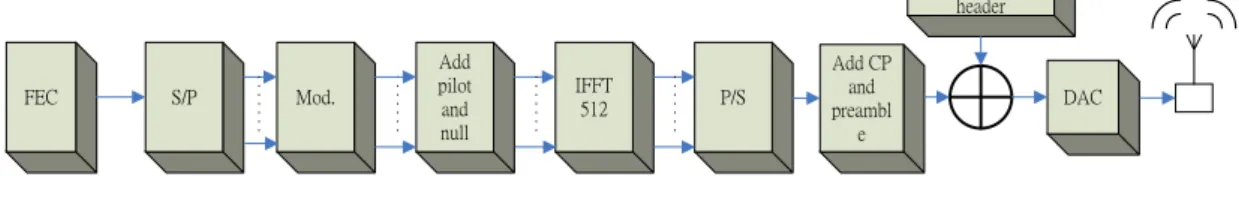
The transmitter block diagram in IEEE 802.15.3c proposal is shown as Fig. 2-1. The source data is first scrambled to prevent a succession of zeros or ones, and then it is encoded by convolution encoder with EEP coding mode, which is used as Forward Error Correction (FEC). The FEC-encoded bit stream is punctured in order to support 1/3 and 2/3 rates, and the interleaver changes the order of bits for each spatial stream to prevent burst error. Then the interleaved sequence of bit in each spatial stream is modulated (to complex constellation points), there are three kinds of modulations, BPSK, QPSK and 16-QAM. To transform the signal after modulator in frequency domain constellations into time-domain constellations, Inverse Fast Fourier Transform (IFFT) is used. There are 512 frequency entries for each IFFT, or 512 sub-carriers in each OFDM symbol. 336 of them are data carriers, 16 of them are pilot carriers and the rest 160 are null carriers. Finally, the time domain signals appended to the Guard Interval (GI) of 1/8 symbol length, are transmitted by RF modules.

FEC S/P Mod. Add pilot and null IFFT 512 P/S Add CP and preambl e Add preamble and signal header DAC

2.1.2 Receiver

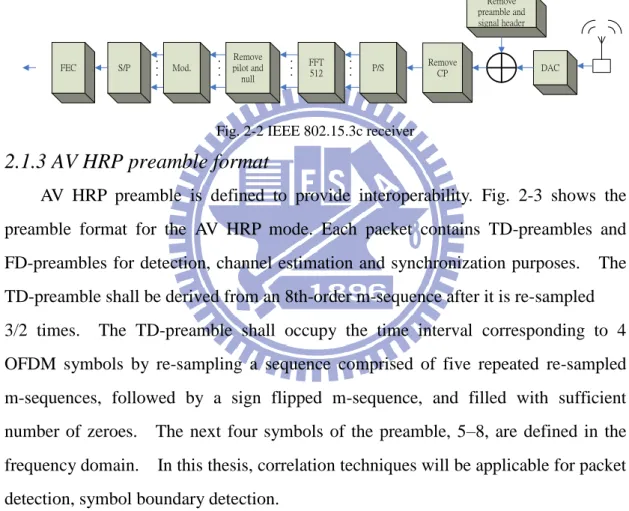
The receiver block diagram is shown as Fig. 2-2. At the receiver, the signal passes through VGA first which keeps the power level of signals and sampling after ADC. Sync is used for synchronization, including find when exactly the packet start and the OFDM symbol boundary. After that, FFT is used to transfer received signal from time domain to frequency domain. Then the bit streams are demodulation, de-interleaver and merge to single data stream. Finally, it is decoded by FEC which includes de-puncturing, Viterbi decoder and de-scrambler.

FEC S/P Mod. Remove pilot and null FFT 512 P/S Remove CP Remove preamble and signal header DAC

Fig. 2-2 IEEE 802.15.3c receiver

2.1.3 AV HRP preamble format

AV HRP preamble is defined to provide interoperability. Fig. 2-3 shows the preamble format for the AV HRP mode. Each packet contains TD-preambles and FD-preambles for detection, channel estimation and synchronization purposes. The TD-preamble shall be derived from an 8th-order m-sequence after it is re-sampled 3/2 times. The TD-preamble shall occupy the time interval corresponding to 4 OFDM symbols by re-sampling a sequence comprised of five repeated re-sampled m-sequences, followed by a sign flipped m-sequence, and filled with sufficient number of zeroes. The next four symbols of the preamble, 5–8, are defined in the frequency domain. In this thesis, correlation techniques will be applicable for packet detection, symbol boundary detection.

HRP short preamble HRP long preamble Data symbol

Short preamble#1 Short preamble#2 Short preamble#6 CP long preamble#1 long preamble#2 CP long preamble#3 long preamble#4

2304 sampling = 4 OFDM symbol

0.15μs 0.05μs 0.2μs

2304 sampling = 4 OFDM symbol

2.2 Channel model

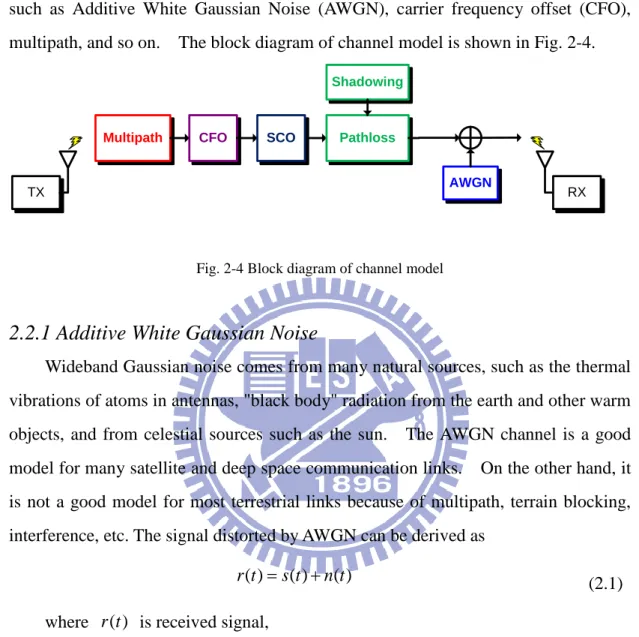
There are many imperfect effects during transmitted signals through channel, such as Additive White Gaussian Noise (AWGN), carrier frequency offset (CFO), multipath, and so on. The block diagram of channel model is shown in Fig. 2-4.

Multipath CFO AWGN RX TX SCO Pathloss Shadowing

Fig. 2-4 Block diagram of channel model

2.2.1 Additive White Gaussian Noise

Wideband Gaussian noise comes from many natural sources, such as the thermal vibrations of atoms in antennas, "black body" radiation from the earth and other warm objects, and from celestial sources such as the sun. The AWGN channel is a good model for many satellite and deep space communication links. On the other hand, it is not a good model for most terrestrial links because of multipath, terrain blocking, interference, etc. The signal distorted by AWGN can be derived as

( ) ( ) ( )

r t s t n t _(2.1)

where r t is received signal, ( ) ( )

s t is transmitted signal,

( )

n t is AWGN.

2.2.2 Multipath

In wireless communication transmission system, transmitted signal arrives at receiver through several paths with different time delay and power decay, due to there are obstacles and reflectors in the wireless propagation channel, the transmitted signal arrivals at the receiver from various directions over a multiplicity of paths. Such a

phenomenon called multipath interference. The received y n signals can be ( )

0

( )

( ) (

)

k

y n

x k h n

k

 







(2.2)

Where x(n) is transmitted signal and h(n) is channel impulse response.

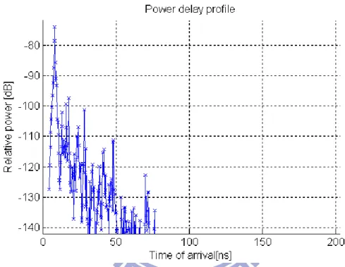
In this work, we adopt the IEEE802.15.3c CM2 channel model as reference [10]. And it average RMS delay is 3.701(ns) and average number of taps are 32.1 which the

taps power is bigger than -46dB. The power-delay profile is shown inFig. 2-5.

Fig. 2-1 IEEE802.15.3c CM2 power delay profile

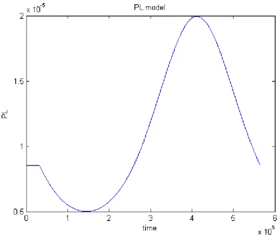
2.2.3 Path loss and dynamic shadowing

The path loss(PL) is defined as the ratio of the received signal power to the transmit signal power and it is very important for link budget analysis. Unlike narrowband system, the PL for a wideband system such as ultra-wideband (UWB) [11]-[13] or millimeter wave systems, is both distance and frequency dependent. In order to simplify the models, it is assumed that the frequency dependence PL is negligible and only distance dependence PL is modeled. The PL as a function of distance is given by

PL t d( , )PL d0( )X t( ) (2.3)

( )

X t is the dynamic shadowing fading which vibrate between -3dB to 3dB with

time variation. The vibrate period is 2π within whole packet. Assume that the transmitted signal is ( )s t and the received signal is ( )r t , then path loss effect can be

modeled as

r t

( )



s t

( )



PL t d

( , )

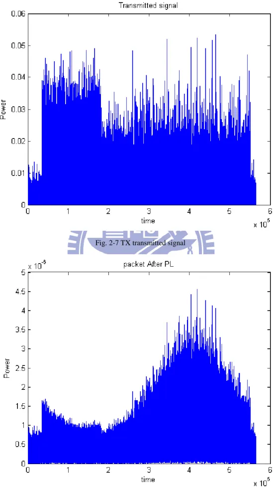
(2.4) The signals distorted by the path loss and dynamic shadowing effects is shown as Fig. 2-6 , Fig. 2-7 and Fig.2-8.

Fig. 2-7 TX transmitted signal

Chapter 3

Proposed Algorithm

In the standard of IEEE 802.15.3c, each OFDM packet has short preambles and long preambles which that they can be used to estimate the signal arrival or not, or recognize what the arrival of transmitter signal is. The received symbols are used to propose method which calculates the correlation and symbol power determines the suitable gain, packet come or not and symbol boundary decision.

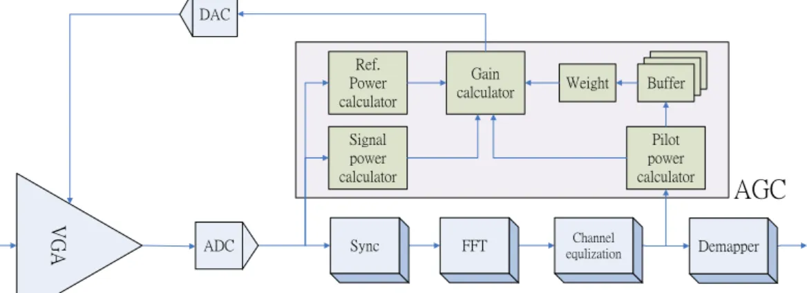
3.1 AGC

The demand of an AGC loop in wireless systems comes from the fact that all communication systems have an unpredictable receiver power. That is to say, too much gain in the receiving front-end will saturate the ADC (Analog-to-Digital Converter) and clip the signal but insufficient gain will result in higher quantization noise. Hence AGC at the receiver has much relation with ADC and reference power

in AGC is very important parameter. Fig. 3-1-1 shows the functional structure of

propose AGC scheme. VGA (Variable Gain Amplifier) is a linear-in-dB gain control circuitry. ADC is an analog-to-digital converter. Power calculator blocks calculate the average power during 48 samples of preamble or 16 samples of pilot. Ref. power calculator block calculates the rest range of ADC such that the ADC would get full swing. Weight block calculate the previous gain error cause by dynamic shadowing effects.

V G A Signal power calculator Ref. Power calculator Gain calculator Pilot power calculator Buffer Buffer Buffer Weight

Sync FFT _equlizationChannel Demapper

AGC

ADC DAC

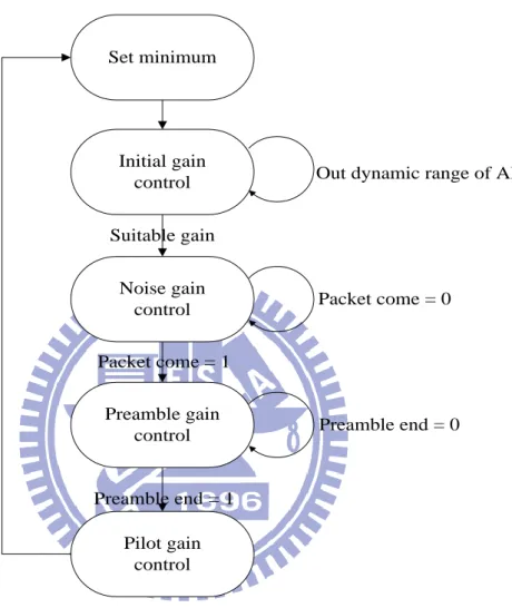
The state transition diagram implemented physically for the AGC is shown in Fig.

3-1-2. There are several control schemes in different level of packet and each state

will introduce as below.

Initial gain

control Out dynamic range of ADC

Packet come = 0 Preamble end = 0 Suitable gain Packet come = 1 Preamble end = 1 Set minimum Preamble gain control Pilot gain control Noise gain control

Fig. 3-1-2 AGC flow chart

3.1.1 Initial gain control

Initially, the received signal power must be adjusted at a suitable level, because the received signal could not be over the detecting range of ADC, the real packet information will be truncated by ADC and cause the saturation that correlator could not clearly produce correct result. For quickly justifying the VGA gain, the samplings power is used by AGC to do a large scale adjustment in VGA linear range. The concept of adjust algorithm in initial gain control is binary search, which bounds is between minimum and maximum of VGA linear range. Search until signal power

is in ADC detection range then change state to noise gain control level or preamble gain control level depends on whether packet comes or not.

3.1.2 Noise gain control

After signals power is in ADC dynamic range, the correct VGA gain that we want can directly calculate by current samplings power and ref. power we predefined. The ADC samplings power is used by AGC and the formula is

10 10 log ( ) ref N G G P    (3.1.1) Where G and G’ are current VGA gain and next VGA gain respectively. S is sampling power and D is desire sampling power defined as the signal power value with ADC five percents swing. We adjust VGA gain to keep the received signals at five percent swing of ADC to achieve low power and avoid saturation.

3.1.3 Preamble gain control

Ones the packet is coming the concept of adjustment is the same as noise level but we want to reduce the quantization noise so we must let the ADC get fully swing as possible as we can. In this state the desire VGA gain can be calculated by current signal power and ref. signal power. And the formula can be express as

10 10 log ( ) VGA VGA ref P G G P    (3.1.2)

Where G_VGA and G_VGA are current VGA gain and next VGA gain respectively. P is

current signal power and P_ref is desire signal power which is update each block

period and the initial value of P_ref is defined as the signal power with ADC fifty percents swing.

Due to the channel or some non-ideal front-end effects, P is update by ref

(quadrature-phase) components to avoid the biggest components out of ADC range. The current signal is update the reference signal power at next adjusted period such that ADC would be fully swing without saturation. The formula of the update of reference signal power is

ref ref real r t P P abs S imag r t             ( ( )) * max / ( ( )) (3.1.3) Where Pref and P is next reference signal power and current reference signal ref power respectively, and S is the sampling value with eighty percent swing of ADC.

3.1.4 Pilot gain control

Basically here is used average power of pilot to adjust VGA gain , however, owing to the size of FFT is 512 point, we regard the size of adjustment period as symbol period, that is VGA gain control period is equal to FFT period. But it’s hard to use the gain error obtained by previous symbol to adjust next symbol gain under dynamic shadowing effects. In order to adjust gain more precise, adaptive weight is used. Initially, we calculate the gain error from first two symbol and the formula of gain error calculation defined as

10

10log ( / )

t t ref

E  P P _(3.1.4)

Where Pt and Pref is mean power of pilot from current data symbol and desire

average power of pilot respectively. And the next symbol VGA gain is calculate by

1

t t t

G G  W E _(3.1.5)

Where G_t and G_t₁ are current VGA gain and next VGA gain respectively. And

the weight W is calculate by previous two gain difference E_t andE_t₁, the formula

can express as 1 1 (1 t ) t t t t E G G E E      (3.1.6)

Although we adjust VGA gain by using adaptive weight to get more precise, the performance is still loss if the dynamic shadowing effect is too worse.

3.1.5 Packet detector

The OFDM Short preambles have been designed to help the detection of the start of the packet. These preambles will enable the receiver to utilize a very simple and efficient algorithm to detect the packet. The general approach was presented in Schimdl and Cox [5] using the special preamble composed of two identical symbols to synchronize the timing. But it needs two consecutive identical preambles in their detection algorithm and the short preamble is too long in 802.15.3c that will cost too many samples to do the same things, so the cross-correlation based algorithm is used. Considering the sampling rate is fast, so the parallel cross correlation with block of sampling shift is used instead of conventional cross correlation with sampling shift.

The OFDM short training symbol r(t) are used for the packet detector. The parallel cross-correlation Pattern is defined by

1 2 3 2 1 ( ) (1) (2) (3) ( 2) ( 1) ( ) ( ) ( ) (1) (2) ( 3) ( 2) ( 1) ( ) ( 1) ( ) (1) ( 4) ( 3) ( 2) ( ) ( ) ( ) ( ) L L L Q k P P P P B P B P B Q k P N P P P B P B P B Q k P N P N P P B P B P B Q k Q k Q k Q k         _{  }                               (4) (5) (6) ( 1) ( 2) ( 3) (3) (4) (5) ( ) ( 1) ( 2) (2) (3) (4) ( 1) ( ) ( 1) P P P P B P B P B P P P P B P B P B P P P P B P B P B                    _{  }         _{ }    _(3.1.7)

And the parallel cross correlation function d(t,w) is

 

L





 

w w k d t r t k Q k   



 2 1 * 0 _(3.1.8)

Where r t



k



is the received signal, P k w



,



is the ideal pattern, dw

 

t is the cross correlation power between received signal and STF of transmitter and L is the length of sampling used in packet detection.

And the conventional decision algorithm is defined as below.

 

max(d_w t ) /S TH₁ => packet present.

 

max(d_w t ) /S TH₁ => noise present.

Where TH₁ is the threshold which we pre-define and S is signal power, if the

peak power of parallel cross correlation power over signal power is bigger than the

threshold TH₁, we determine the packet is coming, or the received signal is still

noise.

Unfortunately, there are some problem is that the AGC will not keep the full swing of ADC before packet comes. AGC will fix the noise power at 5% swing to achieve low power and avoid saturation when signal comes suddenly. But we couldn’t predict signal power via noise and we still need to wait the result of packet detector even if the signal already comes. The worse case is that the signal occupies low swing of ADC so the quantization noise increased.

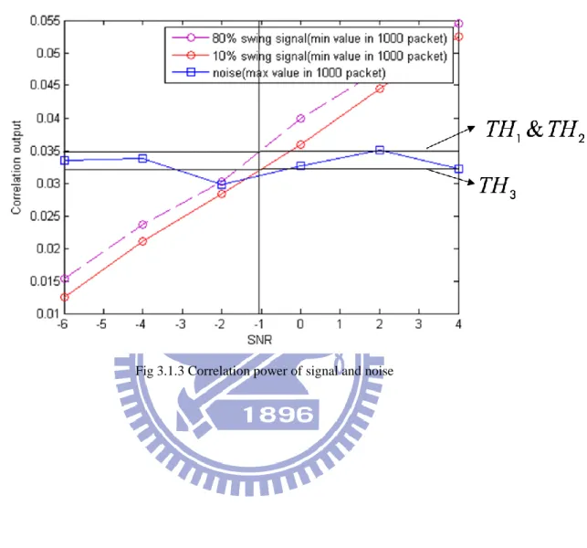
To solve the problem mentioned above, we take two thresholds TH₂ and TH₃

in packet detector. If we want there is no false alarm occurs, the threshold setting is shown as Fig. 3-1-3 which is simulation on 6 bit ADC and 48 sampling length

cross-correlation windows. TH2 is the same as TH1, and TH3 is quite lower than

TH₁. And the decision algorithm is

Case1:max(dw

 

t ) /Sn TH2 => packet present.

Case2:max(dw

 

t ) /S TH2 & max(dw

 

t ) /S TH3 => AGC adjust to high swing

regardless of signal or noise presence.

Case3:max(d_w

 

t ) /S_n TH₃ => noise present.

to high swing regardless of signal or noise when case2 occurs. Then the next block of signals after AGC adjustment is not satisfy case1, the AGC will return to noise level again circularly until packet present.

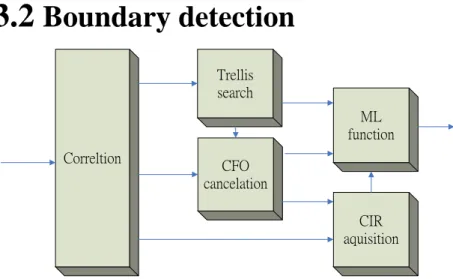
3.2

Boundary detection

Correltion _CFO cancelation Trellis search CIR aquisition ML function

Fig. 3.2.1 Block diagram of boundary detection

The proposed algorithm has 3 steps to estimate symbol boundary of receive signal: 1. Use cross correlation to determine symbol boundary depend on correlation output. 2. Sequential search the symbol boundary by three correlation outputs during three blocks of sampling shift.

3. CIR(channel impulse response) acquisition by correlation output and ML(maximum likelihood) function is used to determine the final symbol boundary with CFO cancelation.

3.2.1 Parallel cross correlation

Correlation is a mathematical tool used in signal processing for analyzing functions or series of values, such as time domain signals. Correlation is one of the most common and the most useful statistics. To detect the symbol boundary correctly, the cross-correlation is the correlation of two different signals to determine symbol boundary currently. But the TD-preamble is been re-sample at transmitter in 802.15.3c so it wouldn’t get good correlation property if we use conventional cross correlation pattern. Here, we propose a new parallel cross correlation metric which has better correlation property. At the receiver, the received signal of TD training symbol becomes

2

( )

( ( )

( ))

j πf kTs

( )

r t



h t



s t



e





N t

17

Where N is the complex AWGN, ( ) [ , ,_{0 1} , ]

m

T L

h t  h h h is a vector containing

Ts-spaced samples of the channel response, s t( ) is the tth element in training

sequence. We will separate the receive signals ( )r t to three segments, R1, R2 and

R3 _{.Which is defined as below}

s1 s2 s3 s4 s5 s6 ... s94 s95 s96 s1 s4 s7 ... s94 s2 s5 s8 ... s95 s3 s6 s9 ... s96 Separator correlation buffer Received signals C o rr el at io n b u ff er R1 R2 R3

Fig. 3.2.2 Signal separator 1 0 ( 3 ) B L k R r t k L       (3.2.2) We first defined the parallel cross correlation pattern

2 3 L_B matrix as 1 3 5 4 2 ( ) (1) (3) (5) ( 4) ( 2) ( ) ( ) ( ) (1) (3) ( 6) ( 4) ( 2) ( ) ( 2) ( ) (1) ( 8) ( 6) ( 4) ( ) ( ) ( ) ( ) L L L Q k P P P P B P B P B Q k P N P P P B P B P B Q k P N P N P P B P B P B Q k Q k Q k Q k         _{  }               _{ }             (7) (9) (11) ( 2) ( 4) ( 6) (5) (7) (9) ( ) ( 2) ( 4) (3) (5) (7) ( 2) ( ) ( 2) P P P P B P B P B P P P P B P B P B P P P P B P B P B                    _{  }         _{ }    _(3.2.3)

Where P is the ideal training sequence before it is re-sampled, L is the length

of training sequence and B is the length of correlation window.

And the parallel cross correlation function is





 

2 1 * , 0 B L w L w k d R t k Q k   



 (3.2.4) Separate buffer R(#1~#3) Cross correlation . . . . 1 Q 2 Q 3 Q L Q Known training sequence

Fig. 3.2.3 Parallel correlator

The concept of this correlation metric is avoid to use the sampling which is been

re-sample at transmitter. So we would estimate symbol boundary index by dL w,

and the formula is

, , ˆ _{arg max{ }} index L w L w Symbol  d (3.2.5)

3.2.2 Trellis search

But it’s not precise enough if we only do parallel cross correlation one time under channel effects. So we do the parallel cross correlation for K times and defined a search rule to estimate symbol boundary. Then we check the solution by collecting the K sets of parallel cross correlation value during K block of sampling

period. We denote each index of correlation pattern refer to a sample index as di j k, , .

Where i is one of three segment of signals separation, j is the index of correlation patterns and k is one of kth block of sampling shift. And we only consider Z correlation outputs which the correlation power is bigger than the other correlation outputs in each correlation block. And the di j k, ,  dl m n, , is allowable state transition

if j i   B m l and n k 1 _{just like Fig. 3.2.4. With applying the allowable}

as   ( , , ) , , 1 k j di j dl m K



    _{ } (2.5) i=1 j=3 i=2 j=98 i=1 j=42 i=3 j=5 i=1 j=30 i=3 j=140 i=1 J=99 i=3 j=195 i=3 j=234 i=3 j=197 i=2 j=222 i=2 j=310 max min K1 K2 K3 Survival path

Fig. 3.2.4 Trellis diagram

And the each different survivor paths are our candidates of the symbol index. We determine the final result by the summation of correlation power with three blocks correlation results. And which symbol index contains the maximum correlation value is the best option in the set of

 

k_j

3.2.3 Maximum likelihood

Although we used parallel cross correlation and trellis search to find the best option of symbol boundary. But the performance isn’t good enough, due to bad correlation property in re-sampled training sequence. So we propose a method based on ML after trellis search. First, we found the CIR corresponds to each pattern from parallel cross correlation result. And the formula could be express as

* , * , , L k nk k n L n k n k k r p T p p     





1 0 1 0 _(3.16)

But it is sensitive under CFO effects, so we must do CFO cancelation first to avoid CFO effects. We already have correlation output of each pattern from previous parallel correlation so we choose the pattern index j which has maximum correlation power in trellis survival path. Then we could divide the correlation between each block of sampling shift cross-correlation output. And the formula is shown as below: ( ) * * , , ( ) * * , , s s s L L j f D k T D k D n k D k D n k j f D k T j f kT k k L L j f kT k n k k n k k k r e p r p z e r e p r p                        











1 1 2 2 2 0 0 1 1 2 0 0 (3.17)

Then we could get the CFO information by the angle difference from z.

1 1 ( ) tan ( ) 2 _s ( ) image z f πDT real z     (3.18) Fig 3.2.5 shows the Mean absolute error of CFO estimation. This CFO estimator may be not precise than general CFO estimator which used repeated symbol structure due to it suffer from inter symbol interference caused by multipath fading. But it is precise enough to do the CIR acquisition and maximum likelihood function.

After we get the CFO information by previous estimation method, the CIR acquisition by cross-correlation could consider the rotation caused by CFO to get more accuracy. The formula of CIR acquisition would become

* , * , s , L k nk k n _L j f kT n k n k k r p T p e  p     





 1 0 1 2 0 _(3.19)

Although the taps correspond to each pattern is known but the absolute position of each taps in CIR is unknown. Only relative position of each taps is obtained by pattern index order and it shown as Fig. 3.2.6. In order to recovery the original signal to make maximum likelihood function correctly, we must find the initial tap in CIR. So we defined matrix H by the channel taps with circular shift that we get from correlation and matrix P which is the pattern sequence corresponds to the each channel taps.

{ , , , } { , , , } { , , , } k k k n k k k n n k n k n k h T T T h h T T T h h T T T h                 _       _{ }      _        1 1 1 1 2 1 2 2 1 2 3 Η 1 2 1 1 2 3 2 3 4 1 1 1 2 n n n n n n n n n n n n n p p p p p p p p p p p p p p p p                            P (3.20) And another ML function which is used to find the correct CIR is defined as below

Δ 2 , 0 arg min( ( ) s ) L j πf kT k ii k i _k r e  



 c h ΗP (3.21) When the correct CIR is determined, we could check the symbol boundary candidate which is produce by previous trellis result. We defined a mask matrix corresponds to each symbol boundary candidate and a ML function to get the final decision about symbol boundary. Δ 1 2 0 arg max( ( ) s ) L j πf kT k t t k m r e n trellis candidate   



 M h Pc n k  (3.22) Where M is a mask matrix correspond to each trellis candidate that we want to make

decision from them. So the symbol boundary t corresponds to minimum value m

in trellis candidate is the best option of the symbol boundary. But it is obviously that the complexity of those matrix computations in ML function is high, so we must reduce it complexity without performance loss in symbol boundary decision. Fortunately, the second ML function could be reduce as follow

Δ Δ

1 1

2 2

,

0 0

arg min( ( ) s ) arg max( (( ) ) s )

L L j πf kT j πf kT k t n k k t t _k t _k r T p e r e       





M hc Pn k (3.23) The right term of equal symbol is mask the taps correspond to trellis candidate then find the maximum value produce by ML result and the left term of equal symbol is only consider the taps correspond to trellis candidate then find the minimum value from ML. Under this formula derivation, the first ML which is used to find correct position of each taps in CIR is unnecessary because we only need to know which taps correspond to the which pattern index. As mentioned above, we could get some

complexity reduction to make this method more feasible. Table 3-1 shows the complexity derivation as mentioned above. Original ML means the original concept to do boundary detection and we could reduce the complexity by equation 3.23 and finally combine trellis result to reduce the region of detection.

Original ML ML reduction Combine

coarse detect Parallel cross correlation 32*128*3(multiplication) 31*128*3(addition) CIR acquisition 383 (division) 383 (division) 6 (division) Initial taps acquisition 383*383*288 (multiplication) 382*288 (addition) 0 0 ML function 383*382*288 (multiplication) 383*288 (addition) 383*288 (multiplication) 383*288 (addition) 6*288 (multiplication) 6*288 (addition)

Chapter 4

Simulation

The simulation results for AGC, packet detection and boundary detection algorithms are shown in this chapter. MATLAB is chosen as simulation language, due to its ability to mathematics, such as matrix operation, numerous math functions, and easily drawing figures. And the parameters are shown in Table 4-1.

Parameter Value Modulation 16 QAM

Coding Rate 2/3

PSDU Length 1024 Bytes

Packet No 2000

FFT size 512

width and depth of ADC 6 and 8

Path Loss -20dB to -80dB

Shadowing vibrate 3dB

Channel Model IEEE802.15.3c CM2

RMS delay spread 4 ns

CFO 40ppm

SCO 40ppm

Equalization Zero-Forcing

Table 4-1 Simulation parameter

4.1 AGC

Fig. 4-1 and Fig. 4-2 are the signal of VGA inputs and the signal of ADC outputs respectively. The signal is suffer from path loss and dynamic shadowing effects so the input signal will be very small and vibrates in time. After AGC control we could see that the signal of ADC outputs is more stable and keep in the dynamic range of ADC. At the noise level, AGC would let VGA achieve low power and avoid signal saturation when signal comes suddenly. At the signal level, AGC would track the rest range of VGA to get stable without saturation by 96 samplings.

Fig. 4-1 VGA input signal

Fig. 4-2 ADC output signal

Fig. 4-3 shows that the propose AGC adjustment result compare with desire VGA gain when shadowing period 2π within whole packets when SNR is 10dB. AGC would track the shadowing effects such that the adjustment of VGA to form a sine wave. Although there are a little gain errors caused by AWGN effects but it still in acceptable region.

Fig. 4-3 Adjustment of VGA

Fig. 4-4 shows the performance of the proposed packet detection algorithm.

It’s Simulation in 48 sampling length as correlation windows. TH₂ and TH₃

is set 0.035 and 0.0325 as Fig. 3.1.3. We evaluate the performance of the

algorithms by plotting the packet detect error rate against the SNR. Packet

detection error rate means the number of packet detection error over the number of transmitted packets and misdetection means we detected the packet over 96 sampling of each packet when packet comes. Packet detection error includes false alarm and misdetection. On the Fig. 4-4, this approach would lower the quantization error to improve the performance of packet detection.

Next we compare the performance between propose AGC and conventional AGC algorithm [1][2] which is constant reference power and without adaptive weight on the Fig. 4-5. When dynamic shadowing effects is 2π, the propose AGC is 0.8dB loss in SNR compare with ideal AGC at PER 1% and the conventional AGC is 2.6dB loss in SNR compare with ideal AGC. The propose AGC gain 1.8dB in SNR under dynamic shadowing effects. Regardless of propose AGC or conventional AGC the performance will get worse when dynamic shadowing effects become worse. But the resistance of dynamic shadowing effects is more obviously between them. There is 3.5dB loss of SNR at PER 1% between propose AGC and conventional AGC under dynamic shadowing effects is 2.5π.

Fig. 4-5 PER of AGC for different level of shadowing effects

4.2 Boundary detection

The settings of the proposed boundary detection are B=96, Z=6, K=3. We evaluate the performance of the algorithms by plotting the Boundary error rate against the SNR. The Boundary error is defined by sample offset is over two or more samples. The correct symbol boundary of OFDM symbols can be tolerant of ±1 sample offsets. Fig. 4-6 shows the performance of the proposed algorithm and conventional cross correlation metric reference as [7][8]. And Fig. 4-7 shows the estimated position with

respect to ideal position at SNR=5.

Fig. 4-6 Boundary error rate of different detect method

The conventional correlation metric isn’t work in this platform due to bad correlation property. And the propose correlation metric would improve the performance but isn’t good enough and we could get much better performance to achieve less than 0.1% at SNR=6. Fig. 4-8 shows the boundary error rate in the CFO range of ±400 ppm. The results indicate that the synchronization performances degrade insignificantly if CFO is less than ±200 ppm. The high CFO resistance also means the proposed synchronizer being well-suited to most wireless standards without pre-compensation of frequency errors

Chapter 5

Conclusion and Future Work

5.1 Conclusion

In this thesis, we introduce automatic gain control and frame synchronization algorithm for 802.15.3c systems. The path loss and dynamic shadowing effects could be solved by AGC with several schemes to prevent saturation or suffer high quantization noise from ADC and get only 0.8dB loss compare with ideal case. And the propose frame synchronizer could work well on 802.15.3c system by combine cross-correlation and ML method.

5.2 Future work

The performance of AGC still get relative loss of SNR under dynamic shadowing effects get worse, so it must need more complex calculation to approach the behavior of shadowing effects.

The trend of wireless broadband communications had created the need of frequency-domain front-end receivers that can relax the analog-to-digital requirements and benefit the suppression of narrow band interference. The concepts of this work would try to translate from time domain to frequency domain.

Bibliography

[1] V.P.G. Jimenez , M.J.F.-G. Garcia , F.J.G. Serrano and A.G. Armada, “Design and implementation of synchronization and AGC for OFDM-based WLAN receivers”,

IEEE Trans. Consum. Electron, vol. 50, no 4, pp 1016–1025, Nov 2004.

[2] A. Fort , W. Eberle, “Synchronization and AGC proposal for IEEE 802.11a burst OFDM systems” Global Telecommunications Conference, 2003. GLOBECOM '03.

IEEE, pp 1335–1338, Dec 2003 .

[3] J. V. D. Beek, M. Sandell, and P. O. Borjesson, “ML estimation of timing and frequency offset in OFDM Systems” IEEE Tran.on Signal Processing, vol. 45, no 7, pp. 1800-1805, July 1997.

[4] K.Wang, M.Faulkner, J. Singh and I.Tolochko, “Timing synchronization for 802.11a WLANs under multipath channels” ATNAC, Melbourne, Dec 2003

[5] T. M. Schmidl and D. C. Cox,“ Robust Frequency and Timing Synchronization for OFDM” IEEE Trans. on Communications, vol. 45, no. 12, pp. 1613-1621, Dec. 1997. [6] S. H. Muller-Weinfurtner, “On The Optimality of Metrics for Coarse Frame Synchronization in OFDM: A Comparison” PIMRC 98, pp533- 537, Sept. 1998, Boston, MA.

[7] F. Tufvesson, O. Edfors, and M. Faulkner, “Time and frequency synchronization for OFDM using PN-sequence preambles” in Proc. Vehicular Technology Conf. (VTC),

Amsterdam, The Netherlands, 1999, vol. 4, pp 2203–2207.

[8] B. Yang, K. B. Letaief, R. S. Cheng, and Z. Cao, “Timing recovery for OFDM transmission” IEEE J. Sel. Areas Commun., vol. 18, no. 11, pp. 2278–2291, Nov. 2000.

[9] S Nandula, K Giridhar, “Robust timing synchronization for OFDM based wireless LAN System,” Proc. IEEE International Conference on Convergent Technologies for

Asia-Pacific Region, TENCON 2003, vol 4C, pp. 1558-1561, Bangalore, India, 2003.

[10] S. Yong, “TG3c Channel Modeling Sub-committee Final Report”, Samsung

Advanced Institute of Technology, March 2007.

[11] A. Mathew and Z. Lai, “Observations of the UMass Measurements,” IEEE

802.15.06-0137-00-003c, Denver, Mar 2006.

[12] A. F. Molisch, D. Cassioli, C. –C. Chong, S. Emami, A. Fort, B. Kannan, J. Karedal, J. Kunisch, H. Schantz, K. Siwiak, and M. Z. Win, “A comprehensive standardized model for ultrawideband propagation channels,” IEEE Trans. Antennas

[13] C. -C. Chong Y. E. Kim, S. K. Yong and S. S. Lee., “Statistical characterization of the UWB propagation channel in indoor residential environment,” Wiley J. Wireless

Commun. Mobile Comput. (Special Issue on UWB Communications), vol. 5 no. 5, pp.

503-512, Aug. 2005.

[12] J. Lago-Fernández. and. J. Salter J. Lago-Fernandez and J. Salter, “Modelling impulsive interference in DVB-T: statistical analysis, test waveforms & receiver performance”, R&D white Paper, WHP080, April 2004.

[13] M.C. Jeruchim, P. Balaban, K.S. Shanmugan, Simulation of Communication

Systems: Modelling, Methodology, and Techniques, 2nd Ed., Kluwer Academic / Plenum Publishers, Aug 2000.

[14] K. L. Blackard, T.S. Rappaport, and C.W. Bostian, “Measurements and Models of Radio Frequency Impulsive Noise for Indoor Wireless Communications”, IEEE

Journal on Selected Areas in Comms., Vol. 11, No. 7, Sep 1993.

[15] Yahya, Mazlaini,” Practical Packet Detection and Symbol Timing Synchronization Scheme for Packet OFDM System” RF and Microwave Conference,

2006. RFM 2006. International, pp. 421 – 425, 12-14 Sep. 2006

[16] T. Liang, X. Li, R. Irmer, G. Fettweis, “Synchronization in OFDM-based WLAN with transmit and receive diversities” Personal, Indoor and Mobile Radio

Communications, 2005. PIMRC 2005. IEEE 16th International Symposium on, Vol.

2, pp. 740-744, Sep 2005

[17] B. Kim ; C. Shin ; S. Choi; “Packet detection scheme using cross correlation and

complex multiplication in MB-OFDM UWB system”Information, Communications