成像與非成像光學系統之光學傳遞函數分析與應用

(1)

國立交通大學

光電工程研究所

博士論文

成像與非成像光學系統

之光學傳遞函數分析與應用

Optical transfer function and its

applications to imaging and

non-imaging optical systems

研究生 : 鄭竹明

指導教授 : 陳志隆教授

(2)

成像與非成像光學系統

之光學傳遞函數分析與應用

Optical transfer function and its applications to

imaging and non-imaging optical systems

研究生：鄭竹明 Student：Chu-Ming Cheng

指導教授：陳志隆 Advisor：Jyh-Long Chern

國立交通大學

光電工程研究所

博士論文

A Dissertation

Submitted to Institute of Electro-Optical Engineering College of Electrical and Computer Engineering

National Chiao Tung University in partial Fulfillment of the Requirements

for the Degree of Doctor of Philosophy

in

Electro-Optical Engineering May 2010

Hsinchu, Taiwan, Republic of China

(3)

成像與非成像光學系統之

光學傳遞函數分析與應用

博士研究生 : 鄭竹明指導教授 : 陳志隆教授

國立交通大學光電工程研究所

摘

要

對於當今的光學儀器與光電消費性產品而言，除了被要求微型化系統設計之外，追求更優質的影像品質和高光學效率以及細緻的解析度畫質亦是未來光電產品的重要趨勢與主流。在成像光學系統的領域中，全幅對焦技術(EDOF,

extending the depth of focus) 已然成為一個非常重要的光學設計議題。本論文利用光學傳遞函數 (OTF, optical transfer function) 和照明分布函數，開發出一套解析和半解析式數學模型，並將此方法應用於非同調成像光學系統之成像與非成像光學品質的評估與分析。由於照明光場會改變待測物的反射光強度分佈，因此我們不能再假設一成像系統中，待測物的光學傳遞函數值為一。所以，我們利用光闌方程式 (pupil function) 中的振幅穿透方程式 (一個描述非成像光學特性的項) 和波像差方程式(一個描述成像光學特性的項)，深入地探討光學傳遞函數和照明光分布之間的相互關係。本論文的學術貢獻之ㄧ，是在一光學系統的光學傳遞函數計算中，加入一”非成像光學”的有效因子，進而能夠完整地分析與評估光學系統的成像品質。我們也進一步地提出一種新的全幅對焦光學技術，並驗證於非同調成像光學系統之中。此技術利用在非成像系統中，設計一個空間光學調變器來產生一個結構光束(structured light)，如數位微鏡片元件(DMD, digital micromirror device)或是發光二極體陣列裝置(LED array module)，以提供一動態可程式化變形光闌 (a dynamically programmable shaped pupil)，並將此變形光闌投影在成像光學系統的孔徑位置。我們使用自行開發的光學傳遞函數之半解析式數學模型，驗證此新技術可以有效地補償光學像差，如失焦、球差和彗差等，同時亦可提升光

(4)

學系統的成像解析力。我們的研究是連結和整合成像與非成像光學系統的特性，開發出一新全幅對焦光學技術，應用一嵌入式照明調變器，達到提升傳統非同調光學系統的成像光學品質以及擴展其光學系統的對焦深度，並將此技術應用於光導管、攝影機、顯微鏡和投影機等光學系統中。

(5)

Optical transfer function and its

applications to imaging and

non-imaging optical systems

Doctoral Student：Chu-Ming Cheng Advisor：Dr. Jyh-Long Chern

Institute of Electro-Optical Engineering

National Chiao Tung University

Abstract

Today’s optical instruments and electro-optical consumer products demand high imaging quality, optical efficiency and high resolution with the volume of the machine, nevertheless, being compact. At the same time, extending the depth of focus (EDOF) in an imaging system has been a long-standing issue in optical designs. This thesis develop either an analytical or a semi-analytical model by the use of optical transfer function (OTF) and illumination formations on the study of imaging and non-imaging qualities in the incoherent imaging system. Since the illumination light could vary the intensity distribution of the reflective light from an object, we could no longer assume the OTF of the object equal to unity in an imaging system. Hence, we make the in-depth investigation into the relationship between OTF and the illumination light distribution by calculating the OTF using the pupil function with the amplitude transmittance function which is the term given to the characteristic of a non-imaging system, and the wave aberration function which is the term given to the characteristic of an imaging system. One of main contributions of this thesis is to implement and demonstrate the effective factor of the non-imaging system (i.e., illumination light) in OTF calculation for assessing and specifying the performance of an imaging system. Then, a new approach for EDOF in an incoherent imaging system has been demonstrated. It provides a programmable shaped pupil using structured light which is generated by a non-imaging system with a spatial light modulator such as the digital micromirror device (DMD) or the light-emitting-diode (LED)-array module. The semi-analytical results using the OTF indicate that the limiting resolution of an

(6)

imaging system with a specific defocus coefficient, and the specific coefficients for spherical aberration and coma aberration can be improved significantly with a binary shaped pupil. The proposed structured light on aperture stop from the non-imaging system can offer a dynamically programmable approach for aberration compensation in an incoherent imaging system. Our proposed research provides the connection between non-imaging and imaging systems for extending the depth of focus and further enhancing the image quality in the conventionally incoherent imaging systems for light pipe, camera, microscope and projector with embedded illumination modulator.

(7)

誌謝

投入光電產品的研發和光學工程的研究已有12 多年的時間，自己很榮幸擁有這麼好的因緣際會，能夠在光電科學領域中，持續地從事技術的創新和學術的研究。首先，非常感謝交通大學光電工程研究所，能夠提供這麼優質地學習與研究的環境，以及特別地感謝指導教授陳志隆教授多年來的指導，其淵博的學識和嚴謹的研究精神，給予學生許多的教導與啟發。同時，感謝博士論文口試委員黃中垚教授、蘇德欽教授、趙于飛教授、施宙聰教授以及何明宗教授，提供學生許多寶貴的意見；亦感謝鄭伊凱同學、鄭介任同學和曹兆璽同學平時的幫忙與鼓勵。此外，感謝揚明光學股份有限公司，提供學生在職進修的機會，以及由衷地感謝徐誌鴻總經理長期以來對後輩的提攜與教導；亦感謝林宗彥副總、邱賢琪副總、謝啟堂協理、鍾博任協理、張維勝協理、廖洽成協理、劉永光協理和康尹豪資深研究員等老長官們，長年來對我的勉勵與指導；同時，我更要特別地謝謝親密的工作夥伴林維賜、陳時偉、陳皇銘、蔡志賢、范萬昌、林清民、張美雲、李育宗、許志祿、陳錦怡、吳怡慧、陳孟萱、楊勝捷、黃習能和其他許多同事們相互的激勵，使得這麼多年來的工作充滿了衝勁與喜悅。最後，謹將此論文獻給最親愛的父母、兄長以及最可愛的老婆和孩子們，謝謝他們平日來給予我最溫馨地關懷與支持。我會繼續努力地在光電工程領域上發明與創新，期許自己能夠為人類、科學與社會，創造出更多實質的福祉與貢獻。

(8)

Figure Captions

Figure 1-1 Comparison of imaging and non-imaging optical systems...6

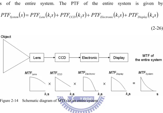
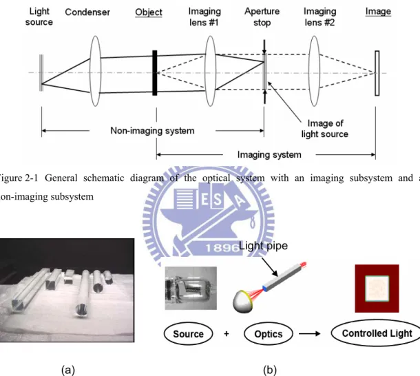
Figure 2-1 General schematic diagram of the optical system with an imaging subsystem and a non-imaging subsystem ...9

Figure 2-2 (a) The photograph of the light pipe with circle and rectangular shapes[29] and (b) the illustration of an illumination system with a light source and a light pipe for a uniform light output [30]. Illumination system provides a desired light distribution that may have little or no relationship to light distribution from the light source. Figure (b) shows an illumination system with a filament in a reflector which can provides a uniform light distribution at the end of a square light pipe...9

Figure 2-3 (a) The photograph of a DSLR camera with flash light[31], (b) cutaway of an Olympus E-30 DSLR camera [32], (c) cross-section view and introduction of a DSLR camera [32]and (d) the schematic diagram of a photographic system with a camera, an imaging system, and a flash light, a non-imaging system. ...10

Figure 2-4 (a) The photograph of a projector- Optoma EP755 model[33], (b) cross-section view and introduction of a DLP projector,and (c) the schematic diagram of a projector system with a projection lens, an imaging system, and a light pipe illumination, a non-imaging system...11

Figure 2-5 (a) The photograph of an optical microscope [34], (b) cross-section view and introduction of a microscopic illumination system [35], (c) cross-section view and introduction of the illumination light path and image-forming light path in microscope [35]. The schematic diagrams of a microscopic system with an imaging lens, an imaging system, and an illumination, a non-imaging system are for (d) a transparent sample and (e) a reflective sample. ...12

Figure 2-6 Illustration for defining the aberration function. [1]...13

Figure 2-7 Typical plot of MTF and PTF versus spatial frequency. [36]...15

Figure 2-8 Illustration of an LED light source radiating into a surface...16

Figure 2-9 Measurement locations at the center of nine equal rectangles of a 100% exit plane on irradiant surface. The four corner points 10, 11, 12 and 13 are located at 10% of the distance from the corner itself to the center of the measurement location 5[38]...17

Figure 2-10 Variation of the Ètendue with the tangential f-number, (f / #)-T, for a variety of the sagittal f-number, (f / #)-S, i.e., from 1.0 to 4.0, in the optical system. ...21 Figure 2-11 The illustration of the MTF and spatial frequency in a lens system. [42]

(12)

...24 Figure 2-12 (a) A plot of MTF against "spatial frequency" for different designs of f /4 and f /8 lens, (b) the effect of defocus on MTF for an f /2.8 lens. [43]...26 Figure 2-13 (a) An image of USAF 1951 US Air Force resolution test chart [44], (b) A record of the test chart in a film or a detector through the lens in an optical system. ...27 Figure 2-14 Schematic diagram of MTFs in an entire system...28 Figure 3-1 Schematic diagrams of the optical projection system with the light pipe

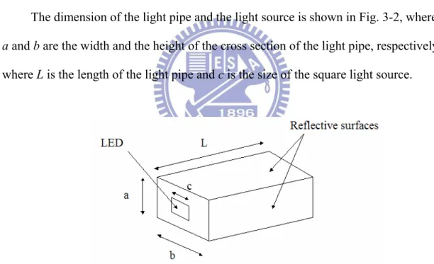
and light-valve to illustrate the relationship between pupils and fields..31 Figure 3-2 Schematic diagrams and Dimension of the light pipe and LED source. .32 Figure 3-3 (a) Principle operation of light pipe. (b) Image at the aperture stop in the

optical system. The light pipe is made with the parallel reflective sides with the rectangular cross section. The multiple reflections of the light source through the pipe can produce the spatially

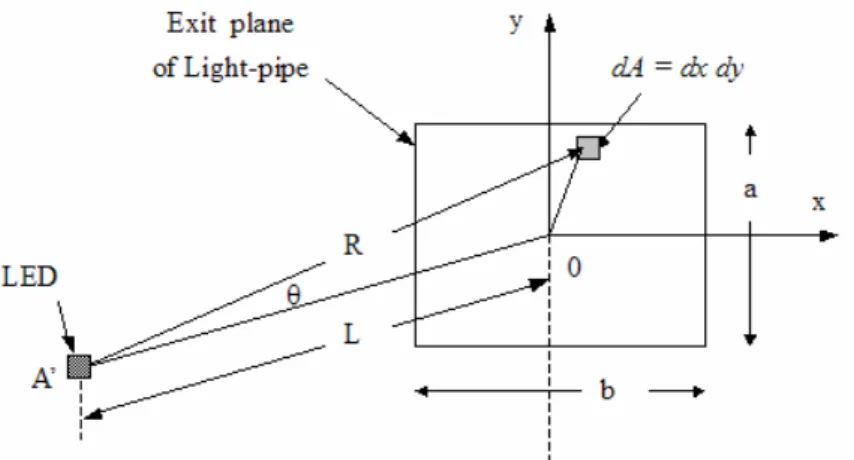
checkerboard-array-shaped light distribution, a virtual image at the entrance of the light pipe...33 Figure 3-4 LED spatial light-intensity distribution’s chart. ...34 Figure 3-5 Geometry of a LED source radiating into the exit plane of the light pipe.

...35 Figure 3-6 Illustration of a LED source radiating into the exit plane of the light pipe

for the different virtual light spot on the entrance plane of the light pipe. ...36 Figure 3-7 Total aperture functions on the normalized pupil in the condition of D=20, a=b=2.5 and L= 60 with (a) c=0.5, (b) c=1.0, (c) c=1.5, (d) c=2.0. ...40 Figure 3-8 Total aperture functions on the normalized pupil in the condition of D=20, c=2.0 and L= 60 with (a) a=b=2.5, (b) a=b=3.5, (c) a=b=5.0, (d) a=b=7.5, (e) a=b=10.0...41 Figure 3-9 Total aperture functions on the normalized pupil in the condition of D=20, a=b=2.5 and c=2.0 with (a) L=20, (b) L=30, (c) L=60, (d) L=120. ...42 Figure 3-10 Optical transfer functions in aberration-free system with a clear aperture

T0 and specific apertures generated by different light pipe’s geometric

structure with fixed a=b=2.5 and fixed L= 60 and different conditions of c=0.5, c=1.0, c=1.5 and c=2.0...45 Figure 3-11 Optical transfer functions in aberration-free system with a clear aperture

structure with fixed c=2.0 and fixed L= 60 and different conditions of a=b=2.5, a=b=3.5, a=b=5.0, a=b=7.5 and a=b=10.0. ...46 Figure 3-12 Optical transfer functions in aberration-free system with a clear aperture

(13)

structure with fixed a=b=2.5 and fixed c= 2.0 and different conditions of L=20, L=30, L=60 and L=120...47 Figure 3-13 Optical transfer functions in defocused system with (a) a clear aperture

and (b) one specific aperture generated by different light pipe’s geometric structure with a=b=2.5, c= 2.0 and L=60 for the different defocused coefficients ω20= 0, λ/π, 2λ/π, 3λ/π, 5λ/π and 10λ/π...48 Figure 4-1 Schematic diagram of the incoherent imaging system with the DMD™

and the total-internal-reflection (TIR) prism subsystem...53 Figure 4-2 Illustration of the binary amplitude transmittance T ′

( )

x,y for the

normalized circular aperture which is generated by the DMD™. T

( )

x,y represents a specifically shaped aperture for a conventional annular apodizer...55 Figure 4-3 Binary Amplitude transmittance T ′

( )

x,y with T(x, y) =1- (x2+y2) on the

normalized pupil in the condition of D=2, and scale ratios at (a) K=0, (b)

K=0.05, (c) K=0.1, and (d) K=0.3, which are generated by DMD™. ....58

Figure 4-4 Binary Amplitude transmittance T ′

( )

x,y with T(x, y) =1 on the normalized pupil in the condition of D=2 in different conditions of (a)

c=0.05, (b) c=0.1, (c) c=0.15 and (d) c=0.2, which are generated by

DMD™. ...60 Figure 4-5 Optical transfer functions in an aberration-free system and a defocused

system with different defocused coefficients (a)

ω20= 0, (b) ω20= λ/π, (c) ω20= 3λ/π, (d) ω20= 5λ/π, (e) ω20= 10λ/π and (f)

ω20= 15λ/π, for binary amplitude transmittances of the aperture functions

for K=0.05, K=0.1, and K=0.3, which are generated by the DMD™, and for a clear aperture T(x, y) = 1 and one specific shaped aperture T(x, y) =1- (x2+y2) of a conventional annular apodizer, respectively...63 Figure 4-6 The computer-simulated images of spoke patterns for A, a clear aperture,

and B, a specific shaped aperture with the scale ratio K=0.05 obtained with different defocused coefficients: (a)

ω20= 0, (b) ω20= 5λ/π, (c) ω20= 10λ/π and (d) ω20= 15λ/π. ...65

Figure 4-7 Optical transfer functions in an aberration-free system with a clear aperture and the binary amplitude transmittances of the aperture functions for different conditions of c=0.05, c=0.1, c=0.15 and c=0.2, which are generated by the DMD™...66 Figure 5-1 (a) A schematic diagram of structured lighting system for 3D Scanning

[56]. (b) From left to right: a structured light scanning system containing a pair of digital cameras and a single projector, two images of an object

(14)

illuminated by different bit planes of a gray code structured light sequence, and a reconstructed 3D point cloud[57]...70 Figure 5-2 A schematic diagram of the structured lighting system for a conventional wide-angle microscopy [55] where (a) is an autofocus image of lily pollen grain, obtained by the structured lighting microscopic system. The field size is 100µm × 70µm. (b) Conventional image of lily pollen grain when the microscope is focused in a mid-depth plane. ...71 Figure 5-3 General schematic diagram of the Köhler illumination system and the

conjugate focal planes...72 Figure 5-4 Schematic diagram of the modified Köhler illumination system with a

shaped aperture using the structured light and the conjugate focal planes. ...73 Figure 5-5 Schematic diagrams of the optical systems with one incoherent imaging

subsystem and one non-imaging subsystem to illustrate the relationship between the aperture stop and the field for (a) a reflective object and (c) a transparent object...75 Figure 5-6 Schematic diagram of the projector system with a Köhler illumination

subsystem and a projection subsystem to illustrate the relationship between the aperture stop and the digital micromirror device. The dotted and solid lines indicate the optical path of the illumination rays in a Köhler illumination system. The dashed lines indicate the optical path of the imaging rays in a projection system...77 Figure 5-7 Schematic diagrams of the optical systems in microscopy with DMD

illumination modulator for (a) a transparent sample and (b) a reflective sample. ...79 Figure 5-8 Illustration of the binary amplitude transmittance T ′

( )

x,y for the

normalized circular aperture which is generated by the DMD™. T

( )

x,y represents a specifically shaped aperture for a conventional annular apodizer...81 Figure 5-9 Total aperture functions on the aperture stop, which are generated by the

DMD™ in the conditions of (a) clear aperture, (b) K=0, (c) K= 0.05 and (d) K= 0.3. ...83 Figure 5-10 Amplitude transmittance T ′

( )

x,y with T(x, y) =1 on the normalized

pupil in the condition of D=2 and the fill factors (a) 100%, (b) 90%, (c) 80%, (d) 70%, (e) 60% and (f) 50%. ...85 Figure 5-11 Optical transfer functions in an aberration-free imaging system and a

defocused imaging system without spherical aberration ω40= 0 and coma

(15)

ω20= 0, ω20= λ/π, ω20= 3λ/π, ω20= 5λ/π, ω20= 10λ/π and ω20= 20λ/π for

amplitude transmittances of the aperture functions for (a) clear aperture, (b) K= 0, (c) K= 0.05, and (d) K= 0.3. ...88 Figure 5-12 Optical transfer functions in an aberration-free imaging system and an

imaging system without defocus aberration ω20= 0 and coma aberration

ω31= 0, but with different spherical aberration coefficients

amplitude transmittances of the aperture functions for (a) clear aperture, (b) K= 0, (c) K= 0.05, and (d) K= 0.3. ...90 Figure 5-13 Optical transfer functions in an aberration-free imaging system and a

projection system without defocus aberration ω20= 0 and spherical

aberration ω40= 0 ,but with different coma aberration coefficients

amplitude transmittances of the aperture functions for (a) clear aperture, (b) K= 0, (c) K= 0.05, and (d) K= 0.3. ...92 Figure 5-14 Optical transfer functions in an aberration-free imaging system and a

projection system with different defocus coefficients ω20 , different

spherical aberration coefficients ω41 , and different coma aberration

coefficients ω31 , when -ω20= ω40 =

ω31 = 0, λ/π, 3λ/π, 5λ/π,10λ/π and 20λ/π for amplitude transmittances

of the aperture functions for (a) clear aperture, (b) K= 0, (c) K= 0.05, and (d) K= 0.3...94 Figure 5-15 Optical transfer functions in a defocused system with amplitude

transmittances of the aperture functions for a/D=0.3 and the defocused coefficient ω20= 10λ/π for different fill factors (a) 100%, 90%, 80%, 70%,

60% and (b) 60%, 50%, 40%, 30%, 20%, 10%...96 Figure 5-16 The computer-simulated images of resolution patterns for (a), a clear

aperture, and (b), a specifically shaped aperture with the scale ratio K=0.05, and (c), a specifically shaped aperture with the scale ratio K=0.3, obtained with different defocus coefficients: (1)ω20= 5λ/π, (2)

ω20= 10λ/π, (3) ω20= 15λ/π and (4) ω20= 20λ/π. ...98

Figure 5-17 The computer-simulated images of resolution patterns for (a), a clear aperture, and (b), a specifically shaped aperture with the scale ratio K=0.05, and (c), a specifically shaped aperture with the scale ratio K=0.3, obtained with different spherical aberration coefficients: (1)ω40= 5λ/π, (2)

ω40= 10λ/π, (3) ω40= 15λ/π and (4) ω40= 20λ/π. ...100

Figure 5-18 The computer-simulated images of resolution patterns for (a), a clear aperture, and (b), a specifically shaped aperture with the scale ratio

(16)

K=0.05, and (c), a specifically shaped aperture with the scale ratio K=0.3, obtained with different coma aberration coefficients: (1) ω31= 5λ/π, (2)

ω31= 10λ/π, (3) ω31= 15λ/π and (4) ω31= 20λ/π. ...102

Figure 5-19 The computer-simulated images of resolution patterns for (a), a clear aperture, and (b), a specifically shaped aperture with the scale ratio K=0.05, and (c), a specifically shaped aperture with the scale ratio K=0.3, obtained with different defocus coefficients ω20 , different spherical

aberration coefficients ω41 , and different coma aberration coefficients

ω31 , when -ω20= ω40 = ω31 = (1) 5λ/π, (2) 10λ/π, and (3) 20λ/π. ...104

Figure 5-20 The computer-simulated images of resolution patterns for a specific shaped aperture with the scale ratio a/D =0.3 and different fill factors (a) 100%, (b) 90%, (c) 80%, (d) 70%, (e) 60% and (f) 50%, in a defocus system with the defocused coefficient ω20= 10λ/π. ...106

Figure 6-1 Schematic diagram and dimension of the light pipe and the single LED light source...113 Figure 6-2 (a) Principal of the operation of a light pipe. (b) Virtual image at the

entrance of the light pipe. The light pipe is made with parallel reflective sides with a rectangular cross section. The multiple reflections of the light source through the pipe can produce a spatial checkerboard-array-shaped light distribution...114 Figure 6-3 (a) Schematic diagram and dimension of the light pipe. (b) Locations of

red, green and blue LED light sources, i.e. mixed-color LEDs, on the entrance of light pipe. ...115 Figure 6-4 Illustration of a Lambertian light source radiating into the exit plane of the

light pipe for the different virtual light spot on the entrance plane of the light pipe ...116 Figure 6-6 Relative spectral concentrations of the radiant powers S_R

( )

λ , S_G

( )

λ and

( )

λ

B

S . For OSTAR® – Projection (Type name: LE ATB A2A) as our LEDs light sources...121 Figure 6-7 Distributions and contours of illuminance for single LEDs under the

condition of P=Q=0 and a=b=A with (a) and (b) L=0.1A, (c) and (d)

L=0.5A, (e) and (f) L=1.0A. Also, the variation of ANSI light uniformity

versus the length L of a light pipe with (g) linear chart and (h) exponential chart...124 Figure 6-8 Distributions and contours of illuminance for mixed-color LEDs in the

condition of P=Q=A/4 and a=b=A with (a) and (b) L=0.1A, (c) and (d)

L=0.5A, (e) and (f) L=2.0A. Also, the variation of ANSI light uniformity

(17)

chart...127 Figure 6-9 Distributions and contours of the color-difference for mixed-color LEDs in the condition of P=Q=A/4 and a=b=A with (a) and (b) L=0.1A, (c) and (d)

L=0.5A, (e) and (f) L=1.0A, (g) and (h) L=2.0A. Also, (i) the variation of

ANSI color uniformity versus the length L of a light pipe with linear chart and exponential chart. ...130 Figure 6-10 Distributions and contours of illuminance for mixed-color LEDs in the

condition of P=Q=A/4 and a=L=A with (a) and (b) b=1.5A, (c) and (d)

b=2.0A, (e) and (f) b=3.0A. Also, the variation of ANSI light uniformity

versus the height b of a light pipe with (g) linear chart and (h) exponential chart...132 Figure 6-11 Distributions and contours of the color-difference for mixed-color LEDs

in the condition of P=Q=A/4 and a=L=A and (a) and (b) b=1.5A, (c) and (d) b=2.0A, (e) and (f) b=3.0A. Also, (g) the variation of ANSI color uniformity versus the height b of a light pipe with linear chart and

exponential chart...134 Figure 6-12 Distributions and contours of illuminance for mixed-color LEDs in the

condition of a=b=L=A with (a) and (b) P=Q= A/8, (c) and (d) P=Q= A/4, (e) and (f) P=Q=3A/8 A, (g) and (h) P=Q= 1A. Also, (i) the variation of ANSI light uniformity versus the locations P and Q of a light pipe with linear chart. ...136 Figure 6-13 Distributions and contours of the color-difference for mixed-color LEDs

in the condition of a=b=L=A with (a) and (b) P=Q= A/8, (c) and (d) P=Q= A/4, (e) and (f) P=Q=3A/8, (g) and (h) P=Q= 1A. Also, (i) the variation of ANSI color uniformity versus the locations P and Q of a light pipe with linear chart and exponential chart...138 Figure 7-1 Schematic diagram of the light-steering action of a ±12°-tilt angles on

DMD™. The half cone-angles of the illumination light and on-, flat-, off-states lights are ±12°. The included angle between each pair light is 24°. On-state reflected light from DMD™ chip is directed into the entrance pupil of the projection lens and the corresponding image on the screen is bright. Off- and flat- state lights are steered away from the entrance pupil of projection lens and the corresponding image on the screen is dark...142 Figure 7-2 Schematic diagrams of the illumination system layouts for an air-spaced

triplet lens design. ...143 Figure 7-3 Beam footprint outline at aperture stop. (a) f /2.4× f /2.4 illumination

(18)

illumination system, where x-axis stands for the tangential axis and y-axis stands for the sagittal axes, respectively. ...144 Figure 7-4 Modulation transfer functions for the illumination systems. (a) f /2.4× f /2.4

illumination system. (b) f /2.0 × f /2.4 illumination system. (c) f /2.0 × f /2.0 illumination system...146 Figure 7-5 Schematic diagrams of the optical system layouts for the elliptic-shaped

illumination-pupil design in the DMD™-based projection systems. (a) Elliptic obscuration-aperture design. (b) Anamorphic lens design,

between the lamp’s reflector and the integration rod...147 Figure 7-6 Schematic diagrams of the illumination-pupil stops in the ±12°-tilt-angles

DMD™-based projection system. (a) Conventionally optical design of symmetrically single f /2.4 system. (b) Optical design of symmetrically single f /2.0 system. (c) New optical design of the asymmetrically dual

f-number ( f /2.0 × f /2.4) system. ...150

Figure 7-7 Image of the light envelops in the entrance pupil of the projection lens in the simulation. (a) For the symmetrically single f /2.4 system with the round-shaped illumination-pupil. (b) For the asymmetrically dual

f-number (f /2.0 × f /2.4) system with the elliptic-shaped

illumination-pupil. ...151 Figure 7-8 Schematic diagram of the lamp coupling system that consists of a light

source, one elliptic reflector and one rectangular-aperture detector. ....154 Figure 7-9 Simulated data of the collection efficiency versus Ètendue is plotted as the

filled-circle dots. The solid curve and the equation is the fit to the

simulated result of lamp coupling system...155 Figure 8-1 The roadmap of my future works in extending the depth of focus (EDOF)

(19)

Chapter 1 Introduction

1.1 Background and motivation

The current applications of electro-optical instruments and consumer products demand high imaging quality, optical efficiency and high resolution with the volume of the machine, nevertheless, being compact, for computer graphics involving digitized photography. In general two techniques were developed for enhancing the image quality. One is extending the depth of focus (EDOF) in an imaging system and the other is the high dynamic range (HDR) in the digital image processing. EDOF in an imaging system has been a long-standing issue in optical design. Enhancing the quality of an image can be achieved by the pupil function as well as by its amplitude transmittance and phase variation [1,2]. Non-uniform amplitude transmission filters can be employed to vary the response of an optical imaging system, for instance, to increase the focal depth and to decrease the influence of spherical aberration. Earlier EDOF investigations and experiments were carried out n annular apodizers [3,4], the radial Walsh filter [5], non-uniform shaped apertures [6,7]and wave-front coding[8,9] in imaging systems, where the nature of light is incoherent. High dynamic range (HDR) image processing produces a greater dynamic range of luminances between bright and dark areas of a scene by integrating a set of photographs which are taken with a range of exposures [10]. One of the earlier HDR investigations in digital photography was to combine the strengths of continuous flash/no-flash image pairs for enhancing the image’s contrast and the sense of depth [11,12]. However, none of

(20)

those are programmable for amplitude transmission at the aperture stop using the structured light generated by a non-imaging system, such as illumination lighting and flash light. From the point of view of potential applications as well as from a purely academic interest perspective, it is worthwhile to explore the possibility of how to realize a dynamically programmable shaped pupil for incoherent imaging systems such as photography, projector and microscopy.

A light pipe is a commonly optical device that manages light properties in illumination systems, especially where extremely uniform illuminations with specific illuminance distributions are required[13]. Typical applications are the illuminations in the projection display [14], lithography [15], endoscopes [16], and in optical waveguides [17]. In those applications, the illumination system is mostly a combination of a light pipe and the corresponding imaging system with a projection lens. A light pipe is made with parallel reflective sides, either as a cylinder or with a square or rectangular cross section. The light source can be located on one end of the light pipe, and the other end is then the uniformly illuminated plane [18]. The uniform illumination on the exit end of the light pipe is determined by the ratio between the length to the diameter and also the cross-sectional shape of the light pipe [19]. The multiple reflections of the light source through the pipe can produce a spatially checkerboard-array-shaped light distribution at the aperture stop of the illumination system which is then projected to the aperture stop of the corresponding imaging system. Hence, we need to determine the pupil function with a specific shaped aperture generated by the light pipe in the optical transfer function (OTF) for the image evaluation in the optical system.

In the field of non-imaging optics for the illumination, the light emitting diode (LED) technology is widely applied in vehicles, architecture, signal lighting, backlighting and in projection microdisplays [20]. Most of these applications require

(21)

the shaping of a uniform beam illuminance profile, managing color quality and saving power consumption while maintaining high luminous efficiency in the illumination systems. There are two kinds of approaches to generate white light with LEDs. One is the phosphor-converted white LED, which provides a compact integrated package but has a relatively lower luminous efficiency. The other is the mixed-color LED, which provides more light throughput compared to a single phosphor-converted white LED with the same operating power. In practice, however, there are several technical challenges to creating a mixed-color LED, such as white light homogenizing with the acceptably lowest spatial variation, color mixing and color balancing with acceptably lowest chromatic variation. Rectangular light pipes are commonly optical elements that manage light properties in illumination systems, especially where extremely uniform illuminations with specific illuminance distributions are required. The light source can be located on one end of the light pipe and the other end is then the uniformly illuminated plane. The shape of the light pipe can modify the original characteristics of the spatial distribution of the light source but not the angular distribution. The uniform illumination on the exit end of the light pipe is determined by the ratio of the length to the cross-sectional dimension of the light pipe. In the literature, the mention of the properties of light pipes is mostly concentrated on transmittance, flux analysis and irradiance formation for the single light source. Although Derlofske and Hough developed a flux confinement diagram model to discuss the flux propagation of square light pipes and angular distribution [21], and Cheng and Chern developed a semi-analytical method to investigate the formation of irradiance distribution [19], to the best of our knowledge few articles have investigated the formation of illuminance and the color-differences in mixed-color light sources using an analytical method.

(22)

Projection display technology is widely applied in the large-screen display for business projector and rear-projection TV, mostly based on three differently light valves of transmissive LCDs, Digital Micromirror Device™ (DMD™) and liquid crystal on silicon (LCoS) [22]. In the field of optics, the technologies involved are being applied to very compact system with the higher image performance. Consequently, the designs for high optical collection efficiency, higher resolution image, smaller volume optical systems etc. are required. Examples are an off-axis wide-angle projection lens design with anamorphic mirrors [23], a TIR-prism optical system [14,24], and the hybrid projection screen [25]. The optical design with the appropriate f-number is the key to the illumination system and the f-number value is often constrained and determined by the light-valve’s architecture in the projection display. Conventionally, single f-number and symmetric illumination pupil are generally utilized in optical system. However, these do limit optical collection efficiency and imaging quality.

1.2 Objectives of this dissertation study

Optics can broadly be classified into two fields of imaging and non-imaging optics. Imaging optics has been developed around for 300 years and is the optics of thick / thin lenses, mirrors, parabolas, ellipses and Fresnel lenses. The field of non-imaging optics was begun formulating the principles, theory and mathematics by Roland Winston until the 1970s [26]. One of its first applications was to the field of solar energy concentration for both photovoltaic and solar thermal system. Subsequently, applications such as fiber-optics couplers, backlights for liquid crystal displays, infrared countermeasures for heat seeking missiles, sensor for high energy particle physics, etc. all came to benefit from the increased optical efficiency and compactness that non-imaging optics could supply. In our experiences, so far the

(23)

knowledge of beam shaping technology, possibilities and limitations are thus applied into the illumination system in the field of non-imaging only. Therefore, the new and interesting subject in optics will be how to incorporate the already existing imaging optical technology into new optical systems. In this thesis, we would like to develop either an analytical or a semi-analytical model by the use of optical transfer function and illumination formation for the connection between the imaging and the non- imaging, and put emphasis on the study of imaging and non-imaging qualities in the severally specific optical systems, such as light pipe, photography, projector and microscopy.

1.3 Imaging optical system and its characterization

An imaging system is an optical system capable of being used for image-formation from an object field to a desired image field as shown in Fig. 1-1 (a). In the imaging system, all rays originating in one point of an object are mapped to be focused in one point of the image. The effective focal length and the diameter of the aperture (i.e., f-number, f /#) are common criteria for comparison among optical systems, such as telescopes, microscope, camera lens, endoscope, lithography, and projector and so on. The effective focal length gives the determination of the magnification and the f /# determines how much light intensity is able to be received in the optical system.

(24)

(a) (b) Figure 1-1 Comparison of imaging and non-imaging optical systems

1.4 Non-imaging optical system and its characterization

As illustrated in Fig. 1-1 (b), in non-imaging systems, all rays of an extended source are directed to a target surface, i.e., a receiver. The distribution of the rays at the receiver and the collection efficiency through the system are the primary concerns rather than that points do map to points. Typical variables to be designed at the target include the total radiant flux, the angular distribution, and the spatial distribution of optical radiation. These variables on the target receiver are optimized while simultaneously considering the collection efficiency of the optical system at the source. That is an issue about the relationship between radiance (or luminance) and irradiance (or illuminance). Non-imaging optics is common applications where imaging formation is not included but where the efficient transfer and collection of light radiation is. Examples include many areas of illumination engineering in general lightings, automotive headlamps, solar concentrators, LCD backlights, fiber illumination devices and projection display systems, and so on.

1.5 Organization of the dissertation

(25)

formations for imaging system and non-imaging system including the pupil function, optical transfer function for specific shaped pupil, illumination formation, color-difference function and Ètendue function for an asymmetric pupil. In Chapter 3, we investigate optical transfer functions for the specific-shaped apertures generated by illumination with a rectangular light pipe. In Chapter 4, a programmable apodizer for imaging quality enhancement in incoherent imaging system is developed and evaluated. In Chapter 5, we introduce a new approach for extending the depth of focus and improving the image quality with structured light in a conventional imaging system, such as photography, projector and microscopy, with the defocused, spherical and coma aberrations. In Chapter 6, we develop an analytical method of illuminance formation and color-difference for mixed-color LEDs in a rectangular light pipe. In Chapter 7, a dual-f-number illumination system and its application to DMD™ projection display is investigated. Finally we draw our conclusions and future works in Chapter 8.

(26)

Chapter 2 General formalism for imaging and non-imaging

optical systems

2.1 Optical systems and their general structures: light pipes, camera, projector and microscopy

The analysis of an optical system requires either analytical or numerical computation to determine the image quality on the image plane, which is taken by light rays as they come from an object and pass through the optical system. The general optical system with an imaging subsystem and a non-imaging subsystem is as schematically diagrammed in Fig. 2-1. The non-imaging system provides a desired illumination distribution and high optical collection efficiency in an incoherent imaging system. The function of the condenser is to project the light source directly into the aperture stop of the imaging lenses so that the lens aperture has the same brightness as the light source. The function of the imaging lens system is to image a bright and uniform illuminated object on the image plane. The platform of our investigations for the conventionally well-known optical systems will contain light pipe, photography, projector and microscopy as shown in Fig. 2-2, Fig. 2-3, Fig. 2-4 and Fig 2-5, respectively.

In this chapter we will introduce the optical tools for image performance evaluation in the general optical system. The subjects contain the pupil function and the optical transfer functions for an incoherent imaging system, and the illumination formation, color-difference function and Ètendue function for a non-imaging system.

(27)

In additional discussions of various aspect of the subjects, the reader may want to consult any of the following references: about Fourier optics [1] and wave aberration [2] of imaging optics, about non-imaging optics [26], about radiometry and photometry [27]and about color science [28].

Figure 2-1 General schematic diagram of the optical system with an imaging subsystem and a non-imaging subsystem

Figure 2-2 (a) The photograph of the light pipe with circle and rectangular shapes [29] and (b) the illustration of an illumination system with a light source and a light pipe for a uniform light output [30]. Illumination system provides a desired light distribution that may have little or no relationship to light distribution from the light source. Figure (b) shows an illumination system with a filament in a reflector which can provides a uniform light distribution at the end of a square light pipe.

(a) (b) Light pipe

(28)

Figure 2-3 (a) The photograph of a DSLR camera with flash light[31], (b) cutaway of an Olympus E-30 DSLR camera [32], (c) cross-section view and introduction of a DSLR camera [32]and (d) the schematic diagram of a photographic system with a camera, an imaging system, and a flash light, a non-imaging system.

(a)

(b)

(29)

Figure 2-4 (a) The photograph of a projector- Optoma EP755 model[33], (b) cross-section view and introduction of a DLP projector,and (c) the schematic diagram of a projector system with a projection lens, an imaging system, and a light pipe illumination, a non-imaging system.

(a)

(c)

(30)

Figure 2-5 (a) The photograph of an optical microscope [34], (b) cross-section view and introduction of a microscopic illumination system [35], (c) cross-section view and introduction of the illumination light path and image-forming light path in microscope [35]. The schematic diagrams of a microscopic system with an imaging lens, an imaging system, and an illumination, a non-imaging system are for (d) a transparent sample and (e) a reflective sample.

(a)

(31)

2.2 Pupil function formalism

When an imaging system is diffraction limited, the point spread function (PSF) centering on the imaging point is the Fraunhofer diffraction pattern of the exit pupil. When there is a wavefront error in an imaging system, the exit pupil is illuminated by a perfect spherical wave, but that a phase-shifting plate exists in the aperture stop, thus deforming the wavefront passing the pupil. If the phase error at the point (x, y) in the exit pupil is represented by kW(x, y), where k=2π/λ and λ is the wavelength of the light. W(x, y) is the aberration function of the effective path-length error accumulated by that ray as it passes from the Gaussian reference sphere to the actual wavefront, the latter wavefront also being defined to intercept the optical axis in the exit pupil as illustrated in Fig. 2-6. Then the complex amplitude transmittance f(x, y) of the imaginary phase-shifting phase is given by

f

( )

x,

y

=

T

′

( )

x,

y

exp

[

ikW

( )

x,

y

]

(2-1) The complex function f (x, y) is the generalized pupil function [1]. T′

( )

x,y

represents the amplitude transmittance over the normalized pupil coordinate.

(32)

The pupil function of an optical system with a circular symmetrical aperture is further given by [7]

( )

(

)

1 y

x

0

1 y

x

y

x

ik

exp

y

x,

T

y

x,

f

2 2 2 2

>

+

=

≤

+













+

′

=

∑∑

− α β β β α αβ

ω

2 2 2 (2-2)

where the term of the summation is the wave aberrations with the coefficients ωαβ in

the polynomial. For example, ω20 is the wave aberration of the defocus coefficient;

ω40 denotes the coefficient for spherical aberration, and ω31 denotes the coefficient

for coma aberration. (x ,y ) are the normalized Cartesian coordinates, and k = 2π/λ, where λ is the wavelength of the light. Function T ′

( )

x,y in Eq. (2-1) represents the amplitude transmittance over the normalized pupil coordinate that is scaled and normalized to make the outer periphery the unit circle, x2 ₊y2 _≤ 1_.

2.3 Optical transfer function

The optical transfer function (OTF) represents the ratio of image contrast to specimen contrast when plotted as a function of spatial frequency, taking into account the phase shift between positions occupied by the actual and ideal image [36]. The OTF describes either the spatial or angular variation as a function of either spatial or angular frequency. When the image is projected onto a flat plane, such as photographic film or a solid state detector, spatial frequency is the preferred domain, but when the image is referred to the lens alone, angular frequency is preferred. In general terms, the optical transfer function can be described as:

(

f

x

,

f

y

)

MTF

(

f

x

,

f

y

)

PTF

(

f

x

,

f

y

)

(33)

where

(

f

x

,

f

y

)

OTF

(

f

x

,

f

y

)

MTF

=

(2-4)

(

)

i

(

fx,fy

)

y x

,

f

e

f

PTF

=

−2⋅π⋅λ _(2-5) and

(f

x

, f

y

)

are spatial frequency in the x-plane and y-plane, respectively. The OTF

accounts for aberration. Its magnitude is known as the Modulation Transfer Function (MTF) and its phase is known as the Phase Transfer Function (PTF). Fig 2-7 shows the typical form the MTF and PTF curves of an imaging system can take and also show the most usual way in which these two parameters are plotted.

Figure 2-7 Typical plot of MTF and PTF versus spatial frequency. [36]

The OTF is derived from the autocorrelation of the pupil function by using the Hopkins canonical coordinate [37]and is given by

( )

(

) (

)

(

x

,

y

) (

f

x

,

y

)

dx

dy

f

dy

dx

y

,

s/2

x

f

y

,

s/2

x

f

s

- -- -∗ ∞ ∞ ∞ ∞ ∗ ∞ ∞ ∞ ∞

∫ ∫

+

−

=

τ

_(2-6) where f (x, y)is the pupil function shown in Eq. (2-2) , f *(x, y) is the complex

conjugate of f (x, y), and s is defined as the spatial frequency

s

≡

2 F

λ

N

. Here F is the f-number of the imaging lens system, λ is the wavelength, and N is the number of cycles per unit length in the image plane. The value of F is equal to the effective

(34)

focal length divided by D, where D is the diameter of the effective aperture stop and the effective focal length is determined by the optical magnification of the imaging lens.

2.4 Illumination formation and color difference

The equation of the luminous intensity of the light source with Lambertian characteristics is given as

( )

_J _cos _,_-₉₀o ₉₀o

J

J_Ω = θ = ₀ θ ≤θ ≤ (2-7) where JΩ is the luminous intensity (lumen sr-1 ) of a small incremental area of the

source in a direction at an angle θ from normal to the surface, and J0 is the luminous

intensity of the incremental area in the direction of normal. Thus, we can derive the illuminance distribution radiated from the Lambertian light source (i.e. LED) on an irradiated surface.

With reference to Fig. 2-8, we assume that the illuminance position on a surface is (x, y), length R is the distance from the light source to the incremental area, length L is the distance from the light source to the surface, and angle θ is the angle

from normal to the incremental area.

Figure 2-8 Illustration of an LED light source radiating into a surface.

(35)

(

)

R L y x L L cos 2 2 2 ₊ ₊ = = θ (2-8)

The illuminance distribution on the irradiated surface is a function of_cos3θ _,

which can be expressed as a function of J0, L, x and y according to Eqs. (2-7) and (2-8)

as given by

( )

(

₂ ₂ ₂

)

2 2 0 2 3 y x L L J L cos J y) H(x, + + × = = θ θ (2-9)

To identify the uniformity on an irradiated surface, we introduce the ANSI light uniformity defined by[38]

(

)

[

]

(

)

[

H x ,y

]

% Average y , x H Maximum Ur ,.. , l l l , , , l l l ₁ ₁₀₀ 9 2 1 13 12 11 10 _×         − = + = = _(2-10)

(

)

[

]

(

)

[

H x ,y

]

% Average y , x H Minimum Ur ,.. , l l l , , , l l l ₁ ₁₀₀ 9 2 1 13 12 11 10 _×         − = − = = _(2-11)

where the maximum deviation Ur+ or Ur- from the average of nine measurements is specified as a percentage of the average light output (9 measurement locations l= 1, 2,

3…9) using the measurement described in Fig. 2-9, and at the four corners (i.e. l= 10, 11, 12, 13) on the surface.

Figure 2-9 Measurement locations at the center of nine equal rectangles of a 100% exit plane on irradiant surface. The four corner points 10, 11, 12 and 13 are located at 10% of the distance from the corner itself to the center of the measurement location 5[38].

(36)

To identify the color uniformity on an irradiated plane, we introduce the ANSI color uniformity defined by[28]

(

) (

)

2 1 2 ' 0 ' 1 2 ' 0 ' 1 ' '     ₋ ₊ ₋ = ∆u v u u v v (2-12)

where u₀' and v₀'are the average chromatic values of the nine measurements, and

' 1

u and v are the value with the maximum deviation of the 13 measurements from the ₁'

average chromatic values u₀' and v₀' using the measurement described in Fig. 2-9. Finally we can derive the total color difference between two color stimuli, each given in the terms of L*, a*, b*, in CIE 1976 (L*a*b*) –space by[28]

( ) ( ) ( )

2 1 2 * 2 * 2 * * ₍ _, ₎ ₂₀₀     ₊ ₊ = L a b y x E_ab ∆ ∆ ∆ ∆ (2-13)

where_∆_L*_, _{∆ and}_a* _{∆ are the values of the differences in}_b* _{L ,}* _a*_and _b*_between

two color stimuli, respectively. The quantitiesL , * a*and b*are defined by

2 1 3 1 3 1 * 3 1 3 1 * 3 1 * 200 500 16 116                 −       =                 −       = −       = n w n w n w n w n w Z Z Y Y b Y Y X X a Y Y L (2-14)

where )X_w = X_w( yx, , Y_w =Y_w( yx, ) and Z_w =Z_w( yx, )are the tristimulus-values distribution and Xn , Yn , Zn are the tristimulus-values of the nominally white

object-color stimuli given by the spectral radiant power of one of the CIE standard illuminants, for example, D65, reflected into the observer’s eyes by the perfectly reflecting diffuser.

(37)

2.5 Ètendue function for an asymmetric pupil

Ètendue is an optical invariant of a light beam relative to the beam divergence and cross-section area in the illumination system [26]. It allows us to estimate the collection efficiency of the optical system. In this section, we develop the Ètendue model of the elliptic-shaped illumination-pupil system.

The formal definition of Ètendue is given by

∫

Ω

=

A

d

dA

E

) , (

cos

φ θ

θ

_, _(2-15) where E is the Ètendue, A is the cross-section area of light flux and Ω(θ,φ) is the solid angle of the beam divergence in the angular coordinate system [26,39]. θ is the half angles of the illumination cone and φ is the polar angle from 0 to 2π. In the elliptic-shaped illumination-pupil system, θ is a function of φ , so the Ètendue equation is given by

∫

∫ ∫ ∫

=

π θ φ

θ

φ

2π

θ

φ

0 2 2 0 ) (

0

sin

cos

2 sin

(

)

d

A

d

dA

E

A (2-16)

The relationship between the half angle of the illumination cone and f-number is given by θ sin 2 1 2 1 /#= = = NA D f f

,

(2-17)

where D is the diameter of aperture-stop, NA is the numerical aperture, and f is the effective focal length. In an elliptic-shaped illumination-pupil system, the illumination-pupil shape is elliptic and is expressed as the function of the polar angle

φ, φ ε2_cos2 1 2 − = = r 2b D

(2-18)

(38)

where r is the radius of the ellipse of the elliptic-shaped illumination-pupil; a b -a2 2 =

ε is the numerical eccentricity of the ellipse; a and b are the major and minor semi-axis of the ellipse of the elliptic-shaped illumination-pupil and also described as the radii of aperture-stops in the tangential and sagittal axes, respectively. By putting Eqs. (2-17) and (2-18) into Eq. (2-16), the Ètendue expression of the elliptic-shaped illumination-pupil system is given by

∫

 ₋            = − = π π

φ

ε

φ

ε

2 0 2 2 2 0 2 2 2 _cos ) ₁ _cos 1 ( 2 d 1 f b 2 A d f b A E 2

(

2-19)

The integration about φcan be carried out by resolving Eq. (2-19) into the terms [40],

) cos 1 2 2 2 ε ε φ ε φ φ ε ₁_- ) , ( 1 tan ( tan -1 1 d 1 2 1 -2 > = −

∫

(2-20)

Then, the integral term in Eq. (2-20) can be deduced by Mathematica® software [41] as

(

)

( )

(

)

(

2

)

2 2 ₁ -1 2 -1 -1 1 -1 1 -1 1 d 1

ε

π

ε

π

φ

ε

π =             ₊ + + + = −

∫

2 0 2 2_cos 1       =       = b a 2 a b -a -1 2 2 2 2

π

(2-21)

By putting Eq. (2-21) into Eq. (2-19), the Ètendue formula of the elliptic-shaped illumination-pupil system is given by

( )

₍

_{) (}

₎

S T 2 2 /# f /# f A 2b f 2a f 4 A ab f A b a 2 f b 2 A E 4 π π π π =             = =       ×             = (2-22)

(39)

Where

(

)

a f /# f _T 2 = and

(

)

b f /# f S 2

= are the f-numbers of the elliptic-shaped illumination-pupil in the tangential and sagittal axes, respectively. As an illustration, the variation of the Ètendue with the tangential f-numbers and the sagittal f-numbers is calculated if we assume the cross-section area of light flux A is unit and shown in Fig. 2-2. 0.0 0.1 0.2 0.3 0.4 0.5 0.6 0.7 0.8 1.0 1.5 2.0 2.5 3.0 3.5 4.0 (F/#) - T E 't e n d u e ( m m ^ 2 st er ad ia n ) 1.0 1.3 1.8 2.4 (F/#)-S 2.8 3.5 4.0

Figure 2-10 Variation of the Ètendue with the tangential f-number, (f/#)-T, for a variety of the sagittal f-number, (f/#)-S, i.e., from 1.0 to 4.0, in the optical system.

Furthermore, the shape equation of the aperture-stops of the illumination system and the projection lens is given by

(

)

(

)

T

(

)

T T S T S D . /# f D /# f /# f D 4 2 = = (2-23)

Where DS and DT are the diameters of the aperture-stops in the sagittal and tangential

axes, respectively. It should be noted that because the ±12°-tilt angle of DMD™, the (f/#)S should be limited by a value 2.4. On the contrast, (f/#)T is determined by

what the optical specifications are required; for examples, the trade-offs among the brightness, the resolution performance and the system volume, and so on. On the

(40)

other hand, DTis determined by the designs of (f/#)T and effective focal length in the

illumination system and projection lens.

Besides the collection efficiency, f-number also affects the image aberrations on the illuminated plane, for example, the spherical aberration is inversely proportional to (f-number)3 , the coma aberration is inversely proportional to (f-number)2 and the astigmatism or field curvature is inversely proportional to (f-number) in terms of third-order aberration theory. Larger aberrations lead to the blurred projected image on the edge of the illuminated plane, for example the film and light valve. In order to keep the uniformity both on the center and edge of the illumination plane with the larger aberrations, it would be better to enlarge the overfill on the projected illumination spot to prevent the color band and shadow on the edge of illumination plane. However, when the overfill could be enlarged, the collection efficiency may be lost on the illumination plane and, hence, the overall throughout in the optical system will be reduced. Therefore, both the collection efficiency and the aberration for the specific f-number have to be considered in the initial phase of illumination system design.

2.6 Criteria on performance: aberration and modulation transfer function Aberration is the departure and errors occurring in the resulting image which is not conformed to the real image in the optical system. Aberration leads to blurring of the image produced by an image-forming system. It occurs when light from one point of an object after transmission through the system does not converge into (or does not diverge from) a single point. There are the following five types of monochromatic aberration which are called the Seidel aberrations: Spherical aberration, Coma, Astigmatism difference, Curvature of field and Distortion. And, there are the following two types of chromatic aberration: Longitudinal chromatic

(41)

aberration and Lateral chromatic aberration [18]. In a real optical system, the above seven aberrations are mixed. The effect of those wavefront aberrations on image quality is a fairly complex subject. Any deviation in the form of the wavefront away from spherical causes degradation in the quality of point images, thus also the quality of image as a whole. The hard part is to define the specifics of this general fact. Assessing the relation between optical aberrations and image quality requires not only the knowledge of the mechanism by which the aberrations influence the determinants of optical quality, but also establishing the universal criteria applicable to any and all the aberrations. Such criteria need to define specific aberration tolerances as a reference point in fabrication, evaluation and the use of geometrical optics and diffraction optics.

The effect of aberrations on image quality is best assessed with the modulation transfer function (MTF) of the optical system. For that reason, this one quality indicator is addressed in more details. The MTF is a measure of the transfer of modulation (or contrast) from the subject to the image. In other words, it measures how faithfully the lens reproduces (or transfers) detail from the object to the image produced by the lens. Firstly, we have to define the type of test pattern being used. As shown in Fig 2-11, signal frequency of test pattern can be equated to a periodic line grating with the number of spacings per unit interval referred to as the spatial frequency. A common reference unit for spatial frequency is the number of line pairs per millimeter. As an example, a continuous series of black and white line pairs with a spatial period measuring 1 micrometer per pair would repeat 1000 times every millimeter and therefore have a corresponding spatial frequency of 1000 lines per millimeter.

(42)

Figure 2-11 The illustration of the MTF and spatial frequency in a lens system. [42]

The formal definition of MTF:

(

)

(

₍

)

₎

Intensity

Min

Intensity

Max

Intensity

Min

Intensity

Max

f

,

f

MTF

_x _y

+

−

=

_(2-24)

In Fig. 2-11, for the first pattern group, the MTF is 0.9. For the second pattern set, the MTF can be calculated to be 0.2. The point at which you can no longer see any variation in the image is the point at which the MTF is zero, and that's the definition of the "limiting resolution" of the lens in an optical system. In this case, the final pattern set with an MTF of 0.1 would be classified as "just resolved" by this lens. In addition to the type of test pattern, the light used for illumination and the type of detector used for recording also influence MTF. When describing the performance of a lens using MTF, we typically use a plot of MTF against "spatial frequency" as shown in Fig 2-12 (a). This shows three plots. The blue curve is a perfect (diffraction limited) aberration-free lens operating at f-number equal to 4 (i.e. f/4). The black curve is the same lens operating at f/8. At f/8 many lenses are close to diffraction limited in the center of the optical field, so you could obtain a trace like this in

成像與非成像光學系統之光學傳遞函數分析與應用

國 立 交 通 大 學

光 電 工 程 研 究 所

博 士 論 文