智慧型車輛之控制、感測與資訊處理技術研發---子計畫I---非線性未知系統之智慧型多目標決策與控制研究(II)

行政院國家科學委員會專題研究計畫 期中進度報告

子計畫一：非線性未知系統之智慧型多目標決策與控制研究

(2/3)

計畫類別： 整合型計畫 計畫編號： NSC91-2213-E-009-029-執行期間： 91 年 08 月 01 日至 92 年 07 月 31 日 執行單位： 國立交通大學電機與控制工程學系 計畫主持人： 李祖添 計畫參與人員： 尤信雄, 李明橋, 吳東璋, 吳文真 報告類型： 精簡報告 報告附件： 出席國際會議研究心得報告及發表論文 處理方式： 本計畫可公開查詢

中

華

民

國 92 年 5 月 23 日

關 鍵 詞：多目標最佳化，模糊-類神經決策與控制，智慧型控制 《非線性未知系統之智慧型多目標決策與控制研究》項目的研究工作，所 得到的主要研究結果如下：提出了對未知系統動態特徵和控制方法的一種研究 途徑，它以系統的定性描述為基礎並以系統的實驗資料為量化的依據，是一種 不依賴系統精確模型的方法。提出了有別於線性系統中的系統觀測量概念和以 階躍變化輸入序列為基礎的系統輸出過程響應函數概念。在此基礎上提出了未 知系統多目標最佳化控制的數學模型。提出了用於多目標最佳化控制問題的 Pareto 規則基和近 Pareto 控制演算法。給出了常用模糊控制演算法成為近 Pareto 控制演算法的充分條件。建立和完善了輸入輸出具有單調關係和時間慣性關係 的一些常見被控系統的定性模型— — 單調慣性系統。它可用於很多常見的不易 得到數學模型的工業過程和民用產品等受控體的描述。在此基礎上，建立了常 見控制目標的基於上升時間、超越量、安定時間、及其他限定條件下的 Pareto 規則的度量方法和 Pareto 規則基的建立方法。提出了擴展規則和有效規則基概 念，基於此給出了不同於 Lyapunov 方法的系統控制穩定性分析方法。給出了基 於非線性未知單調慣性系統有效規則基的建立方法，該方法僅依賴有限實驗資 料。對強非線性系統的模擬結果顯示了上述設計方法或研究途徑的有效性和實 用性。

Keywor ds: Multi-Objective Optimization, Fuzzy-Neur al Decision and Control, Intelligent

The main research results we have obtained are as follows. Based on the qualitative description on the system and the experimental data got from the input-output of the system, a new approach to investigate the dynamic features and control methods on unknown systems is suggested, which is independent of the precise model of plant. The approach consists of some new concepts and methods. Two basic concepts --- the system observation variable and the system output response function based upon system input sequence over time are proposed. The mathematical model on multi-objective optimal control for unknown systems is presented, which is formulized by using of the response function. The Pareto rule base and approximate Pareto optimal control method for multi-objective optimal control problems are suggested. Some sufficient conditions are obtained for the conventional fuzzy control algorithm to be a Pareto one. Based on the system output process trend controlled by a control input sequence, a qualitative model ---Monotone Inertial System is proposed, which can be used to describe most MIMO plants with no exactly mathematical model or unknown systems in practical engineering. In a monotone inertial system whose inputs and outputs have a monotone relation and the output is of time inertia. Base on this model, a measure method of Pareto rule and a method to construct a Pareto rule base with the ordinary

optimal objectives such as the rising-time, overshoot and settling time are presented. Further more, we suggest two new concepts for fuzzy control rules--- the extension rule and effective rule, and give a methods to analyze the system control stability, which is different from Lyapunov method. Moreover, an approach to construct an effective rule base for an unknown nonlinear monotone inertial system is presented, which only depend on some finite data getting from the system. Simulation results on strong nonlinear systems show that the methods we proposed are effective and

feasible. I

目 錄

l

報告內容

§1 問題與研究背景簡述

§2 研究結果要點內容簡述

§3 後續研究建議

l 參考文獻

l 計畫成果自評

l 附錄 多目標未知非線性系統的 Pareto 最佳化模糊控制

(Multiobjective Pareto Optimal Fuzzy Control For Unknown

II 報告內容 §1.問題與研究背景簡述 非線性未知系統的多目標最佳化控制一直是控制領域一個比較困難的問 題，它是多目標最佳化問題與控制問題的結合體。其困難主要表現在幾個方面， 一是被控對象沒有可利用的數學模型，僅能依據經驗或其輸入輸出資料對它進 行認識；二是系統各個控制目標不能用精確解析式子進行定量描述；三是系統 涉及的變數和因素較多，運行狀態有很多不確定性。上述三方面的困難使得已 有的基於模型的多目標最佳化理論不能有效解決。已有的關於解決多目標最佳 化控制問題的方法大多依賴問題的數學模型。如最優平衡集方法[1]，加權 Pareto 邊界（Weighted Pareto front）[2]，ε-約束方法（ε-constraint）[3]，遺傳演算法（Genetic

algorithm）[4-7]，（從本質上講，GA 需要知道 Fitness 函數與決策變數之間的函

數關係。）等等。多目標最佳化要求下，對各種控制方法的最佳化設計理論儘 管有不少研究成果[8-13]， 然而，對於多目標下模糊控制器的最佳化設計問題， 由於受控體模型含有更多未知因素，有關研究頗為困難和少見[14-19]。上述成 果豐富了有關多目標模糊控制器最佳化設計理論，但這些方法均受到某些限 制，都未曾涉及一些更重要的尚待探討的設計理論和技術方法。 對未知系統的多目標最佳化控制問題，沒有一個可以用於分析的模型不 行，但依賴確切的數學模型也是不現實的。所以在受控體模型未知的情況下，

建立一種可行的目標函數與系統回應過程之間的關係描述方法，是研究多目標 最佳化模糊控制的一個首要問題。多目標最佳化控制問題的實質是取得一個狀 態與控制量之間的控制函數，滿足系統多個目標參數的某種最佳折衷要求。建 立某種 Pareto 意義下的模糊控制演算法應是研究的重點。模糊控制規則基是模 糊控制演算法的關鍵，因而，多目標折衷模糊控制演算法的規則基的特性是必 須解決的問題,而如何有效的構造該規則基則是實用控制器設計的關鍵技術， 依 據系統輸出動態趨勢進行自適應模糊控制器設計是未知系統多目標控制問題必 須解決的問題。 §2．研究結果要點內容簡述 2.1 研究的主要思想 我們認為系統的控制可大體分為兩個層次，一類是可用確切數學模型進行 描述的系統；另一類則是無法得到其數學模型的複雜系統。對於第一類可用基 於模型的控制理論進行分析研究。對於第二類則必須考慮所選取的分析模型實 用性和可行性問題。越是簡單的問題，越容易採用定量分析的辦法；越是複雜 的問題則定量分析也越加困難，而應採用定性分析和定量分析相結合的方法。 因而，對未知系統多目標最佳化控制問題，我們的主導研究思想是：建立一種 可行的系統輸入輸出回應過程之間的定性關係描述方法，用於確定系統狀態的 動態趨勢；用觀測到的輸入輸出資料，確定系統的動態範圍和某些界限，達到 既可定性分析又可定量估計的目的。這一思想的主要目的則是除了建立一種不 依賴確切數學模型的設計分析方法之外，還應易於工程應用，而不僅僅是一種 理論。 2.2 主要研究結果 1 提出了對未知系統動態特徵和控制方法的一種研究途徑，它以系統的定性 描述為基礎並以系統的實驗資料為量化的依據，是一種不依賴系統精確模型的 方法。這裏僅簡述有關概念和結論的宏觀意義，詳細內容請參見附件的論文。 該方法由下述幾部分構成。 2.2.1 提出了新的系統觀測量和響應函數概念

提出了系統觀測量(System obser vation var iables)概念和以階躍變化輸入序 列為基礎的系統輸出過程響應函數(Response Function)概念。我們將一切可以通 過測試手段得到的、反映系統輸出及其過程特徵的參數統稱為系統的觀測量； 而用於控制器設計和分析的那些觀測量論域中的點稱為系統的狀態。將系統輸

出表示成時間 t 和輸入變數 u 的函數，該函數以輸入階躍序列 u0,u1,L,un為參數，

具有形式 S(t,u |u0,u1,L,un )，利於以電腦為控制核心的系統動態表示,利用它可以

方便表示不同控制輸入序列的輸出趨勢。

2.2.2 給出了未知系統多目標最佳化控制的數學模型

Maximize g(S(t,u|u0,u1,L,ul))=( g1(S(t,u|u0,u1,L,ul)),…. ..,gn(S(t,u|u0,u1,L,ul))) (1)

Subject to:

h1(S(t,u|u0,u1,L,ul))≥0,…,hp(S(t,u|u0,u1,L,ul))≥0 (2)

hp+ 1(S(t,u|u0,u1,L,ul))=0,…,hp+ q(S(t,u|u0,u1,L,ul))=0 (3) Where g1 ,…, gn are the objectives and hk , k=1,… ,p+ q, the constraints.

此模型將目標函數定義為過程的函數，可以用之表示各種控制目標，同時 也是為了清晰表示未知系統的控制目標和控制量序列的關係。它表明其最優解 即為一個控制輸入列，而產生該控制列的演算法為一個最佳化控制律。 2.2.3 提出了規則對目標函數的支持度和 Pareto 規則概念 任一控制規則一旦發生作用，其作用效果將對系統的控制目標產生相應的 有利作用。因為規則的作用效果需要有一定的觀察時間，所以將規則發生作用 後的某段時間內的系統響應函數對控制目標的有利程度，定義為規則對該目標 的支持度。按某種折衷運算，在具有相同前提條件而結論不同的有限個規則中， 有某個規則可對多個目標取得最佳效果，該規則稱為相對於那有限個規則的 Pareto 規則。 Pareto 規則的背景意義在於模擬了人工經驗的總結過程：在相同 條件下，人們在對未知系統的各種嘗試中，總是試圖在已知的範圍內找出相對 好的經驗。 2.2.4 提出了近 Pareto 最佳化控制演算法 對於多個控制目標，假定已知有限個狀態點處應採取的最佳控制動作，如 果在某個控制演算法下，當輸入該有限個狀態時可以得到他們相對應的最佳控 制動作，並且當輸入的狀態介於某兩個已知狀態之間時，控制演算法的輸出控 制量也能夠介於相應的兩個最佳控制動作之間，則稱該控制演算法為一個近 Pareto 最佳化控制演算法。此定義保證了控制演 算法在有限個狀態點處的控制動作是最佳的，並保證具有連續插值功能。因而， 從逼近的 2 角度，這樣的演算法是近最佳化的。

2.2.5 給出了常用模糊控制演算法成為近 Pareto 最佳化控制演算法的充分條件 該結論說明在相當寬鬆的條件下，只要規則基是 Pareto 規則基，則常用 Mamdani 模糊控制演算法是近 Pareto 最佳化控制演算法。此結論從理論上給出 了模糊控制在在眾多場合能夠有良好表現的一種答案。

2.2.6 建立了單調慣性系統模型(Monotone Iner tial System)

這是一種對輸入輸出具有單調關係和時間慣性關係的 MIMO 系統定性描述 的模型，主要依據輸入序列中輸入量的大小變化次序和輸出回應函數趨勢的單 調性和凹凸性進行定性描述。很多不易建立數學模型的未知非線性系統，常運 行於參數多變、漂移等多種不確定性同時存在的環境中。引入此模型的目的是 想建立一套分析與控制的方法，用於這些系統或被控過程的控制問題。單調慣 性系統模型包括了兩類。一類是一旦控制輸入保持不變，系統輸出便可自動的 在其慣性時間後達到某個平衡態，此類稱為可自平衡單調慣性系統；另一類是 非自平衡單調慣性系統。單調慣性系統模型包含了很多常見的系統，如汽車的 速度相對於油門和車、鍋爐、空氣溫度調節、退火爐等恒溫、恒壓、恒轉矩 系統，上述系統可視為可自平衡單調慣性系統。而倒單擺，磁懸軸承等可視為 非自平衡單調慣性系統。單調慣性系統模型抽取了上述各種系統的共性，可作 為控制策略描述，控制規則提取與量化的基礎。 2.2.7 建立了自平衡單調慣性系統常用控制目標的 Pareto 規 則 基 的 一種提 取方法

一般定點調節系統中，超越量(Overshoot)、上升時間( Rising Time)和調整時 間(Settling time)是通常需要折衷考慮的目標。所給出的 Pareto 規則基抽取方法 基於有限輸入輸出測試曲線，以系統的折中慣性時間為觀察時間，定義了規則 的支援度。將 Pareto 規則的求取問題轉化為一個多目標最佳化問題，其求解範 圍是已知的系統的有限資料。所得到的規則基起著範圍界定作用，而未知的部 分由定性模型給出了趨勢限制。因而，通過合理數量的已知數據或曲線，常規 模糊控制演算法可達到滿意的控制效果。對一個非線形系統的模擬結果顯示， 該規則基抽取方法是非常有效的，在所抽取的規則基下，僅用常規 Mamdani 控 制器即可達到令人滿意的對多個目標的任意折衷控制效果，並且有很好的跟蹤 能力和 Robustability。 2.2.8 提出了擴展規則和有效規則基概念和不同於 Lyapunov 方法的模糊控制穩 定性分析方法, 給出了單調慣性系統穩定控制的充分條件。 基於人工操控過程中，對具有慣性的未知系統通常採用“調調---等等---看

看”的經驗總結過程，提出了如下擴展規則形式：

If x(t) is A then u(t) is W so that x(t+ T) is B.

其背景意義為 如果 t 時刻的觀測模糊狀態為 A，則取輸入控制模糊集 W 從而經 過時間 T 後系統的觀測狀態為 B。人工控制過程實際上是一些規則的接力過程，過程中每 個規則對 3 系統所產生的作用，應該是使系統的輸出向著控制目標有利的方向發展。據此 我們提出了有效規則，其直觀意義是，規則的控制量將使其響應狀態向目標方 向轉移一定的距離。借助於單調慣性系統模型，可以將有效規則基的有效性轉 換為控制演算法的有效性，對系統穩定性的討論可以避開 Lyapunov 方法。研究 結果表明，對於單調慣性系統，如果規則基是有效的，則 Mamdani 模糊控制系 統可使系統狀態收斂在設定點附近的區域，其範圍由規則基有效性參數確定。 2.2.9 給出了基於有限測試資料的非線性未知單調慣性系統有效規則基的建立 方法 利用單調慣性系統的定性特徵，確定有限個輸入點和有限個初始狀態點進 行系統測試，根據系統慣性時間和 Tuning 時間，取定觀測時間，記錄系統在經 過觀測時間後的結果狀態，形成初始狀態、控制量、結果狀態表。將利於向設 定點轉移的條件和要求表示為最佳化問題，求解後，得到一個初態--有效控制動 作對應表。利用它構造一個規則基，則該規則基即為一個近似有效規則基。 利用單調慣性系統的定性特徵，可以有效減少測試資料，得到有效控制動 作。對磁浮軸承的模擬結果表明，上述方法是可行的和有效的。磁浮軸承系統， 是強非線性系統且控制難度係數很大，但在所求得的規則基下，僅用簡單的 Mamdani 演算法便可取得良好的控制效果。 2.3 研究結論 未知系統一般是指難於得到其確切數學模型的系統，而對未知系統多目標 最佳化決策與控制問題的研究，需要有一個用於分析和估計的模型。研究結果 表明，利用系統定性模型並結合對系統有限的認知範圍，估計和界定整個未知 系統的動態和各種控制目標參數是可行的。在此思想指導下，我們所建立的單 調慣性系統模型、未知系統多目標最佳化控制的數學模型、Pareto 規則基和近 Pareto 控制演算法及其建立方法、擴展規則和有效規則基概念及其建立方法、有 別於 Lyapunov 函數的穩定性分析方法等相關結論，用數學語言部分地描述了人 工處理或操控未知系統的過程，這套方法或許是一種揭示人對複雜未知系統成

功控制規律的有效途徑。 §3 後續研究建議 3.1 現狀分析 從 Lotfi A.Zadeh[20]早期的工作，可以看出模糊邏輯產生的動機有兩個方 面，其一是為了避開用傳統數學方法建立複雜系統模型的困難；其二則是希望 建立一種擬人的推理機制，它能夠使用模糊概念進行模糊推理。這兩種動機都 源於人們對不確定性系統從定性到定量的認識過程。需要強調的是，使人們接 受模糊邏輯並對推動模糊邏輯的發展起決定性作用的，乃是模糊邏輯控制器在 各種家電產品和工業生產過程中的成功運用效果。而那些控制器基本上是易於 將人工定性經驗轉化為模糊控制規則的 Mamdani 型模糊控制器。這是因為人們 更容易從定性的角度把握和認識那些比較複雜的系統，那些系統一般具有某種 不 確定性或未知性、且一般是非線性多變數的或運行環境參數多變的以及用傳統 方法難於得 4 到其數學模型的系統。T-S 模糊系統模型的引入，建起了一座聯繫模糊系統與有 模型控制理論的橋樑，推動了模糊控制理論進一步發展。各種基於模型的穩定 性分析方法，最佳化設計方法，強健 (Robustness) 設計和模型辯識方法( Model Identification )都可以通過 T-S 模型得到應用，T-S 模型為模糊控制系統開闢了一 條精確化研究途徑。流覽有關模糊控制的文獻不難發現，在解決模糊控制系統 的穩定性問題、自適應性問題和最佳化控制問題時，大部分文章的研究重點在 於解決用 T-S 模型轉化成精確模型後的某些精確條件是否成立的問題，並且成 為目前模糊控制研究的主流[21-27]。但需要指出的是，這些與精確模型密切相 關的問題，正是模糊控制產生動機中想儘量避開的問題。儘管基於 T-S 模型的 理論研究為目前研究的主流，但真正在各種場合中實際使用的模糊控制器，仍 是以被工程技術人員容易採用的 Mamdani 型控制器為主。然而，近年來有關的 技術文獻或者說沿用模糊控制初始思想的有關研究文獻卻很少見。從某種意義 上說，以模糊控制原始思想為動機的模糊控制理論需要再一次引起關注和創 新。目前，對未知非線性系統的多目標最佳化控制[如 15,19,22,26]、自適應控制 [如 22,24,25]、跟蹤控制[如 28,29]、穩健控制[如 27,31]仍是最具吸引力的研究方 向。但如前所述，所採用的方法基本上是以 T-S 模型為基礎的。那些方法隨具 有理論意義，但在實際使用中會有一些具體問題，比如對模型的依賴性太強， 模型建立或模型識別時所需要的輸入輸出資料的數量問題、模型的結構選擇等 問題。還有未知系統與其近似模型之間的偏差度量問題，畢竟理論結果或電腦

模擬結果僅對所選用的模型成立，而如何度量未知系統與其近似模型之間的偏 差，沒有有效的方法。正如知名模糊邏輯學者 K.Hirota 所雲：“There is a fundamental difference between the theoretically possible and the practically

feasible”。在上述現狀分析下，基於我們已取得的對多目標非線性未知系統多目 標決策與控制的研究成果和單調慣性系統的基礎理論，結合原有研究計畫，擬 對未知非線性系統的多目標最佳化控制、自適應控制、跟蹤控制和穩健控制及 其有關問題，按我們的研究思想(見 3.1 節)繼續展開研究。 3.2 建議研究目標，內容和創新之處 3.2.1 針對環境參數大範圍變化的非線性未知系統之強健模糊控制器設計 多變數未知系統常常運行在環境參數大範圍漂移或改變狀態，強健模糊控 制器的設計目標是使控制器有自適應功能，在環境參數發生變化時可保持控制 系統的良好控制性能。 如前所述，多數受控體可由單調慣性系統描述。因而，首先總結單調慣性 系統在幾種典型輸入控制序列所對應的動態輸出特徵和規律，提供即時(real time) 控制決策判據；其次，將多維模糊狀態用多維模糊數----模糊點描述出來，將多 輸入多輸出模糊控制規則用模糊點運算表示出來，達到簡化規則敘述和簡化推 理運算、同時利於經驗規則的表達和模糊定量化的目標；建立即時滿意控制規 則評價機制，典型環境的識別機制，根據建立典型輸入控制序列所對應的動態 輸出特徵建立控制週期的智慧改變機制，引入智慧二分演算法消除穩態偏差， 達到強健控制的目的；利用已提出的有效規則和單調慣性系統的性質討論系統 穩定性。整個研究方法建立在定性模型和環境測試資料基礎之上，分析方法和 設計方法 與現有的 T-S 模 型 精 確 化 分 析 方 法 不 同 ，是一种新的理和方法。 5 3.2.2 非線性未知系統之跟蹤模糊控制器設計 跟蹤模糊控制器設計目標是使受控體輸出即時跟蹤時變設定點，對環境參 數改變具有強健控制功能。 引入觀察週期概念，根據單調慣性系統的典型輸入控制序列所對應的動態輸 出特徵，建立對系統輸出趨勢的識別和預測方法。在這裏控制週期、觀察週期 與採樣週期具有不同含義。控制規則擬採用帶有觀察週期的擴展型有效規則， 規則的輸出是系統輸出量的改變量，而不是實際位置值大小（因而控制週期不 能象位置值時那樣越小越好）。控制週期是可變的。首先依據單調慣性系統的慣

性時間或拐彎時間(Turning Time)，找出控制動態特性與控制週期的關係。建立 控制器輸出的獎懲機制和反饋修正方法；對於系統輸入是多變數的，解決控制 器輸出修正時的策略和實現方法及涉及的方向和序問題；即時性問題也是需要 考慮的問題。整個研究方法仍然是建立在單調慣性系統定性模型和環境測試資 料基礎之上，分析方法和設計方法與現有的 T-S 模型精確化分析方法不同，是 一 种 新 的 理  和 方 法 。 3.2.3 汽車自動駕駛多目標最佳化模糊控制器設計方法 建立一種以安全、舒適、高速、低油耗為目標的模糊控制器。 汽車的速度與油門、車組成一個典型的可自平衡單調慣性系統，其運行的 環境和車體自身參數均處於大範圍變化之中，運行模式有定點和跟蹤等情況。 因而，控制器的強健性、自適應性和跟蹤控制特性是設計的主要問題。擬首先 將運行模式分成一些典型的工況，並分別採集測試資料；按我們已建立的未知 系統多目標最佳化控制方法，將安全、舒適、高速、低油耗轉化為相應的目標 函數或限定條件，形成一個多目標最佳化問題，並在所測試的有限資料集中求 解，找出最佳 Pareto 規則基；然後，利用前面所建立的模糊點推理方法，形成 主要推理演算法；按環境參數大範圍變化的非線性未知系統之強健模糊控制器 設計和非線性未知系統之跟蹤模糊控制器設計兩項研究內容中的方法，建立最 終模糊控制器。整個控制系統實際上是一個智慧系統，其設計方法的實用性、 控制功能的完整性和目標的多樣性有別于現有的僅考慮單一工況如跟蹤、避障 或停車等有模型的設計方法。 參考文獻

[1]. E.A.Galperin, M.M.Wiecek. Retrieval and Use of the Balance Set in

Multiobjective Global Optimization, Computer science & Mathematics with Applications 37(1999)111-123.

[2]. Dragan Cvetkovic´ and Ian C. Parmee. Preferences and Their Application in Evolutionary Multiobjective Optimization. IEEE Transactions On Evolutionary Computation, Vol. 6, No. 1, February 2002,(42-57).

[3]. J.S. Dhillon. D.P. Kothari. The surrogate worth trade-off approach for multiobjective thermal power dispatch problem. Electric Power Systems Research 56 (2000) 103–110.

[4 ]. M.K. Krokida, C.T. Kiranoudis. Pareto design of fluidized bed dryers . Chemical Engineering Journal 79 (2000) 1–12

genetic

6

algorithms: application to safety systems, Reliability Engineering and System Safety 72 (2001) 59-74 .

[6]. Vladimir G.Toshisky, et. al . A Method to improve multiobjective genetic algorithm optimization of a self-fuel-providing LMFBR by niche induction among. Annals of Nuclear Energy 27 (2000)397-410.

[7]. Mark Erickson, Alex Mayer, Jeffrey Horn, Multi-objective optimal design of groundwater remediation systems: application of the niched Pareto genetic algorithm (NPGA). Advances in Water Resources 25 (2002) 51–65.

[8]. G.P. Liu, S. Daley. Optimal-tuning PID control for industrial systems, Control Engineering Practice 9 (2001) 1185–1194.

[9]. A. Abbas and P. E. Sawyer. A Multiobjective Design Algorithm:Application To The Design Of Siso Control Systems. Computers Ckem. Engng. Vol. 19, No. 2. 1995 (241-248).

[10]. Andrei Tchernychev and Athanasios Sideris. A Multiplier Approach for the Robust Design of Discrete-Time Control Systems with Real/Complex uncertainties. Automatic, Vol. 34 No. 7 1998 (851-859).

[11]. L.EI Gaoui, J.P.Folcher. Multiobjectiv robust control of LTI systems subject to unstructured perturbations. Systems & Letters 28(1996)23-30.

[12]. S.Rangan,K.Poolla. Weighted optimization for multiobjective full-information control problems . Systems &Control Letters 31(1997)207-213.

[13]. Ricardo H. C. Takahashi. Multiobjective Weighting Selection for

Optimization-Based Control Design. Journal of Dynamic Systems Measurement And Control. September 2000, Vol. 122 (567-570).

[14]. Lei Ming, Guan Zailin &Yang Shuzi. Mobile robot fuzzy control optimization using genetic algorithm. Artificial Intelligence in Engineering 10(1996)293-298. [15]. Christer Carlsson, Robert Fuller. Multiobjective linguistic optimization. Fuzzy

Sets and Systems 115 (2000) 5-10.

[16]. P. Schroder, B. Green, N. Grum, P.J. Fleming. On-line evolution of robust control systems: an industrial active magnetic bearing application. Control Engineering Practice 9 (2001) 37-49

[17]. kaoru Hirota, Witold Pedrycz. Fuzzy modelling environment for designing fuzzy controllers. Fuzzy Set and Systems.70(1995)287-301.

[18]. Chin-Teng Lin and I-Fang Chung, A Reinforcement Neuro-Fuzzy Combiner for Multiobjective Control. IEEE Transactions On Systems, Man, And

Cybernetics— Part B: Cybernetics, Vol. 29, No. 6, December 1999.

[19]. Dongcheol Kim and Sehun Rhee. Design of an Optimal Fuzzy Logic Controller Using Response Surface Methodology. IEEE Transactions On Fuzzy Systems, Vol. 9, No. 3, June 2001 (404-412).

[20]. George J. Klir & Bo Yuan. Fuzzy sets. Fuzzy logic, and fuzzy systems.----Selected Papers

by Lotfi A. Zadeh. Editors George J.Klir & Bo Yuan 1996 published by World Scientific

7 Publishing Co Pte Ltd.

[21]. Wen-Jer Chang, Chein-Chung Sun. Constrained fuzzy controller design of discrete Takagi–Sugeno fuzzy models. Fuzzy Sets and Systems 133 (2003) 37–55.

[22]. Qu Sun, Renhou Li, Ping’and Zhang. Stable and optimal adaptive fuzzy control of complex systems using fuzzy dynamic model. Fuzzy Sets and Systems 133 (2003) 1–17.

[23]. Zhang Yi and Pheng Ann Heng. Stability of Fuzzy Control Systems With

Bounded Uncertain Delays. IEEE Transactions On Fuzzy Systems, Vol. 10, No. 1, February 2002, pp 92-97.

[24]. Noureddine Goléa, Amar Goléa, and Khier Benmahammed, Fuzzy Model

Reference Adaptive Control. IEEE Transactions On Fuzzy Systems, Vol. 10, No. 4, August 2002, pp436-444.

[25]. Gang Feng, An Approach to Adaptive Control of Fuzzy Dynamic Systems, IEEE Transactions On Fuzzy Systems, Vol. 10, No. 2, April 2002 pp268-275. [26]. Shinq-Jen Wu and Chin-Teng Lin. Global Optimal Fuzzy Tracker Design

Based on Local Concept Approach, Ieee Transactions On Fuzzy Systems, Vol. 10, No. 2, April 2002 pp128-143.

[27]. Stanimir Mollov, Ton van den Boom, et al. Robust Stability Constraints for Fuzzy Model. Predictive Control. IEEE Transactions On Fuzzy Systems, Vol. 10, No. 1, February 2002 pp50-64.

[28]. Sylvia Kohn-Rich, Henryk Flashner. Robust fuzzy logic control of mechanical systems. Fuzzy Sets and Systems 133 (2003) 77–108.

[29]. Jian-Xin Xu, Jing Xu. A new fuzzy logic learning control scheme for repetitive trajectory tracking problems. Fuzzy Sets and Systems 133 (2003) 57–75.

[30]. Mehrdad Hojati and Saeed Gazor. Hybrid Adaptive Fuzzy Identification and Control of Nonlinear Systems. IEEE Transactions On Fuzzy Systems, Vol. 10, No.

2, April 2002, pp198-210.

[31] Anthony Brockwell. A regulator for a class of unknown continuous-time nonlinear systems. Systems & Control Letters 44 (2001) 405– 412.

[32] H. Zhao, C. Zhu. Monotone fuzzy control method and its control performance, Proc. 2000 IEEE Internat. Conf. on Systems Man Cybernet., Nashville, TN, 2000, pp. 3740–3745.

[33] P. Lindskog, L. Ljung. Ensuring monotonic gain characteristics in estimated models by fuzzy model structures, Automatica 36 (2000) 311–317.

[34] Jin M. Won, Sang Y. Park, Jin S. Lee. Parameter conditions for monotonic Takagi–Sugeno–Kang, fuzzy system, Fuzzy Sets and Systems 132 (2002) 135 – 146.

[35] Xuzhu Wang, Etienne E. Kerre. Reasonable properties for the ordering of fuzzy quantities (II), Fuzzy Sets and Systems 118 (2001) 387- 405.

[36] Xuzhu Wang, Etienne E. Kerre. Reasonable properties for the ordering of fuzzy quantities (I), Fuzzy Sets and Systems 118 (2001) 375-385.

8

計畫成果自評

本研究內容與原計畫主要方向及目標君相符。部份研究內容已獲 2003 IEEE International Conference on Systems, Man, and Cybernetics 以 及 2003 IEEE International Conference on Machine Learning and Cybernetics 接受，吾人將在大會 宣讀論文。俟獲致更深入成果後，也將投稿至國際著名期刊上發表。目前所獲研 究成果，主要在於學理上的突破，較具學術價值。

9

附錄 (多目標未知非線性系統的 Pareto 最佳化模糊控制 Multiobjective Pareto

Optimal Fuzzy Control For Unknown Nonlinear Systems)

Multiobjective Pareto Optimal fuzzy Control for Nonlinear Unknown Systems

Abstr act: This paper is focused on the optimal control problem on the nonlinear unknown systems with multiobjectives. The concept of system output response function based upon system input sequence over time is proposed, and the problem is formulized with it. Considering the fact that a finite response curve set is easy to be obtained, we suggest the Pareto rule-base and the approximate Pareto

control algorithm for multiobjective control optimization based on the finite response curve set. In this way, an easy method to find a Pareto rule-base for the complicated multiobjective optimal control problem is presented, that converts the problem to be one resolved only in a finite set consisting of input-output date and curves over time. It can guarantee that every rule’s input and output base point is optimally matched in Pareto sense within the known set of input and output of the system. Moreover, some sufficient conditions are obtained for the conventional fuzzy control algorithm to be a Pareto one. Which shows that, if the rule-base is composed of Pareto rules, then for any inputs between two rule base-point, the corresponding output of the algorithm is also bounded by the two corresponding out base-points of the two rules. From the view of approximation, the Pareto algorithm can guarantee the system response is of Pareto performance relative to the objectives. As an illustration, the theory is applied to Monotone Inertial System, which is proposed as a qualitative model for a class of multi-variables nonlinear system whose inputs and outputs have the relation of monotone and time inertia. Simulation results support the theories presented in this paper, and show that the fuzzy controller based on the Pareto rule-base presents very good behaviors in

adaptivity, robustness and tracking with time-varying setpoint process.

Keywor ds: Control theory, Fuzzy control, multiobjective optimization, Pareto, Monotone Inertial System.

1. Introduction

Multiobjective optimization control problems on nonlinear systems can be divided into two classes, i.e. the one that can be formalized with specific functions and the one with no available system model, which is also be called multiobjective optimization control problems with unknown nonlinear systems. For the

multiobjective optimization problems with functional objective function and constraint condition, there are many approaches appears in literatures, such as the balance set [1], Weighted Pareto front[2] and the ε-constraint method [3], etc. To break away from the limit of traditional method on optimization and to utilize the powerful calculation ability of the computer, genetic algorithm is widely applied to complicated multiobjective optimization problems [4-7]. But the algorithm usually need a fitness function

concerning with the objective functions to evaluate the decision variables to be searched. So this kind of method is still essentially need to know the functional relation between the objective functions and the decision variables. The

multiobjective optimal control problem is compounded from the theory of

optimization and the theory of control. Since the plants or systems to be controlled become more complicated than ever before. The research on the theory of

multiobjective control optimization is so important that many scholars employ oneself investigating on it. A lot of related works on multiobjective optimization for different kinds of control methods was published on transactions or journals, such as the optimal-tuning or designing methods on PID controller in mutiobjective[8-9], robust control and H2/H∞ control [10,11], the weight selection problems on multiobjective optimization[12-13], etc. But multiobjective optimization control problems on nonlinear unknown systems is always a difficult problem. It expresses as several aspects: First is no available specific mathematics model to be used, and we can only recognize the system based upon some experiences or its input-output data; Second is the control objective can not be formulized specifically to a function of control input in quantitatively; The third is that there are many uncertainty in its running process. As a result, only a few papers on fuzzy control in multiobjective optimization could be found in literatures. These references provide some good ideas to such problems. Reference [14] suggest a optimal method for membership functions with genetic algorithm, but this method have to depend on the plant model, otherwise the searching function can not be into action effectively. Another method combining the genetic algorithm with on line data seems can obtain a good effect [16]; the work [18] presents a control structure with a decomposing part and synthesizing part. It firstly designs a controller to each objective separately, then according to the system states to get the output of the controllers by a soft switch based on weight synthesis method, so that the total control objective can be fulfilled. The methods which is equipped with what is called neuro-fuzzy combiner with reinforcement learning capability, can find the suitable weighting value of each sub-controller by training its neural-fuzzy network. It provides an effective approach for a kind of systems that the multiobjective can be decomposed to single-objective tasks. In reference [19], a modulation method to multiobjective is proposed. It firstly uses the model of the plant to have the membership function of the fuzzy rules optimized by genetic algorithm; then, to remove the difference between model and the practical plant, the response surface methodology was adopted to approximate the control objectives with a second-order regression models, which is a function whose variables are some parameters of the membership functions; and finally the GA is employed again to find the optimal coefficients of the second-order regression models. The simulation shows

a good result. Christer Carlsson [15] proposed a description approach based on fuzzy rules to the multiobjective optimization problems, which the functional relationship between the decision variables and the objective functions is not completely known, and, gives a method to determine the crisp functional relationship between the decision variables and objective functions. Other method on optimization of fuzzy controller can be found on [17]. All these contributions enriched the multiobjective fuzzy control theory, but they do not touch upon some more important design theory on multiobjective optimization of fuzzy control. To overcome the difficulties existing on the fuzzy control problem on multiobjective optimization with unknown system, the key is to establish a feasible method to describe the relation between the

objectives and the output response function of the plant. And, what is the most important is just to find the control function or the functional relation between the plant states and its the control inputs such that each control objectives can get a level as high as possible, or get the maximum of some compromise function about the objectives. This paper is focused on the fuzzy controller design problem to MIMO nonlinear unknown system with multiobjective optimization. It is obvious that to find the optimal control function for this problem seems not realistic and even impossible, so we adopt the following steps. At first we express system output response as a function based upon system input sequence over time and formulize the problem with it. Then, the supporting degree of a rule to a single objective is defined, follows the optimal rule is defined in Pareto sense within a known rule set in which the rules have the same response region and base point but different outputs. Finally, a approximate Pareto control algorithm is suggested in the idea that, the algorithm matched with a Pareto optimal control input-output couple set of the plant, and for any input bounded by two inputs in that set the algorithm should guarantee the corresponding output (i.e. the control input of the plant ) is also bounded by the two inputs. By means these concepts, we can further discuss conditions for a conventional fuzzy control to be an approximate Pareto control algorithm.

The main contents of the paper are organized as follows. Section 2 presents some basic concepts and terms. Section 3 gives the suggestion on general formula of the multiobjective optimal control and main concepts, which include the Pareto rule base and approximate Pareto control algorithm. Section 4 give the main conclusions addressed on the conventional fuzzy control algorithm. In section 5, the Monotone Inertial System is proposed, and simulation results are presented also in this section. 2. Basic concepts and symbols

For MIMO nonlinear systems that only some incomplete information are known or that state equations are hard to be obtained, the usual way investigating them is to observe their input-output data and the response process. To express these kinds of

systems or plants effectively, we introduce the concepts, i.e. Observation State Variables and Response Function of system outputs. For explicitly, we must emphasize that the system inputs (outputs) are different from the fuzzy controller inputs (outputs). The system inputs means the plant inputs, but the inputs of a fuzzy controller usually come from the plant outputs. On the other hand, the outputs of a fuzzy controller are just as some input of the system or plant, so that the controller can control the system or plant. Different controller usually owns different inputs.

Throughout this paper we use the following terms with the meaning specified. Control var iables: that are the input variables of the plant or system to be controlled. The domain their value lie in is called as their universe of discourse.

System outputs: that are the plant outputs, they will be changed with the change of system inputs.

System setpoint: the desirable system outputs value ( for single output ) or point ( for multi-output ).

Er ror : the difference between the system output and the setpoint.

Definition 2.1 ( System Observation Variables) All the systems parameters that can be measured by instruments and can be used to the controller design are called as system observation variables. So the system setpoints, system outputs, system error, the error’s derivatives with respect to time and some character parameters of system output response, are all the system observation variables. The point or element on the universe of discourse of the system observation variables is called as system state. We call a fuzzy point and a crisp point on the universe of discourse of the system

observation variables a fuzzy state and a crisp state, respectively.

Note that the system state in this paper is different from that in the state-space methods. Here every state can be measured by means of instruments or some surveying methods.

Definition 2.2 ( control algorithm and control system). A mapping

f : I×X→U

∀(

t

,

x

)∈I×

X

, (

t

,

x

)a

u

=

f

(

t

,

x

) (2.1)

is called a control algorithm. Where I⊆[0,+∞) is a finite or infinite interval, X the

domain of system state, U the domain of system control input . Obviously, the control

algorithm dominates the system state response over time, so the process can be

expressed as a curve or surface over time, which is called the track curve or surface of the system state generated by control algorithm f . A couple which consists of a

controller and a plant ( or a process) is called a Control System, and denoted byS(P,f),

Since a plant often is a complicated system acted by multi-factor, some times we call the plant the system to be controlled.

Note that for all control methods, no matter what kinds they are, the final

expression is a relation between the grasp system observation variables and the grasp control input of the plant. Often, different control approaches usually have the different set of observation variables to be used. A control method always uses a subset of system observation variables.

In an intelligent control system with the computer as its kernel, the control algorithm’s outputs or the inputs of the plant are usually changed in the step way. The system state tracks depend on the control sequences and time t. When the system

specific model is hard to find, the following qualitative description is more useful. Definition 2.3. LetS=(S1,…,Sr) be a system withq inputs and r outputs. Let ξ be

the disturbance with domain Ξ, and u=( u1,L,uq) the inputs with domain

U=U1×…×Uq . Let u0,u1,L,unare the step sequence of u with the initial value u0 such

that u jumps from u=uk-1 to u=uk at time tk, k=1,L,n. Obviously, controlled by

u0,u1,L,un, the system response process of outputs S with initial S(t0,u0) can be

expressed by a function vector with variables time t , control inputs u and disturbance ξ, . We denote the function as S(t,u,ξ |u0,u1,L,un) , and call it as the response function

vector of plant P (Response Function for short ) controlled by control sequence

u0,u1,L,un.

To the multi-input multi-output systems, for simplicity, we use Xk to denote

S(tk,u|u0,u1,L,un) i.e. Xk expresses the system output vector at the time instant tk . Note that the control input changes at time tkfrom uk -1to uk, k=1,L,n, so Xk can be

regarded as a function with arguments Xk-1, uk-1,tk and expressed as S (Xk-1, uk-1,tk) for simplicity.

In most cases, the disturbance can be considered as some noise of the system inputs, so we can write S(t,u,ξ |u0,u1,L,un) as S(t,u|u0,u1,L,un) for convenient .

3. Gener al for mula on multiobjective optimal control problem

The problem to design a optimal controller on multiobjective unknown system, is to design a control algorithm such that for any initial state, the controller can generate a control sequence such that the corresponding response function can meet all the objectives on some compromise sense. Note that among the objectives, most of them are time-varying and some of them even depended on the whole process. For example, in the automatic control system of a vehicle, several apparent requests are safety, high speed, comfortable feeling and lower gasoline rate. The first two goals can be

considered as real time and the last two requests relating to the whole control process. By observing the general cases on multiobjective control problems, we can get a

conclusion that the satisfying degree to each objective is depended on the features of the response function S(t,u|u0,u1,L,un). Considering that all evaluation to the objectives must be finished in a finite time, we can assume the control sequence is finite. So the general form on multiobjective optimal control problems can be formulized as followings.

Objective function vector:

Maximize g(S(t,u|u0,u1,L,ul))=( g1(S(t,u|u0,u1,L,ul)),… gn(S(t,u|u0,u1,L,ul))) (3.1)

Subject to:

h1(S(t,u|u0,u1,L,ul))≥0,…,hp(S(t,u|u0,u1,L,ul))≥0 (3.2) hp+ 1(S(t,u|u0,u1,L,ul))=0,…,hp+ q(S(t,u|u0,u1,L,ul))=0 (3.3) Where g1 ,…, gn are the objectives and hk , k=1,… ,p+ q the constraints.

Let Ω denote the feasible region of control input u implied by the constraints, and λ a compromise operator defined as

λ: Rn→R1

∀x=( x1,L,xn)∈ Rn, x→λ(x)∈ R1

The optimal problem can be converted to find a control input sequence (v0,t1), (v1,t2) ,L, (vl, tl+1 ) such that λ(g(S(t,v|v0,v1,L,vl)) )= Ω ∈ l u u L1, max λ( g(S(t,u|u0,u1,L,ul))) (3.4) Wherevk∈Ù,k=1,…l.

Remark: When considering the minimize case, the “max” in equality (3.4) should be replaced by min, and the corresponding compromise operator be changed also.

The following are several compromise operators in common use [23]. Minimum operator

λ1(x1,L,xn)=x1∧ x2∧L∧xn (3.5)

Weighting Minimum operator

λ2(x1,L,xn)=w1x1∧ w2x2∧L∧ wnxn, (3.6)

Where, wk≥0, k=1,…,n, and n k 1∑= wk

=1.

Pure weight operator λ3(x1,L,xn)= n k 1∑= wkxk, (3.7) Where, wk≥0, k=1,…,n , and n k 1∑= wk=1.

From the model depicted above, we can see that the response function

S(t,u|u0,u1,L,un) can not be expressed explicitly in quantitative if the plant model is

unknown, or even the plant model is known, very often the response function is hard to obtained. Therefore, the conventional method to resolve the multiobjective

optimization could not be used directly. In the next, we try to get a method by imitating the acquisition process of human control experience. We begin the discuss with several basic definitions.

Observing the process of controlling a complicated system by human, we can find that he usually take a manner as “ adjusting --- waiting---observing ”. In that process, he looks at the system output response features closely (that maybe include the trends, the change rate of the speed, the maximum and the minimum of the output curve and the shape of the output curve, and so on) so that he could judge if the output is controlled by the input he just take or if any abnormal behavior occurs. If the any abnormal phenomena happened then he would take a control action to deal with that. So a detailed experience rule of human can be depict as follows:

If x is x(t) then u is u(t,Tt) so that Chara(g)∈Normal and x(t+Tt)=g(x(t),u(t)) other wise u is u' (t' ,T't')

Where,u(t,Tt) is the control input at time instant t; Ttis the anticipative action time of the control input; Chara(g) is observable features, g is the response function; Nor mal

is the set of the normal features of the response function; u'(t',T't') is the control input

when the process is abnormal;t' and T't' denote the time instant that the abnormal

phenomena happens and the anticipative action time of u' , respectively. We call the

r ule a control r ule with per fect infor mation.

The most important messages contained in the perfect information rule are the fuzzy matching relation between the system observable states and the control inputs, the action time and the forecast states after the action time.

Let Ak andxk denote the fuzzy state and crisp state of system P on the time instant

tk, respectively. Further more, let Wk and uk denote the fuzzy control inputs and the

crisp input on the time instant tk,, respectively. For any state Ak and control input Wk,

the correspond state in time Tk is called the fuzzy result state, which is denoted by

P(Ak,Wk,Tk). Similarly, in the case of crisp state and control input, we call the

correspond state the crisp result state and denote it by p(xk-,uk,Tk). When k=1,2, …

the correspond adjust call the k-th adjust, by this way, P(Ak,Wk,Tk) and p(xk-,uk,Tk)

is call as the k-th adjust result fuzzy state and crisp state, respectively.

Evidently, p(xk-,uk,Tk) can be obtained by the features of S(t,u|u0,u1,L,un).

Definition 3.1 (Extension rules) Assume that X =X 1×L×Xmand U=U1×L×Um

are the universe of discourse of the observable states and the control inputs of system P, respectively. An extension rule is formulated as the following form

R: If x(t) is A then u(t) is W so that x(t+ T) is B

(3.8) And, there are two positive constants T0 and T1, such that ∀T, 0<T0≤T≤T1, the

following two statements hold.

(1) ∀x∈suppA, ∀u∈suppW, the result state x(t+T)= p(x,u ,T )∈suppB

(3.9)

(2) ∀b∈suppB, ∃x∈suppA,∃u∈suppW such that p(x,u ,T )=b

(3.10) Where A∈F*(X), W∈F*(U), B∈F*(X). Call B the result state of the rule R, and T0, T1 the minimum and maximum expected action time. Let T=(T0+T1)/2, and call it the expected action time of rule R. For simplicity, write R as R=(A, W, T ;B), i.e. R=

(A,W,T ; B).

Different rules own different expected action time, which can be used to describe a rule avoiding from some high dimensional information that is unknown. Strictly speaking, the information used to depict the extension rule is not perfect, so we must spend some time as the cost to win the prediction to the result state of the rule. In fact, the exciting region (some author call the range that the rule is on)of the rule is a section region of the perfect information space cut by the imperfect information space which the rule based upon. In that region, it can be ignored or foreknown that the actions of all kinds of the information that belong to the perfect information space and do not appear in the rule. The expected action time is enclosed to a rule so that the result state can land on a region in the perfect information space in which all the information that do not appear in the rules can be ignored or whose action can be predicted. In a short word, in the exciting range and result range, all the information unused in the rules is out of action. For example, if the control rules are described only by the error, then the rules can be used only when the system output is at an equilibrium state or the error is very large when the influence of error change to the system output can be ignored. It is that reason that the rules can be depended upon only the error and is independent of the change of the error. The expected action time of a rule should be large than the smallest time within which the system outputs trend become clear.

It should be noted that when take a rule into application, there are two conditions should be satisfied. One is the expected action time of the last rule over (if the rule is not the first one), another is the rule must be the one with the largest exciting value to the present system state among all the rules.

universe of the system P, U the universe of control inputs. Let the j-th control rule be

formalized by

Rj: If x1 is Aj1 and x2 is Aj2 and L and xn is Ajn then u is Cj (3.7)

Where Ajk∈F*[Xk], Cj∈F*[U], j=1,L,q, k=1,L,n . For simplicity we write Rj as

(Aj,Cj), where Aj=

∏

= n k jk A 1 = Aj1×L× Ajn i.e. ∀x= (x1,L,xn)∈X Aj(x)= ( ) 1 jk k n k∧= A x = Aj1(x1)∧L∧ Ajn(xn) (3.8)

Call the rule set R= {R1,L,Rq} a rule base of P, if ∀x= (x1,L,xn)∈X, ∃Rj∈R such that

Aj(x)≠0. Rj is said to be an active rule at input x or excited by input x if Aj(x)≠0. In

addition, we call suppAj the response area of the rule Rj (or the fuzzy state Aj ), so on

some times we write suppAjas suppRj, and call Aj(x) the response intensity of rule Rj

at input x ; Similarly, call suppAjk the resonance area of Ajk . Call x0 the input base

point of the rule Rj if Aj(x0)=1. And u0 the output base point of the rule Rj if

Cj(u0)=1.

Definition 3.3 (Supporting degree for a rule to an objective) Let R=(A,W,T ; B) be

an extension rule of a plant P, a is the input base point and v the output base point of R, respectively. Let g(S(t,u|u0,u1,L,un)) is an objective function of the system. Considering the system response function S(t,u|u0,u1) with initial state a and control

inputu1=v, and the favored degree g(S(t,u|u0,u1)) yielded by S(t,u|u0,u1) to the

objective g within time interval t∈[t1,t1+T] , we call the favored degree as the

supporting degree of the rule R at the base point a with respect to the objective g .

And simply, call it the rule R’s supporting degree to objective g, write as g(R). In a

simpler way , g(S(t,u|u0,u1)) can be replaced by g(b), where b is the base point of the

result state B of rule R.

Rule’s supporting degree to an objective can be used to make an order of the rules which have the same response area, so that the most suitable rule can be selected among them in term of that order.

Definition 3.4 (Pareto rule) Let ℜ=Q1

∪

L

∪

Qq be a rule-base of system P,

where Qk={Rk1,L,Rkm}, k= 1,L,q, have the same response area and input base point.

Let g(S(t,u|u0,u1,L,un)) be the objective vector of the system and λ (x1,L,xn) a

compromise mapping . A rule Rk j is called a Pareto rule relative to the known rules

set Qk (simply call a Pareto rule) if

g(Rk j)= n i 1=

∨

λ(g1(Rki),L,gn(Rki)) (3.9)

Where g(S(t,u|u0,u1,L,un))=( g1(S(t,u|u0,u1,L,un)),… gn(S(t,u|u0,u1,L,un))) Call a rule-base a Pareto rule base if every rule in it is a Pareto rule.

Definition 3.5 (Approximate Pareto optimal control algorithm) Assume that u1,

u2, … unare the Pareto optimal control inputs according to the system state x1, x2, … ,

xn, respectively. Let f a control algorithm such that f(xi)=ui ,i=1,… ,n. Call f an

approximate Pareto optimal control algorithm versus Pareto couple set { (xi,ui)

|i=1,… ,n} if for any state x is bounded by xi and xj in Coordinate order, where, i≠j , i,

j∈{1… n} implied that f(x) is also bounded by f(x1) and f(x2) in the Coordinate order.

4 .

Analysis of Pareto features for fuzzy control method based on Pareto r ule base

We write conventional fuzzy control algorithm as CFCA, which employs singleton fuzzification, Center of Area defuzzification and “max-min” composition inference rule. Further more, we assume that any two membership functions of input (or output) in the universe of discoursed can intersect only if they are adjoining, and the base point of any membership function can excite only one membership function. By utilizing the conclusions of reference [25], we have the following results.

Theorem 4.1 If a Pareto rule base R= {R1,L,Rq} is monotone and all the output

membership functions of the rules in R take the shape of isosceles bend-triangle,

then the single-input-single-output conventional fuzzy control algorithm is an approximate Pareto optimal control algorithm versus the rule base point couple set {(ai,c i),i=1,2,…q}, where ai and ci are the input base point and output base point of

rule Ri, respectively, i=1,2,…q.

Proof : Let f denote the single-input-single-output CFCA. Since the assumption of

the theorem is just same as that in [25], so f is a monotonic algorithm. We only need

to prove that f satisfies that for i=1,2,…n

f(ai )= c i (4.1)

In fact, by the assumption that any two membership functions of input or output can intersect only if they are adjoining and the assumption that all the base point of any membership function can excite only one membership function. we have that if the crisp input is an base point ai, so it only excites rule Ri . Note that f(ai ) is just the

center of area of the output fuzzy number of rule Ri ., and the output fuzzy number of

rule Ri . is symmetric, so equality (4.1) holds.

Theorem 4.2 Assume R={Rjk|j=1,L,m, k=1,L,n} be a monotone increasing

Pareto rule base for the two-input single-output CFCA f , where Rjk=(Aj×Bk,Cjk) and

all of Aj, Bk are isosceles triangle fuzzy number, Cjk are isosceles bend-triangle

fuzzy number. Furthermore, Assume Rjk j=1,L,m, k=1,L,n satisfy that:

(1) The base point of Rjk only excites Rjk .

(3) ∀j, i∈{1,L,m},∀k,h∈{1,L,n},if j+k=i+h then Cjk=Cih (so simply write as

Cj+ k)

Then f an approximate Pareto optimal control algorithm.

The proof is almost the same with that in [25] and is omitted. The geometry sense of the two theorems

can be illustrated as Fig. 4.1. in which the x3 is the goal state from initial state x1, x2 by control input u1 and u2, respectively. When

x∈[min(x1 , x2), max(x1 , x2)], the control method f can guarantee f(x)∈[min(u1 , u2), max(u1 , u2)], so the system output response bounded by the two curves corresponding to the S(t,u|u0,u)∈[min(S(t,u|u0,u1)

S(t,u|u0,u2)),max(S(t,u|u0,u1) S(t,u|u0,u2))]. Remark: The conclusions of theorem 4.1 and 4.2 hold also when the defuzzifier is replaced by Center of Gravity. And the proof

process is almost the same as the theorems 4.1 and 4.2, respectively.

It should be note that all the output fuzzy number of the rule in the rule base is asked to be shaped as isosceles bend-triangle, but in the engineering or practical fuzzy controller design, much often the output fuzzy membership function is taken the shape as Fig 4.2. So the monotonicity of the CFCA could not be guaranteed. In this situation, we can take a monotonic mapping ϕ from the original universe X of the rules output to a new universe X’ as follows.

ϕ : X→X‘

such that ϕ(ai)=bi , i=1,…,9. Such a

mapping is easy to construct. For example, it can be obtained by taking a piecewise composite functions as follows

ϕ(x)= i j j j j j j a a b b b a x ) ]α ( [₍( )₎ 1 1 − + − − + + x∈[ai,ai+1]

where i= 1,…9, and αi is well selected

depending on expanding or compressing. By this way, we can always take isosceles fuzzy membership function as the partition on the new universe of the rules output,

0 t1 t2 t x

(x1,t1)

Fig4.1 System output response modulated by approximate pareto control algorithm

(x3,t2) (x2,t1) S(t,u|u0,u1) S(t,u|u0,u2) S(t,u|u0,u) a1 a2 a3 a4 a5 a6 a7 a8 a9 X b1 b2 b3 b4 b5 b6 b7 b8 b9 X’ ϕ_{(ai)=bi , i=1, 2,…,9}

Fig 4.2 Universe Transform Illustration. Where X and X’

are the original universe and the new one, respectively.

which is called liner univer se. Therefore, by theorem 4.1 and 4.2, the monotonocity of the CMA can be guaranteed when the CFCA is regarded as a mapping from the original observable universe to the original plant input universe, even the original plant input universe is not partitioned by isosceles bend-triangle membership functions.

5. Application on monotonic iner tial systems 5.1 monotonic iner tial systems

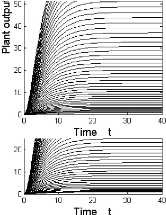
There are a lot of systems or plants in industrial processes with a monotone relation between its inputs and outputs and time inertial. The systems usually operate in a wide circumstance and are asked for multiobjective optimization. For most cases, such systems mathematical models are ill-defined, or could not be used due to some sensor limit in practice. At the controller design point, the plant information is incomplete. Such systems are very often to meet in engineering. For example, the anneal furnace heated with resistance and the water heater with gas fired for shower as well as the traction motor with heavy loads, etc. These plant outputs can

automatically reach an equilibrium state when the control inputs are fixed at some point after its inertial time. Surely that some systems can get an equilibrium point only on some specific input. For instance, a moving car only when its moving direction parallels the car body, the velocity of it can get an equilibrium point if the brake and throttle position fix. Anyway these kind of systems are the most practical in engineering and are worthy to be study in a systematic way. Before we introduce the main concept about those systems, several related terms are needed to be specified.

Considering the response function S(t,uk|u0,u1,L,un) of a plant P, if there exists a

numberδ>0 and an integer k≥0 such that S(t,uk|u0,u1,L,un) do not change when time

t∈(τ-δ, τ] or [τ, τ+δ), then τ is called an equilibrium point, and S(τ,uk|u0,u1,L,un)

an equilibr ium state of the system. Suppose that the equilibrium state only depend on the control input uk , so we denote the equilibrium state as S(uk).

Here after, if system P can reach a equilibrium state on control input point u ,

then we use S(u) to express the equilibrium state on the control input u , where t does

not appears to imply that the equilibrium state is independent to time. This part of paper is focused on the systems that can automatically reach at an equilibrium state when the control input is fixed for an enough long but a finite time.

Let Sk(t,u|u0,u1,L,un) denote the k-th component of the response function

Sk(t,u|u0,u1,L,un) starting form an equilibrium state. Let

T= sup{τ |ξ∈Ξ, u0,u1,L,un∈U,∀t> tn+τ, Sk(t,u| u0,u1,L,un)= Sk(un)}

t S t S t S t S t u (a) Output in Convex Shape (b) Output in Concave-Convex Shape (c) Output in Concave-Convex Shape (d) Output in Concave-Convex-Concave-Convex-Shape (e) step input t₀ t₀ t₀ t₀ u₀ u₁ 0 t₀ 0 0 0 0 S (t,u) S (t,u) S (t,u) S (t,u)

Fig 5.1 Sketch map of system output response shapes when input in the step change If T<∞, then call T as the maximum inertial time of Sk respective to control input

u.

Note that the inertial times of an output component vary with different control inputs. (5.1) Gives the maximum transient time from any initial state to an equilibrium state of the system. It give a time bound that we can judge or observe the performances of the system output after a control input taking into action.

Definition 5.1 . Let A(x) be a function with single

argument with domain X . We say A(x) is monotone

(strictly monotone )increasing at x, if ∃δ >0,∀x1,

x2∈N(x,δ )⊆X and x1<x2 such that

A(x1)≤A(x2)(A(x1)<A(x2))holds . Similarly, the monotone (strictly monotone) decreasing at a point of a function can be defined. A interval I⊆X is called as a monotone (strictly monotone) interval of A(x) iff

(1) A(x) has the same monotonicity (strictly

monotonicity) at any point in I.

(2) ∀x∈I , I is the maximum interval which keeps the same monotonicity and includes point x.

Definition 5.2 Let u0,u1,L,un be a step control

sequence such thatuk-1≠uk . k=1,L, n. Connecting points

(tk,uk), k=0,L,n in succession with piecewise-line, we get a

curve u=f(t), t∈[t0, tn] satisfies that uk = f(tk), k=0,L, n.

The number of monotone interval of f is called the

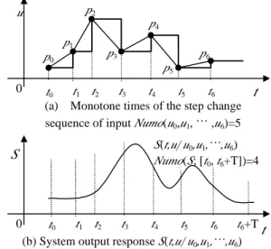
monotone times of that step control sequence ,and denoted by Numo(u0,u1, L ,un). Similarly, The number of

monotone interval of f on the interval [t0,t] is denoted by Numo(f ;[t0,t]).

Observing the systems those inputs and outputs has the relation of monotone and time inertia, we can find the

common characteristic as follows: no matter the inputs are changed continuously or step-like, the system outputs is always continuous; When the system output are moving up (or going down), any control action that make the output convert to its opposite trend is applied to the system, the output will still maintain the moving up (or going down) trend for some time; If the input changes in step with various initial states, the ordinary output response of the system are just like the cases (a), (b) and