行走區域標示及危險狀況判別之盲人輔助系統

國 立 交 通 大 學

電子工程學系電子研究所碩士班

碩

士

論

文

行走區域標示及危險狀況判別之

盲人輔助系統

Walking Area Labeling and Dangerous

Situation Detection for Visually Impaired

研究生：鄭綱

指導教授：王聖智博士

行走區域標示及危險狀況判別之

盲人輔助系統

Walking Area Labeling and Dangerous Situation Detection

for Visually Impaired

研究生：鄭綱 Student：Kang Cheng

指導教授：王聖智博士 Advisor：Dr. Sheng-Jyh Wang

國立交通大學

電子工程學系電子研究所碩士班

碩士論文

A Thesis

Submitted to Department of Electronics Engineering &Institute of Electronics College of Electrical and Computer Engineering

National Chiao Tung University in partial Fulfillment of the Requirements

for the Degree of Master in

Electronics Engineering September 2011

Hsinchu, Taiwan, Republic of China

i

行走區域標示及危險狀況判別之

盲人輔助系統

研究生：鄭綱 指導教授：王聖智博士

國立交通大學

電子工程學系電子研究所碩士班

摘要

在本論文中，我們提出一套以視覺為基礎的盲人輔助系統。本系

統採用了資料庫為主的架構，首先具有正常視力之輔助者事先於盲人

經常行走之區域，建立 360 度全景之資料庫，並對資料庫圖片事前標

籤重要的物體，像是人行道及道路；然後從全景資料庫中尋找與使用

者前方視野最相近的區域；接著把此最接近之區域的標籤利用兩張影

像之間的對應，產生目前環境的標籤；最後利用推論的標籤來判斷盲

人目前的處境是否危險。只要使用者處於有設置資料庫的環境下，本

系統能幫助盲人辨識可行走的區域，達成輔助盲人安全行走之目標。

ii

Walking Area Labeling and Danger Detection

for Visually Impaired

Student: Kang Cheng Advisor: Dr. Sheng-Jyh Wang

Department of Electronics Engineering, Institute of Electronics

National Chiao Tung University

Abstract

In this thesis, we propose a data-driven system that assists blind

people to walk safely on the sidewalk. In our system, an assistant with

normal vision is asked to create the database for the places where the

blind user usually visits. At each sampling spot of these places, the

assistant takes a few photos that cover different viewing directions around

the sampling spot to create a panorama image. After the installation of the

database, the blind user is equipped a camera while he or she is walking

around these places. For each captured image by the camera, the

proposed system finds the most similar panoramic part in the database to

identify the location and the orientation of blind user. With an

image-to-image matching to warp the labels from the matched panoramic

part to the captured image, our system can roughly infer the labeling of

the contents within the captured image. Finally, based on the inferred

labels, our system can identify situations that could be dangerous to the

blinds.

iii

誌謝

首先非常感謝我的指導教授 王聖智老師，在念研究所的期間，老師

的潛移默化之下，習得諸多理工知識，尤其是從老師身上學習到了很

多報告的技巧，以及做研究正確的方法與邏輯。謝謝老師仔細的指導，

讓我在這兩年如沐春風！再來感謝敬群學長、慈澄學長、禎宇學長、

維辰學長、家豪學長以及其他眾多實驗室學長們提供的寶貴意見，讓

我的研究更為完善。也謝謝實驗室的好夥伴：玉書、韋弘、開暘、郁

霖，以及學弟妹們。與你們相處的日子非常開心，實驗室總是充滿笑

聲，讓我覺得一點也不孤獨！最後感謝我的父母，有你們不求回報的

支持和鼓勵，我才能好好的完成課業及研究。

iv

Content

Chapter 1. Introduction ... 1

Chapter 2. Backgrounds ... 3

2.1. Ultrasonic, Laser and RFID Travel Aid Systems ... 4

2.1.1. Ultrasonic Sensors ... 5

2.1.2. Laser Sensors ... 6

2.1.3. RFID ... 7

2.2. Vision-based Travel Aid Systems ... 8

2.2.1. Landmark Targeting ... 9

2.2.2. Scene Understanding ... 11

2.2.3. Vision-based Guiding Systems ... 13

Chapter 3. Proposed System ... 16

3.1. Sub-Database Retrieval ... 18

3.1.1. Building Panoramic Database ... 19

3.1.2. Sub-Database Retrieval for Neighboring Scenes ... 20

3.2. Determination of Facing Direction ... 21

3.2.1. Global Feature: Gist ... 22

3.2.2. Spatio-temporal Constraint for Search Window ... 25

3.3. Scene Alignment and Label Transformation... 27

3.3.1. SIFT Flow ... 28

3.3.2. Panoramic Approach ... 32

3.4. Dangerous Situation Detection ... 33

3.5. Temporal Interpolation ... 37

3.5.1. Motion Prediction ... 38

3.5.2. Label Propagation ... 38

Chapter 4. Experimental Results ... 40

4.1. Label Results of Different Approaches ... 40

4.2. Outdoor Experimental Results within NCTU ... 42

4.2.1. Database Setup ... 42

4.2.2. Experimental Results in Test Environments ... 43

4.2.2.1. Results of Database Retrieval ... 44

4.2.2.2. Cloudy Day ... 45

4.2.2.3. Sunny Day and Evening Time ... 48

4.2.2.4. Experimental Data ... 49

Chapter 5. Conclusions ... 53

v

List of Figures

Figure 1-1 Some examples of dangerous situation while walking on a sidewalk. Our

goal is to identify dangerous situations based on the captured images. ... 2

Figure 2-1 Prototype of Navbelt [2]... 5

Figure 2-2 Functional components of Guide cane [3] ... 6

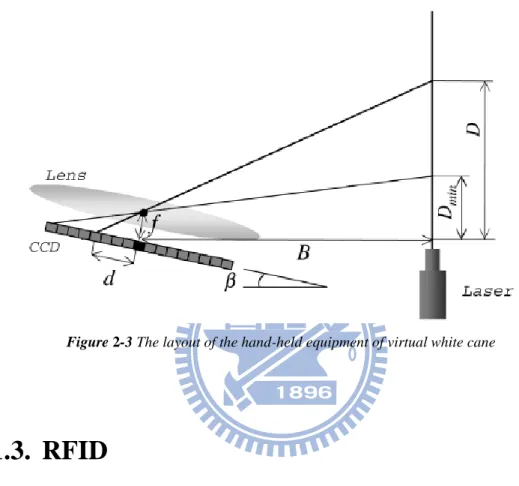
Figure 2-3 The layout of the hand-held equipment of virtual white cane... 7

Figure 2-4 The framework of the navigation system in [7] using RFID ... 8

Figure 2-5 Block diagrams of the framework in [8] ... 10

Figure 2-6 Some results of path detection in [8] ... 11

Figure 2-7 Example results from Textonboost [10] for image understanding ... 12

Figure 2-8 Example result of SuperParsing in [11] ... 13

Figure 2-9 System overview of [12] ... 14

Figure 2-10 Multi-level surface patch models for [12]. ... 14

Figure 2-11 Guiding result of [13] ... 15

Figure 3-1 Block diagram of proposed system ... 17

Figure 3-2 Major challenges: (a) variations of scene appearance, (b) feature similarity between road and sidewalk, and (c) very different scene contents from different viewing directions. ... 18

Figure 3-3 Stitching 16 images of different viewing directions to form a panoramic image. ... 19

Figure 3-4 An example of three adjacent sub-databases. Here, all the panoramic images have the same arrangement of directions. ... 20

Figure 3-5 Labels of a panoramic image ... 20

Figure 3-6 Garmin‟s USB-version GPS 18 ... 21

Figure 3-7 Different scene categories ... 22

Figure 3-8 Gabor filter banks for multiple scales and orientations ... 23

Figure 3-9 Filter bank responses ... 24

Figure 3-10 Block diagram of Gist feature extraction ... 24

Figure 3-11 Visualization of Gist feature for different image views ... 25

Figure 3-12 Slow motion of blind user reduces searching area for the panoramic images ... 26

Figure 3-13 (a) Input frame. (b) The best matched image portion. ... 27

Figure 3-14 Visualization of SIFT features ... 29

Figure 3-15 (a) Input frame. (b) Best match from database. (c) Warped image. ... 30

Figure 3-16 (a) Best match and the corresponding labels. (b) Input frame and the inferred labels... 30

vi

Figure 3-18 Illustration of poor alignment. (a) Input frame. (b) Best match. (c)

Warped image. ... 31

Figure 3-19 Panoramic extension of original support image ... 32

Figure 3-20 More information is acquired by using panoramic approach. Top: extended support image. Bottom: input frame. Color lines indicate feature correspondence ... 33

Figure 3-21 Region of interest that models human‟s visual attention area ... 33

Figure 3-22 Decision rules for direction turning ... 36

Figure 3-23 Flow diagram of dangerous situation detection ... 36

Figure 3-24 Simplified architecture by using temporal information ... 37

Figure 3-25 Camera panning caused by the turning of the user ... 38

Figure 3-26 Histogram of SIFT flow magnitudes in the horizontal direction when the user turns left. The green words indicate the inferred camera status. ... 39

Figure 3-27 Histogram of SIFT flow magnitudes in the horizontal direction when the user walks straight. The green words indicate the inferred camera status. ... 39

Figure 4-1 (a) Single-view support image, (b) panoramic-view support image, (c) warped result from single-view image, (d) warped result from panoramic-view image, (e) ground truth labels, (f) mapped labels based on single-view support, and (g) mapped labels based on panoramic view. .... 41

Figure 4-2 (a) Single-view support image, (b) panoramic-view support image, (c) warped result from single-view image, (d) warped result from panoramic-view image, (e) ground truth labels, (f) mapped labels based on single-view support, and (g) mapped labels based on panoramic view. .... 41

Figure 4-3 Our test routes in NCTU ... 42

Figure 4-4 Scene appearances ... 42

Figure 4-5 Results of database retrieval for walking forward with some pedestrians passing by. (a) Frame index, (b) input frames, and (c) the best match from the panoramic sub-database. ... 44

Figure 4-6 Results of database retrieval for a panning case. (a) Frame index, (b) input frames, and (c) the best match from the panoramic sub-database. ... 44

Figure 4-7 The case of walking forward in safe situation. (a) Frame index. (b) Input frames. (c) Inferred labels. (d) Outcome of dangerous situation detection. ... 45

Figure 4-8 The case of turning to a wrong direction. (a)Frame index. (b) Input frame. (c) Inferred labels. (d) Outcomes of dangerous situation detection. (e) Suggested turning direction. ... 46 Figure 4-9 The case of approaching to the border of sidewalk and road. (a) Frame

vii

index. (b) Input frames (c) Inferred labels. (d) Outcome of dangerous situation detection. (e) Suggested turning direction. ... 47 Figure 4-10 The case of little sidewalk area in front of the user. (a) Frame index. (b)

Input frame. (c) Inferred labels. (d) Outcome of dangerous situation detection. (e) Suggested turning direction. ... 47 Figure 4-11 Test results in sunny day. (a) Input frames. (b) Inferred label. (c) Outcome of dangerous situation detection. (d) Suggested turning direction. ... 48 Figure 4-12 Some examples at evening time. (a) Input frame. (b) Inferred labels. (c)

Outcome of dangerous situation detection. (d) Suggested turning

direction. ... 49 Figure 4-13 Ground truth definition (a) to (c): apparent cases, (d) to (f): use the

viii

List of Tables

Table 4-1 Accuracy of sub-database retrieval ... 49 Table 4-2 Definition of false positive and false negative ... 50 Table 4-3 Experimental data at cloudy day and comparison of single-view approach 51 Table 4-4 Experimental data under different lighting conditions ... 51 Table 4-5 Computational speed for our system ... 52

1

Chapter 1.

I

NTRODUCTION

For people with normal vision, taking different activities outdoors, like shopping or playing sports, is just a piece of cake. However for thousands of blind people, even walking on sidewalk safely is not a simple task. Because visually impaired people cannot see the world clearly, they may be unconscious of walking into a wrong way. In order to take a safe travel outdoors, visually impaired people usually need a white cane or a guide dog to assist them. But the tactile information passed from the end of white cane is not always robust, and a guide dog may get easily interfered by the environment. With the rapid development of vision-based technologies, one may think if there is some kind of “virtual eyes” for blind people. That is, whether we can utilize algorithms of computer vision to provide a more convenient life for blind people?

With the booming information technology in recent years, many portable devices can surf over internets and connect to global positioning system (GPS). Besides, the computational speed for portable devices is much faster than before. On the other hand, researchers have found that blind people tend to travel around places that are familiar to them. With the above two phenomena, we may be able to develop some kind of guiding system for blind people. For example, for a given environment, we can create a database beforehand. After that, when a blind user walks into this environment, he/she can use a portable device equipped with GPS to identify his/her location and to extract the corresponding information from the database to assist his/her movement within the scene.

2

In this thesis, our system is built based on the aforementioned data-driven framework. Given a video, our system automatically labels the safe walking area and determines whether the current situation is dangerous or not for the blind people. Some examples of dangerous situations are shown in Figure 1-1. Here we combine database retrieval and image-to-image dense matching to label the walking areas in a local environment. Based on the information extracted before, the system helps blind people to identify dangerous situations while walking. The red areas in Figure 1-1 represent the road regions and the green areas indicate the sidewalk regions.

Figure 1-1 Some examples of dangerous situations while walking on a sidewalk. Our goal is to identify dangerous situations based on the captured images.

In the following chapters, we will first introduce a few kinds of electronic aid systems for blind people in Chapter 2. In Chapter 3, we present the proposed system for safe area labeling and dangerous situation detection. Some experimental results will be shown in Chapter 4. Finally, we will give our conclusion in Chapter 5.

3

Chapter 2.

B

ACKGROUNDS

Because visually impaired people cannot see the world clearly, they need something to help them walk safely indoors and outdoors. Generally speaking, white canes and guide dogs are the most popular travel aids for blind people. White cane is a hand-held facility that can assist blind people to notice some drop-offs on the walking area or some obstacles in front of him/her. On the other hand, guide dogs help blind users to find the safe walking direction. For over thirty years, many technologies have been applied to develop supporting devices that assist visually impaired people to live in a more convenient way. According to [1], these technologies are classified into three categories based on their functionalities. These three categories are listed as follows.

1) Electronic travel aids (ETAs):

ETA systems help blind people to roughly know the environment. For instance, some systems can tell whether there is an obstacle in front of the user or not. Some other systems can tell when crucial objects appear near the user.

2) Electronic orientation aids (EOAs):

Because of the poor vision of blind people, they may lose the sense of direction while walking. Hence, some systems are developed to tell blind people which direction they are facing to.

3) Position locator devices (PLDs):

4

integrated in many 3C devices, like smart phones. Blind people can easily know their current location if they bring a GPS device with them.

EOA and PLD systems have been developed and widely used in the last decades. On the other hand, ETA systems have been developed over the past thirty years. In this thesis, we focus on the usage of ETA devices. In Section 2.1, we will introduce some electronics travel aid systems using ultrasonic, laser, and RFID technology. In Section 2.2, we will introduce systems using vision sensors, and introduce what kinds of functionalities can be achieved by computer vision based algorithms.

2.1. U

LTRASONIC

,

L

ASER AND

RFID

T

RAVEL

A

ID

S

YSTEMS

As the name suggests, sensor-based systems are set up by using some specific sensors, like ultrasonic sensors or laser sensors. Since 1960‟s, many evolving technologies have been proposed for the navigation aids of blind people. Ultrasonic and laser sensors are usually used to detect obstacles in front of blind people, while RFID systems can help blind people to obtain some information about the local environment.

In Section 2.1.1 we will introduce two guidance systems that use ultrasonic sensors. In Section 2.1.2, we will introduce some approaches that use lasers. In Section 2.1.3, we will introduce the RFID framework for the assistance of visually impaired people.

5

2.1.1. Ultrasonic Sensors

In the 1990s, many researchers discovered that obstacle avoidance systems for mobile robots were highly related to the guiding system for blind people. The Navbelt [2] was a typical example. The technology used in Navbelt is originally developed for mobile robot guidance. The designers claim that Navbelt enables the user to avoid obstacle safely while walking in unknown environments. Moreover, this system was implemented to be portable and its prototype is shown in Figure 2-1.

Figure 2-1 Prototype of Navbelt [2]

The Navbelt is equipped with eight ultrasonic range sensors, a portable computer, and earphones. These ultrasonic sensors are used to detect obstacles. The computer converts the received signals to an information map that records the orientations and distances to the obstacles in front of the blind user. Navbelt has two modes, image mode and guidance mode. In the image mode, the system tells a user the orientations and distances to the obstacles by using different tones and amplitudes via earphones. On the other hand, in the guidance mode; it assumes that the momentary direction and destination of user are known. Hence, the Navbelt can use the sensors signal to guide the user. However, in reality, the blind man would need an assistant with normal

6

vision to help him/her to walk for a while so the system could know the desired direction for the blind.

By the same research group, Guide cane [3] is developed as an updated version of Navbelt. This system can be held as a white cane, as shown in Figure 2-2. By detecting obstacles, it guides the user to walk along the safer way. It would be convenient to use this system and the user won‟t need too much training time to get used to the system.

Figure 2-2 Functional components of Guide cane [3]

2.1.2. Laser Sensors

When setting up a travel aid device for blind, laser sensors are another choice. Like the laser cane in [4], laser sensors are also used for obstacle avoidance. In the work of [5, 6], the authors developed a hand-held environment discovering equipment named “virtual white cane”. In their system, they use a laser-based range sensor and a CCD camera. The system layout is illustrated in Figure 2-3. When a laser beam is emitted from a laser pointer, the refection is to be detected by the well aligned CCD sensor array. When the blind user swings the hand-held equipment around, the local

7

environment information will be captured. Based on the time profile produced by the light, the equipment can analyze the data to estimate some environmental features, such as steps and drop-offs. However, for an outdoor environment, the laser may be jammed by a lot of unexpected noise.

Figure 2-3 The layout of the hand-held equipment of virtual white cane

2.1.3. RFID

For outdoor walking, visually impaired people are used to find blind tiles in order to follow them by hand-held white cane. In [7], they built a large-scale guiding framework based on Radio Frequency Identification (RFID) devices and wireless communication technology. In their framework, RFID tags, which can offer useful information provided from the centralized information system, are buried under the roads. With an RFID reader embedded in the blind cane, the blind users can get some helpful information like the status of traffic light or the location of the nearest bus station. An illustration of this framework is shown in Figure 2-4. Even though this framework provides sufficient assistance for visually impaired users, it would require

8

a lot of efforts to create such a large-scale comfortable environment.

For obstacles detection, sonar- and laser-based travel aids have boomed for many years. A major advantage of these devices is their efficient computation. However, these devices can only detect objects that have an apparent 3-D shape. For example, the signals emitted by sonar sensors are not able to detect sidewalks, curbs, or roads. Another drawback is their high cost.

Figure 2-4 The framework of the navigation system in [7] using RFID

2.2. V

ISION

-

BASED

T

RAVEL

A

ID

S

YSTEMS

As mentioned before, electronics travel aids (ETAs), which make use of ultrasonic and laser sensors, have been developed to help blind user‟s daily activities in both indoor and outdoor environments. Compared to these popular technologies, vision-based approaches can provide some other advantages. For example, image sensors, like webcams, have low cost and low power demands. In theory, one can use cameras to capture all the visual information in front of the blind user. In other words, camera can be seen as “virtual eyes” for the blind people. With this property, we can

9

develop much more fantastic functionality to help the blinds by using computer vision based algorithms.

In computer vision, object detection and recognition are crucial and challenging. Given an image, there may be some informative objects for traveling, like waymarks, crosswalks, traffic lights, and sidewalks. In recent years, some researchers have investigated the issues of automatic detection, recognition, and segmentation of multiple objects in an image. Besides, the scene understanding issue has been raised to decompose the given image into several semantically meaningful regions. If the scene understanding algorithms can roughly identify the spatial layout of the scene, this useful message can be passed to visually impaired users to help them understand their current environments.

In Section 2.2.1, we will introduce a system for landmark targeting. The system detects the prominent objects which are specific and important for blinds. In Section 2.2.2, we will introduce a few state-of-the-art scene understanding algorithms. These works may achieve multi-class object segmentation and labeling. In Section 2.2.3, we will introduce some vision-based guidance systems.

2.2.1. Landmark Targeting

While taking a walk outdoors, we usually follow sidewalks for the concern of safety. On the other hand, we also need to pay attention to some obstacles such as cars and people to avoid collision. In [8], the authors proposed a cheap and wearable facility for visually impaired people. The block diagram of the overall system is illustrated in Figure 2-5.

10

Figure 2-5 Block diagrams of the framework in [8]

In their system, they first search the paths in the input frame. The path detection window is initially set to be under a horizontal line that is close to the middle of the frame. After the initial frame, the position of the horizontal line is updated dynamically based on the detected path borders and the corresponding vanish points of previous frames. After that, the Canny edge detector is used to generate an edge map. In their approach, the authors assume the shape of the path in front of the user is simple. Hence, the gradient orientations of the sidewalk borders are restricted to a certain range. Besides, they assume the borders would intersect at a vanish point. Based on the above assumptions, Hough transform is used to search for lines within the path detection window. Some path detection results are shown as Figure 2-6. After path detection, edge and texture cues are utilized to detect static obstacles. Moreover, the optical flow method is used to capture moving obstacles such as human walking on the sidewalk. Finally, the stereo disparity can provide the distance information of the detected obstacles. Since the edge and texture cues can easily get interfered by occlusion or shades, their work is currently limited to simple scenes only.

11

Figure 2-6 Some results of path detection in [8]

2.2.2. Scene Understanding

In current multi-class object recognition/segmentation algorithms, Markov random field (MRF) or conditional random field (CRF) [9] is usually adopted to incorporate different features in a single model. In [10], they proposed an approach to learn a discriminative model of object classes which combines texture, layout, and context information efficiently. They also use conditional random field to learn and combine texture-layout, color, location, and edge cues in a unified model, as expressed in Eq. 2-1. Here, the notation c indicates the class label and x indicates the image. ( , ) log ( | , ) ( ( , ; ) ( , ; ) ( , ; )) ( , , ( ); ) log ( , ) i i i i i i i j ij i j P c c x c i c c Z                     





In this equation, the first term is texture-layout potentials; the second term is color potentials; the third term represents location potentials; the fourth term is edge potentials that measure the class located in the two sides of the edge; and Z is the partition function term to normalize the distribution. In the training stage, they want to learn the weighting θ for each feature term. In the label inference stage, they apply the learned model to the image and try to associate object category label with pixels or

12

other image representations (see Figure 2-7). Finally, the input image is partitioned to semantic meaningful regions. However, there may be some drawbacks in these learning-based methods. One is that it is hard to adjust the number of object categories after the model is determined. Moreover, if the features of different object classes are similar, the inference results may be wrong.

Figure 2-7 Example results from Textonboost [10] for image understanding

On the other hand, the authors in [11] adopted a data-driven approach. They first retrieve similar scene type from the retrieval set and generate super-pixels for the query image by using bottom-up segmentation. The super-pixels are described by shape, location, texture, and appearance features. After those two steps, the likelihood ratio score of object classes for each super-pixel can be obtained. They encode contextual constraints with the help of Markov random field, as expressed in Equation 2-2. Here, c also denotes the class label and si represents the ith super-pixel. For each

semantic class is associated with a geometry class, such as ground, sky, or vertical. Finally they jointly determine the geometric labels and semantic labels by optimizing the objective function in Equation 2-3, which is an extension of Equation 2-2. Here,

13

the notation g represents geometric class label. The last term of Equation 2-3 enforces the coherence between geometric class and semantic class. This term is zero when these two labels are matched correctly, and is one otherwise. An example is shown in Figure 2-8. ( , ) ( ) ( , ) ( , ) i i j data i i smooth i j s SP s s A J E s c  E c c   







Figure 2-8 Example result of SuperParsing in [11]

2.2.3. Vision-based Guiding Systems

In [12], the authors proposed a wearable and stereo-vision based navigation system for blind people. A pair of cameras is used as the data acquisition device. They also combine visual odometry and Simultaneous Localization and Mapping (SLAM) algorithm into their work. By utilizing camera pose estimation with dense 3D information from stereo-vision, a vicinity map is created for the surrounding environment. The block diagram of their system is illustrated in Figure 2-9.

14

Figure 2-9 System overview of [12]

However, the main limitation of their work comes from the stereo-vision architecture. When the local environment is low-textured, the depth map produced by the stereo camera system will not be accurate enough. Some surface model results are shown in Figure 2-10, where red regions represent vertical surfaces, green regions represent horizontal surfaces, and the red cones represent camera orientations.

15

In [13], the authors proposed a data-driven framework. In their system, training video sequences were taken beforehand. They select some key frames as reference data and perform registration with respect to 2D positions and orientations. For every key frame, they extract Speeded Up Robust feature (SURF) [14] and GIST feature [15]. When the query image is captured, the user will know where he/she is by matching feature to the reference images in the database. The scene continuity is modeled by the hidden Markov model (HMM). The guiding result is shown in Figure 2-11, where black dots represent key frame locations, blue lines represent ground truth location of query frames, green lines represent covered ground truth, and red parts represent the locations where error is over ten meters from the ground truth. For outdoor cases, using GPS tools can achieve faster and more accurate localization than the proposed method in [13].

16

Chapter 3.

P

ROPOSED

S

YSTEM

While traveling outdoors, walking on the sidewalk is the commonest action. For people who have normal vision, it‟s easy to change momentarily the walking direction to avoid dangers. However, for thousands of blind people, they are afraid of walking in a wrong direction, which may cause fatal dangers to them. Hence, automatically detecting the walking area in front of blind people could be very helpful to them. For blind people, the white cane is a commonly used tool. However, white canes cannot provide reliable tactile information to help blind users distinguish curb from sidewalk. On the other hand, the state-of-the-art sonar- and laser-based systems cannot detect the unobvious drop-offs on the sidewalk borders in outdoor environments either. To achieve this kind of assistance, we aim to utilize computer vision algorithms.

Up to now, some nowadays popular scene understanding algorithms learn a model to classify different image regions into corresponding object categories. However, due to the multiple outdoor scene appearances and the view-dependent variations of scene structure, a single model may not be able to efficiently handle the scene understanding problem. Moreover, the scene understanding algorithms may get poor inference results when the features of different objects appear to be similar.

From the habit investigation of blind people, we learn that blind people are used to walk around in an environment that they are familiar with. This phenomenon inspires us to adopt a data-driven approach. On the other hand, many modern portable devices are able to surf over the internet and to receive GPS signals to identify their geographic locations. Hence, we can set up a database for the places where the blind

17

user tends to visit. When the blind user walks around these places, he or she can use the information captured by his/her portable device and the identified geographic location to retrieve appropriate reference data from the already installed database in order to achieve safer navigation.

In this thesis, the goal of our system is to label the walking area for the current scene in front of the blind user. First, the blind user will use some geographic locating device like GPS to identify his/her current location. Based on the current location, the system retrieves a few panorama images from the database to represent the neighboring scenes of the blind user. After that, with respect to the image captured by the portable camera hung in front of the blind user, the system adopts a fast global feature matching method to search within the panoramas the most similar scene. In practice, the captured image and the matched image data would be roughly the same. Since we have already labeled some important objects, like roads and sidewalks, in the panorama images, we can warp the labels of the matched image to form the labels of the captured image. With the mapped labels, the system can roughly understand the current scene in front of the user and detect some situations that could be dangerous to the user. Figure 3-1 shows the block diagram of our framework.

18

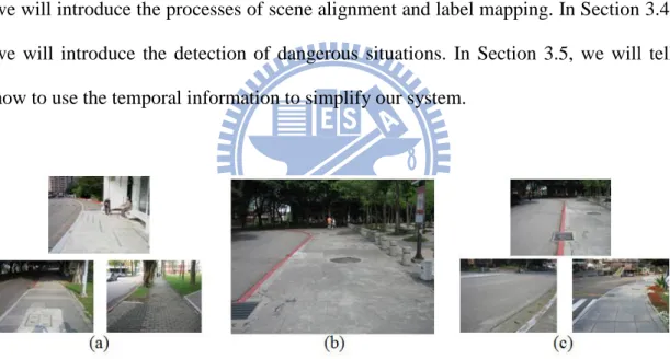
The challenges of our system includes: (1) the scene appearance may vary a lot in an outdoor environment; (2) the features of road and sidewalk may be similar to each other; and (3) the observed scene may vary a lot with respect to different viewing directions. Some examples of these challenges are shown in Figure 3-2.To solve the first and second challenges, we adopt a database retrieval approach to search for the most similar image that interprets the surrounding scene. To solve the third challenge, the database is composed of panoramic images. In Section 3.1, we will explain the detail of database construction and sub-database retrieval. In Section 3.2, we will introduce the algorithm that determines the facing direction of the user. In Section 3.3, we will introduce the processes of scene alignment and label mapping. In Section 3.4, we will introduce the detection of dangerous situations. In Section 3.5, we will tell how to use the temporal information to simplify our system.

Figure 3-2 Major challenges: (a) variations of scene appearance, (b) feature similarity between road and sidewalk, and (c) very different scene contents from different viewing directions.

3.1. S

UB

-D

ATABASE

R

ETRIEVAL

In this section, we will introduce how to build the database and how to retrieve the sub-database that contains the panoramic images of the neighboring scenes.

19

3.1.1. Building Panoramic Database

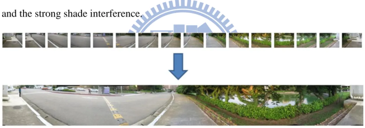
In order to safely walk around in the campus of National Chiao Tung University, we should set up a database that represent the scenes around a few sampling spots in the campus. In the following paragraphs, we will explain how we install the database. At each sampling spot, we took photos at 16 different viewing directions to model the possible views that a person with normal vision may see. These 16 photos were stitched together to form a 360-degree panoramic image, as shown in Figure 3-3. When we took the photos, our camera is held at about 1.6 meters height. Moreover, we took these photographs in cloudy days in order to reduce the strong-light effect and the strong shade interference.

Figure 3-3 Stitching 16images of different viewing directions to form a panoramic image

To stitch these photos of different viewing directions, we use the Hugin panorama creator, which allows several overlapping photographs taken at the same place to be merged into a large photo. This panorama creator matches the Scale Invariant Transform (SIFT) features of the overlapping regions of two images to align and transform photos to create a panoramic image. Before stitching images, we have to choose an anchor image at a certain direction to achieve the same arrangement of the panorama while stitching, as shown in Figure 3-4. The white balance and exposure are also corrected for each image based on the anchor image.

20

Figure 3-4 An example of three adjacent sub-databases. Here, all the panoramic images have the same arrangement of directions.

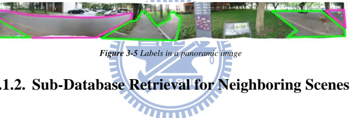
After having obtained the panoramic images, we label each panorama to create the annotations. Here, we use the on-line labeling tool LabelMe [16] to label the important regions such as sidewalks and roads in the panorama, as shown in Figure 3-5. Inside the green polygons are labeled as sidewalk regions, while inside the pink polygons are labeled as road regions.

Figure 3-5 Labels in a panoramic image

3.1.2. Sub-Database Retrieval for Neighboring Scenes

To interpret the surrounding environment for the user, we don‟t need to search over the whole database but only need to check a local sub-database. Intuitively, there may be some degree of scene discontinuities between adjacent sub-databases. Hence, we may not be able to get good interpretation of the surrounding environment if we only check the nearest panoramic image. Moreover, the routes in campus are not always straight. Hence, the scene at some sampling spots may have complex spatial layout. To deal with these problems, we search the panoramic images at three nearby sampling spots.

Our system is a kind of wearable aid system for visually impaired user. In real implementation, we use a GPS device to find user‟s location. Here we use the Garmin

21

GPS 18portable device, as shown in Figure 3-6. Garmin GPS 18 updates the location for every second and has a USB connection that can be easily connected to wearable equipment. When this device is connected to a notebook, we use the open source software Franson GpsGate 2.6 to extract NMEA data from the device to get the current latitude. Like in [17], we have tagged all of our panoramic images with the corresponding GPS coordinates. Hence, by using the Garmin GPS 18 to get the current GPS location, we can identify the three panoramic images that have the shortest geographic distance with respect to the current location. These three panoramic images are treated as the sub-database for subsequent processes.

Figure 3-6 Garmin’s USB-version GPS 18

3.2. D

ETERMINATION OF

F

ACING

D

IRECTION

After finding the sub-database of three panoramic images at nearby sampling spots, as shown in Figure 3-4, we search within each panoramic image to find the image portion that is most similar to the current front-view image of the user. This action can be seen as modeling the “virtual sight” for visually impaired people. With the matched image portion, the blind user will be able to roughly know the current

22

direction he/she is facing to.

In this step, we want find the most similar part efficiently via feature matching. Many popular image matching algorithms in the literature, such as SIFT or Speeded Up Robust Feature (SURF), are developed to match local regions. With these approaches, the matching result may get easily interfered by unexpected objects in the scene, like walking people or cars. In our approach, we describe the whole image in terms of a single global feature vector, by which we can achieve lower computational complexity and lower noise interference.

In the literature, global features are usually used to solve scene categorization problems. Different scene categories usually have different appearances, as shown in Figure 3-6. For example, street scenes may contain lots of vertical and horizontal lines, while natural scenes usually contain undulating contours. In our case, we want to utilize a global feature to search for the matched image portion in the panoramic images. For every panoramic image in the sub-database, we partition it into 32 overlapping sub-images along the horizontal direction. Hence, given the image captured by the camera, we try to find the best match among the 32 (sub-images per panorama) 3 (panoramas per sub-database) = 96 sub-images. In Section 3.2.1, we will introduce the widely used global feature “gist”. In Section 3.2.2, we will introduce how to model the blind‟s slow motion in the global matching process.

Figure 3-7 Different scene categories

3.2.1. Global Feature: Gist

23

to human eyes from different spatial regions of an image. In other words, the gist feature models coarsely the edge and texture information of different spatial regions in an image. This feature has been tested for various kinds of applications, like scene categorization and image retrieval, and has demonstrated reliable performance. Moreover, with the low dimension of this feature, we can efficiently measure the similarity between two images.

The gist descriptor performs Fourier transform analysis after the pre-processing that reduces boundary artifacts and normalizes the local contrast. To construct the gist feature, the image is convolved with a multi-scale oriented Gabor filter bank, as shown in Figure 3-8.The Gabor filter bank is composed of four scales, with each scale having eight orientations. The filter bank responses are shown in Figure 3-9.

24

Figure 3-9 Filter bank responses

Next, for each filter output, we average the magnitude response within each 44 non-overlapping blocks of the image. These responses are stacked together to form a 4448=512 dimensional feature vector. The overall flow chart of the gist feature extraction is shown in Figure 3-9.

Figure 3-10 Block diagram of Gist feature extraction

On the other hand, our panoramic image is composed of 16 images of different directions to cover the 360-degree view of a scene. For different viewing directions, the scene structure could be very different and the statistics of detected edges and the texture representation are different. In Figure 3-11, we show the visualization of gist features in polar plots, where along the radius green and red colors are used to

25

represent different responses of multi-scale filters. Filter responses of different orientations are encoded in different angles of the polar plots. The brightness of the color represents the magnitude of the response. The 16 polar plots indicate the filter responses of the 16 non-overlapping local image regions. In Figure 3-11, we can easily distinguish the difference of gist feature among different images. In our system, the gist feature of each sub-image in the panoramas is pre-calculated to reduce the computation time. To measure the similarity between two images, we calculate the correlation of their corresponding gist features. If we denote p as the index of the 96 sub-images, Xp as the pth sub-image, and G(I) as the gist feature of the input frame,

we find the best match Xp based on the following equation

* arg min ( ) ( ) p p p X X  G I G X  _{Eq. 3-1}

Figure 3-11 Visualization of Gist feature for different image views

3.2.2. Spatio-temporal Constraint for Search Window

In our system, we assume that the blind user don‟t move drastically. That is, the panning speed and the walking speed are not too fast. With the slow motion assumption, the orientation of the matched sub-image at the current moment will be very similar to the orientation of the matched sub-image at the previous moment. As

26

shown in Figure 3-12, if the image portion between the red dash lines represents the best match for the previous input frame, then the orange region indicates the possible image portions for matching at the current moment. This assumption can greatly reduce the search range within the sub-database. In mathematics, this concept can be modeled as a Markov chain, as expressed in Equation 3-2. Here, Pr(Xt= i) denotes the

probability at Time t that the best matched image portion is the ith sub-image in the sub-database.

, 1

Pr(Xt  j) pr jPr(Xt r) Eq. 3-2

where pij Pr(Xt  j X| t1 r) Eq. 3-3

For the implementation detail, we search for the 7 nearest directions out of all 32 directions based on the direction of the previous best match. After global feature matching, we obtain the current facing direction of the user. The matched portion of the panoramic image also roughly interprets the surrounding environment.

27

3.3. S

CENE

A

LIGNMENT AND

L

ABEL

T

RANSFORMATION

As mentioned above, we have found the image portion of the panoramic images in the sub-database that is the most similar to the front view of the blind user. Here, we call this best matched image portion as the reference image of the input frame. As a matter of fact, there still exist some differences between the input frame and the best match, as shown in Figure 3-13. That is, even though these two images are captured at similar places with similar facing directions, the scene contents are not exactly the same. Hence, we need to further align the best match with the input frame to obtain more accurate labeling results.

(a) (b)

Figure 3-13 (a) Input frame. (b) The best matched image portion.

For the sake of mapping the best match to the input frame, we focus on finding the correspondence between the two images. Up to now, many state-of-the-art methods have discussed this correspondence problem. One approach is to find some interest points of the images for matching, such as SIFT feature points. However, this sparse approach tends to have poor results when there are no appropriate interest points in the images. Another approach is to use the correspondence of regions to match the images, such as the approach in [19]. In this kind approach, they first

28

segment the images into many sub-regions. After that, they use some suitable features of the sub-regions to match the images. Intuitively, the matching result will be not accurate if the sub-regions are not accurately segmented.

In our approach, we adopt pixel-wise matching. Although the result of pixel-level matching is usually noisy, we can utilize some robust feature to tackle this problem. Here, we use SIFT flow proposed in [20] to perform pixel-wise matching in order to obtain better scene alignment.

3.3.1. SIFT Flow

SIFT flow is a novel method for the application of scene alignment. It adopts the same computational framework of optical flow to achieve dense matching. Instead of using RGB values and gradient information to represent the pixels, SIFT flow uses pixel-wise SIFT feature instead. Since this kind of histogram-based features contains contextual information around the pixel, we can use them to obtain more reliable matching results across different scene appearances. Moreover, the SIFT descriptor performs well under luminance variations of outdoor environment.

To better observe the generation of SIFT feature map, we adopt the visualization method shown in Figure 3-14. In this representation, after principal component analysis (PCA), the top three principal components of the 128-dimensional SIFT descriptors are calculated and are projected into the RGB space for visualization. In Figure 3-14, pixels with similar colors would share similar local image structure.

Even though we only use the top three principal components of the SIFT features for visualization, we use the 128-dimensional SIFT descriptors for dense matching. The objective function of the matching process is expressed as below:

29 1 2 1 ( , ) ( ) min( ( ) ( ( )) , ) ( ( ) ( ) ) min( ( ) ( ) , ) min( ( ) ( ) , ) E s s t u v u u d v v d            







Here, p and q are pixel coordinates. The notation s indicates the SIFT image and w indicates the flow vectors. The first term in Equation 3-4 is the feature matching

term, also known as the data term. In this term, SIFT features are matched across the two images. The second term sets a constraint that the flow magnitude should not be too large, with η representing the weighting of this constraint. The third term models the spatial regularization so that the flow vectors of adjacent pixels will be similar, with α representing the coefficient of flow discontinuity. The dual-layer loopy belief propagation [21] is adopted to obtain the optimized flow field, which allows the separation of the vertical flow from the horizontal flow in message passing by decoupling the smoothness term.

Figure 3-14 Visualization of SIFT features

After the optimization process, we obtain the SIFT flow field. Based on the flow vectors, we can warp the pixels of the best matched image for image alignment. As shown in Figure 3-15, the warped image will be quite similar to the input image frame.

30

Figure 3-15 (a) Input frame. (b) Best match from database. (c) Warped image.

Similarly, we map the labels of the best matched image along the flow vectors. The mapped label can be taken as the inference of the environment, as shown in Figure 3-16, where the green labels represent the sidewalk area and the red labels represent the road area. To keep the completeness of region and to suppress some outliers, we actually have performed the morphological “open” operation after the mapping of labels.

Figure 3-16 (a) Best match and the corresponding labels. (b) Input frame and the inferred labels.

As mentioned above, based on pixel-wise matching, we can map the labels of the best matched image to interpret the contents of the input image frame. The reasons why we don‟t use optical flow for dense correspondence are as follows. First, the assumption for optical flow doesn‟t fit our problem. Most optical flow methods are

31

used to describe the temporal correspondence of two successive frames in a video sequence. Due to the significant similarity between two successive frames, the assumption of consistent brightness is usually used and a small search window is usually adopted. For our case, however, there always remains certain appearance difference between the best matched image and the input frame. Hence, the traditional optical flow method may not be appropriate for our situation. Moreover, the SIFT flow approach utilizes a larger search window so that we can tolerate larger differences between these two images in scene alignment, as shown in Figure 3-17.

Figure 3-17 Different size of search window for optical flow and SIFT flow

To build meaningful correspondence between two images, we assume that these two images share a similar local image structure. The perspectives of the images are also assumed to be similar. However, the blind user may have various kinds of movement while walking on the sidewalk, such as a horizontal move shown in Figure 3-18. Under this example, the SIFT flow may not be able to perform meaningful correspondence due to the different perspective caused by the horizontal move.

32

In the above example, even though these two images are taken at the same place, we still can‟t obtain a convincible flow field to represent the matching relation. Because of the insufficient information provided by a single support image, the mapped image is not very similar to the input frame.

3.3.2. Panoramic Approach

To provide a more accurate warping result, instead of taking a single support image for dense matching, we utilize a larger image portion in the panoramic image, as shown in Figure 3-19. The extended support image is about 2.5 times wider than the width of the input frame, but with the same height. Moreover, to search over a wider support image, we also relax the constraint of flow magnitude. The weighting of flow constraint is set to 0.4 times of the original setup. With the extended support image and the relaxed flow magnitude constraint, more panoramic information can be acquired for better dense matching, as shown in Figure 3-20.

33

Figure 3-20 More information is acquired by using panoramic approach. Top: extended support image. Bottom: input frame.

Color lines indicate feature correspondence

3.4. D

ANGEROUS

S

ITUATION

D

ETECTION

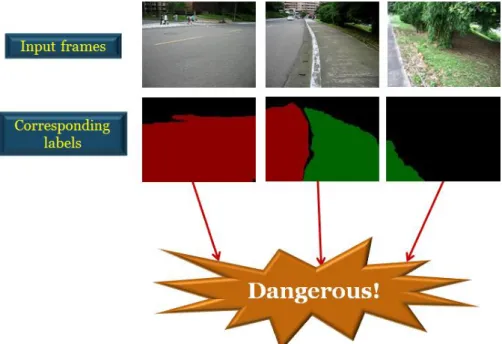
By using the inferred labels, we can decide whether the situation in front of the blind user is dangerous or not. Here we focus on the relation between road and sidewalk and apply a rule-based method to analyze these labels. Since humans typically pay more attention to the central region in front of them, we define the region of interest to be the trapezoid mask shown in Figure 3-21.

Figure 3-21 Region of interest that models human’s visual attention area.

The complete flow diagram of dangerous situation detection is illustrated in Figure 3-23. The first dangerous situation is defined to be the case when the road

34

region is larger than the sidewalk region in the trapezoid mask. This situation usually occurs when the user turns his/her direction toward the road or when the user‟s position is near the border between road and sidewalk. Here, we define the area of road label inside the mask as Ar and the area of sidewalk label as As. As expressed in

Equation 3-5, when the area ratio Aratio1 = Ar/As is larger than a certain threshold

Tharea1, we infer the situation as dangerous. In our system, Tharea1 is empirically set to

0.325.

On the other hand, the blind user may walk to the border between the sidewalk and some region other than road. For this case, we denote the unlabeled region as “undefined” and denote its area as Aun. As expressed in Equation 3-5, when the ratio

Aratio2 = Aun/As is larger than another threshold Tharea2, we infer that situation to be

dangerous too. In our system, the threshold Tharea2 is empirically set to 0.8.

1 1 2 2 1 1 1 , if , if , otherwise

=1

=1

=0

After analyzing the area ratio of different labels, we check whether the sidewalk region is right in front of the user. In other words, even if the area ratios are lower than corresponding threshold, the situation would be dangerous if there is no sidewalk label at the bottom of the trapezoid mask. Here, we infer the situation as dangerous if there is no sidewalk label within the bottom 15% region of the trapezoid mask. Here, we denote this bottom 15% region as Mb, as expressed in Equation 3-6.

35 1 2 1 2 =0 in 0 1, if & 0 0, otherwise but s Mb D A D D D   _     Eq. 3-6

The other dangerous situation happens when the sidewalk area in front of the user is too small. Here, we detect this situation if the area of sidewalk label in the mask is under a certain rate Rs, as expressed in Equation 3-7. We define AT as the area

of trapezoid mask. In our system, Rs is empirically set to be 0.25.

2 3 2 3 0 1, if & 0 0, otherwise but s s T D A R A D D D   _       Eq. 3-7

Hence, we detect the situation is dangerous if D1, D2, or D3 is one. Otherwise, the

situation is safe. After analyzing the label, the system can pass the message to the blind user so that he/she can know whether his/her current situation is dangerous or not. In real implementation, one can use an audio device to warn the blind user if he/she has the normal sense of hearing.

In addition to the detection of the dangerous situations for blind people, our system can also suggest the blind user the right direction of safe walking. After a dangerous situation is detected, we analyze the spatial layout of the warped labels to determine the right direction. In detail, we extract the pixel positions of each label class and average the coordinates of the horizontal component. If we define the center of the x coordinate of the road labels is Cr and the center of the x coordinate of the

sidewalk labels is Cs, we can compare the values of Cr and Cs to determine the

suggested turning direction. If there is no road label, we just check whether Cs is on

the right half or on left half of an image. If the area of sidewalk labels is too small, the spatial layout of labels would be unreliable. In this case, we estimate the safe direction by using the label information at the previous moment. In Figure 3-22, we present the

36

pseudo code of the decision process.

Figure 3-22 Decision rules for direction turning

37

3.5. T

EMPORAL

I

NTERPOLATION

In order to reduce the computational complexity, another approach is to utilize temporal information. Instead of performing the whole process for every frame, we can use temporal correspondence to simplify the process. In our system, we perform the whole process only over a few frames, named the anchor frames. For each anchor frame, we perform sub-database retrieval and calculate SIFT flow to generate the outcome. For those frames between a pair of adjacent anchor frames, we simply propagate the labeling results of the anchor frame to estimate their labels. This process is illustrated in Figure 3-24 below.

On the other hand, the camera may pan when the blind user turns left or right, as shown in Figure 3-25. For this case, we track the camera status using the statistics of the SIFT flow between adjacent frames.

38

Figure 3-25 Camera panning caused by the turning of the user.

3.5.1. Motion Prediction

As mentioned above, to deal with the panning of camera, we analyze the SIFT flow between two adjacent frames. Again, because of the larger search window used in the calculation of SIFT flow, we will be able to handle a large motion. To predict the motion, we analyze the flow field in the horizontal direction. Here, we calculate the mean of the flow magnitude along the horizontal direction. This result indicates the turning direction of the user. As shown in Figure 3-26 and Figure 3-27, we take the histogram of the flow magnitude in the horizontal direction. When the mean of the horizontal flow magnitudes is lower than -20, we infer the user as turning left. On the other hand, when the mean value is larger than 20, we infer the user as turning right. Some examples are shown below in Figure 3-26 and Figure 3-27.

3.5.2. Label Propagation

As mentioned above, we use temporal information to propagate the labels for non-anchor frames. The labeling results of the preceding frame are warped to generate the labels of the current frame based on the temporal correspondence between these two frames. The use of temporal correspondence makes the labeling results reliable and accurate as long as we have obtained correct labels in the anchor frame.

39

Figure 3-26 Histogram of SIFT flow magnitudes in the horizontal direction when the user turns left. The green words indicate the inferred camera status.

Figure 3-27 Histogram of SIFT flow magnitudes in the horizontal direction when the user walks straight. The green words indicate the inferred camera status.

40

Chapter 4.

E

XPERIMENTAL

R

ESULTS

In this chapter, we will demonstrate some of our experimental results. In Section 4-1, we will show the results of label transformation by the SIFT flow with single view approach and by the SIFT flow with panoramic approach. In Section 4-2, we will show the performance of our system over a real outdoor environment in NCTU. Our proposed system is tested over a personal computer with Intel® Core™ i5-760 CPU at 2.8G Hz. Our algorithm is developed in Matlab but without code optimization.

4.1. L

ABEL

R

ESULTS OF

D

IFFERENT

A

PPROACHES

First, we show the warping and label results by SIFT flow with the single-view approach and with the panoramic approach. A result is shown in Figure 4-1, which shows that the panoramic approach provides more accurate warping and label result. The parameters of SIFT flow are set to be the same for both cases. The input frame is captured at the resolution of 640480 pixels and then down-sampled to 160120 pixels. The panoramic image is 2.5 times wider than the input frame, but with the same height.

41

Figure 4-1 (a) Single-view support image, (b) panoramic-view support image, (c) warped result from single-view image, (d) warped result from panoramic-view image, (e) ground truth labels, (f) mapped labels based on single-view support, and (g) mapped labels based on panoramic view.

Another example is shown in Figure 4-2. Via panoramic approach, even though the results of warped image and label do not perfectly resemble the input frame, the results can still well represent the input frame.

Figure 4-2 (a) Single-view support image, (b) panoramic-view support image, (c) warped result from single-view image, (d) warped result from panoramic-view image, (e) ground truth labels, (f)mapped labels based on single-view support, and (g) mapped labels based on panoramic view.

42

4.2. O

UTDOOR

E

XPERIMENTAL

R

ESULTS

WITHIN

NCTU

4.2.1. Database Setup

Our system is tested on two routes near the north gate of National Chiao Tung University (NCTU), as shown in Figure 4-3. Red lines indicate these two routes, which consist of various kinds of scenes, such as bus station, intersection, or trees, as shown in Figure 4-4. The total length for these two routes is about 300 meters.

Figure 4-3 Our test routes in NCTU.

43

To create the database along these two routes, we choose 11 sampling spots in total. The selection of sampling spots is based on three criteria: 1) a scene that contains an intersection, 2) a scene that contains informative landmarks, such as crosswalk and waymark, and 3) a scene that contains special construction, like bus station. We follow these criteria to build our panoramic database. As aforementioned in Section 3-1-1, we take 16 photographs of different views at each sampling spot to create the panoramic image.

4.2.2. Experimental Results in Test Environments

We test our system over three video sequences that were captured in three different weather conditions: cloudy days, sunny days with some unexpected shadows in the scene, and evening time with low lighting condition. Here we show some inferred label and detected dangerous situations. The resolution of the videos is 640480. The test procedure of our system includes the panoramic approach and temporal interpolation mentioned in Section 3.3.2 and Section 3.5. The test video of the sunny situation was captured around 14:00 in the afternoon, while evening video was captured around 18:00 in the evening. While taking these video sequences, we mimicked the way blind people take a straight walk until the „real‟ dangerous situation occurs. Hence, the walking tracks follow a zigzag style. We sample all the test video with the sampling period of 0.6 seconds. For every 6 seconds, we pick an anchor frame. In our experiments, the detection process is performed over the anchor frames only. For the remaining frames between anchor frames, we use temporal information to propagate labels.

44

4.2.2.1. Results of Database Retrieval

In Section 3-2, we have discussed how to find the portion of panoramas which is most similar to the sight in front of the blind user. Here we show some examples of the best matches after sub-database retrieval by using gist feature matching with the spatio-temporal constraint.

Figure 4-5 Results of database retrieval for walking forward with some pedestrians passing by. (a) Frame index, (b) input frames, and (c) the best match from the panoramic sub-database.

In the previous example, we can see that the interference in the local image structure, such as passing pedestrians, doesn‟t affect the outcome of database retrieval too much. The best matched part and input frame would share a similar local structure. In comparison, in the following example, we show the case of a panning view.

Figure 4-6 Results of database retrieval for a panning case.

(a) Frame index, (b) input frames, and (c) the best match from the panoramic sub-database. .

45

4.2.2.2. Cloudy Day

For the test video captured in a cloudy day, its lighting condition is very similar to that in our database. Some results of the cloudy-day case are shown below. Here, we show different walking situations on the sidewalk and the detected dangerous situations. To visualize the outcome of our system, we use an exclamation mark to represent the occurrence of dangerous situation. Moreover, the yellow arrow indicates the suggested safe way to turn if a danger situation is detected. The case of walking forward is shown in Figure 4-7.

Figure 4-7 The case of walking forward in safe situation. (a) Frame index. (b) Input frames. (c) Inferred labels. (d) Outcome of dangerous situation detection.

Next, we show an example in which the blind user turn into a wrong direction. In this case, our system will warn the user the detection of a dangerous situation. In this example, the system informs the user to turn right to achieve safe walk.