Cycle embedding in faulty wrapped butterfly graphs

Cycle Embedding in Faulty Wrapped Butterfly Graphs

Chang-Hsiung Tsai

Department of Computer Science and Information Engineering, Dahan Institute of Technology, Hualien, Taiwan 971, Republic of China

Tyne Liang, Lih-Hsing Hsu

Department of Computer and Information Science, National Chiao Tung University, Hsinchu, Taiwan 300, Republic of China

Men-Yang Lin

Department of Information Science, National Taichung Institute of Commerce, Taichung, Taiwan, Republic of China

In this paper, we study the maximal length of cycle embedding in a faulty wrapped butterfly graph BFnwith at most two faults in vertices and/or edges. When there is one vertex fault and one edge fault, we prove that the maximum cycle length is n2n_{ⴚ 2 if n is even and n2}n_ⴚ 1 if n is odd. When there are two faulty vertices, the maximum cycle length is n2n _{ⴚ 2 for odd n. All these} results are optimal because the wrapped butterfly graph is bipartite if and only if n is even.© 2003 Wiley Periodicals,

Inc.

Keywords: Hamiltonian cycle; wrapped butterfly; fault-toler-ant; cycle embedding; Cayley graph

1. INTRODUCTION

The performance of a distributed system is significantly determined by its network topology. The hypercube (binary

n-cube) is one of the most popular interconnection

net-works. It has been used to design various commercial mul-tiprocessor machines. One basic drawback with hypercubes is that the vertex degree increases with the number of vertices. Among all networks with fixed degrees, the wrapped butterfly network is one of the most promising networks due to its nice topological properties. On the other hand, the cycle network contains several attractive proper-ties such as simplicity, extensibility, and feasible implemen-tation. Hence, embedding a cycle into a wrapped butterfly

network has received many researchers’ efforts in recent years [1, 3, 6, 8].

To embed a cycle into a faulty butterfly network BF_n

with n2n vertices, it is desirable to isolate those faulty components from the remaining ones so that a maximal-length cycle can be still embedded. Vadapalli and Srimani [6] proved that there exists a cycle of length n2n⫺ 2 when there is one vertex fault and there is a cycle of length n2n ⫺ 4 when two vertex faults occur. In [3], Hwang and Chen

showed that the maximal cycle of length n2n can be

em-bedded in a faulty wrapped butterfly graph which has two edge faults. For all integer nⱖ 3, these results are optimal because the wrapped butterfly graph is bipartite if and only if n is even.

In the previous two studies, faults are limited to either vertex faults or edge faults. However, faults in both vertices and edges may occur. Consequently, we are motivated to explore the embedding feasibility in the faulty wrapped butterfly graph. In this paper, when there is one vertex fault and one edge fault, we prove that the maximum cycle length is n2n⫺ 2 if n is even and n2n⫺ 1 if n is odd. When there

are two faulty vertices, the maximum cycle length is n2n

⫺ 2 for odd n. All these results are optimal because the wrapped butterfly graph is bipartite if and only if n is even. In Table 1, we summarize all the results about faulty edges and/or vertices in BFn.

In the following section, we discuss some properties of wrapped butterfly graphs. In Section 3, we prove that the faulty wrapped butterfly graph contains a cycle of length

n2n ⫺ 2 if it has one vertex fault and one edge fault.

Finally, when n is an odd integer, we prove that the wrapped butterfly graph contains a Hamiltonian cycle if it has at most two faults and at least one of them is a vertex fault.

Received October 2000; accepted April 2003

Correspondence to: C.-H. Tsai; e-mail: chtsai@ms01.dahan.edu.tw

Contract grant sponsor: National Science Council of the Republic of China; contract grant number: NSC 89-2115-M-009-020

2. WRAPPED BUTTERFLY GRAPHS AND THEIR PROPERTIES

An interconnection network can be modeled by an

un-directed graph G ⫽ (V, E) where the set of vertices V(G)

represents the processing elements of the network and the set of edges E(G) represents the communication links. Throughout this paper, the graph theoretic definitions and

notations in [4] are followed. Let F ⫽ V1艛 E1for E1債

E and V1債 V. We use G ⫺ F to denote the graph G⬘ ⫽

(V⫺ V1, (E ⫺ E1)艚 ((V ⫺ V1)⫻ (V ⫺ V1))). A simple

path (or path for short) is a sequence of adjacent edges (v0,

v1), (v1, v2), . . . , (vm⫺1, vm), written as 具v0 3 v1 3

v23 . . . 3 vm典, in which all the vertices v0, v1, . . . , vm

are distinct except possibly v0⫽ vm. We also write the path

具v0 3 P1 3 vi 3 vi⫹1 3 . . . 3 vj 3 P2 3 vk 3

vk_⫹13 . . . 3 vm典, where P1⫽ 具v03 v1 3 . . . 3 vi典

and P2 ⫽ 具vj 3 vj⫹1 3 . . . 3 vk典. A cycle is a path

具v0 3 v1 3 v2 3 . . . 3 vm 3 v0典, where m ⱖ 2. A

cycle is a Hamiltonian cycle if it traverses every vertex of G exactly once. A graph is Hamiltonian if it has a Hamiltonian cycle.

2.1. Wrapped Butterfly Graphs

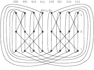
The wrapped butterfly (butterfly for short) BF_nis a graph with n2n_{vertices such that each vertex, at level i, is labeled}

by 具a0a₁. . . a_n⫺1, i典 with 0 ⱕ i ⱕ n ⫺ 1 and a_j 僆 {0,

1} for all 0 ⱕ j ⱕ n ⫺ 1. Edges of BF_nare described as

follows: Vertex 具a0a₁. . . a_i. . . a_n⫺1, i典 is adjacent to vertex 具a0a₁. . . a_i. . . a_n⫺1, (i ⫹ 1)mod n典 by a straight

edge and adjacent to vertex 具a0a₁. . . a៮_i . . . a_n⫺1, (i ⫹ 1)mod n典 by a cross edge. Figure 1 illustrates BF3.

In [5], Vadapalli and Srimani proposed a family of

degree four Cayley graphs, G_n. Later, Chen and Lau [2]

pointed out that G_n is isomorphic to BF_n. Thus, we can

combine all the results of G_nand BF_n. To prove our main result, we will describe some properties of BF_nproposed by [5]. Throughout the paper, the edges of BF_nare defined by the following four generators g, g⫺1, f, and f⫺1 in the graph:

g共具a0a1. . . an⫺1, k典兲 ⫽ 具a0a1. . . an⫺1,共k ⫹ 1兲mod n典,

f共具a0a1. . . an⫺1, k典兲

⫽ 具a0a1. . .ak⫺1a៮kak⫹1. . . an⫺1,共k ⫹ 1兲mod n典, g⫺1共具a0a1. . . an⫺1, k典兲

⫽ 具a0a1. . . an⫺1,共k ⫺ 1兲mod n典, and

f⫺1共具a0a1. . . an⫺1, k典兲

⫽ 具a0a1. . . ak⫺2a៮k⫺1ak. . . an⫺1,共k ⫺ 1兲mod n典. Hence, the g-edges, (u, g(u)) or (u, g⫺1(u)), and the

f-edges, (u, f(u)) or (u, f⫺1(u)), for some u 僆 V(BFn),

represent the straight edges and cross edges, respectively. Consequently, we have Lemma 1:

Lemma 1. f⫺1(g(u))⫽ g⫺1(f(u)) for any vertex u in BFn. 2.2. g-Cycles and g-Edges

Let u be any vertex of BF_n. We observe that gn_{(u)⫽ u.}

Moreover, 具u 3 g(u) 3 g2_{(u) 3 . . . 3 g}n_{(u)典 forms a}

simple cycle C_gu_{of length n. We call such a cycle of BF} na g-cycle at u. Hence, C_gv_{⯝ C} g u_{if and only if v僆 V(C} g u_{). As}

a result, all g-cycles form a partition of the straight edges of

BF_n. Meanwhile, any f-edge joins vertices from two differ-ent g-cycles. It can be seen that (u, f(u)) joins vertices from

C_gu_{and C} g

f(u)_{. Lemmas 2 and 3 were proved in [5].}

Lemma 2 [5]. (g(u), g⫺1(f(u))) is an f-edge joining

verti-ces of Cg u

and Cg f(u)

. Moreover, the path 具u 3 f(u) 3

g⫺1(f(u))3 g(u) 3 u典 forms a cycle of length 4.

Any Cg

u

contains exactly one vertex at each level. In particular, Cg

u

contains exactly one vertex at level 0, say 具a0a1. . . an⫺1, 0典. We use Cg

(a0a1. . .an⫺1)

as the name for

Cg u

. Now, we form a new graph BFn

G

with all the g-cycles of BFnas vertices, where two different g-cycles are joined

with an edge if and only if there exists at least one f-edge

TABLE 1. Summarizing all the results about faulty edges and/or vertices in BFn where the star (*) symbol denotes that the result is

optimal. Faulty set Hwang and Chen [3] Vadapalli and

Srimani [6] Our result

n is odd 1 edge and 1 vertex n2n_{⫺ 1*}

2 edges n2n_*

2 vertices n2n_{⫺ 4 n2}n_{⫺ 2*}

n is even 1 edge and 1 vertex n2n_{⫺ 2*}

2 edges n2n_*

2 vertices n2n_{⫺ 4*}

joining them. The vertex of BFn G corresponding to Cg u is denoted by C៮g u

. We recall the definition of the hypercube as follows: An dimensional hypercube (abbreviated to an n-cube) consists of 2n vertices which are labeled with the 2n binary numbers from 0 to 2n⫺ 1. Two vertices are connected by an edge if and only if their labels differ by exactly one bit.

Lemma 3 [5]. BFn G

is isomorphic to an n-dimensional hypercube. Moreover, the set of vertices which are adjacent to C៮g (a0a1. . .an⫺1)_{is {C}៮ g (a៮0a1. . .an⫺1)_{, . . . , C}៮ g (a0a1. . .a៮n⫺1)_}. Let h ⫽ (C៮g u , C៮gv) be any edge of BFn G . We use X(h) to denote the set of edges in BFnjoining vertices from Cg

u

and

Cgv. Using standard counting techniques, we have the

fol-lowing two corollaries:

Corollary 1 [3]. If (u, f(u))僆 X(h), then (g(u), f⫺1(g(u))) 僆 X(h) and 兩X(h)兩 ⫽ 2.

Corollary 2 [5]. There is a unique cycle C such that edges of BFnjoining vertices between Cg

u

and C are exactly (u, f(u)) and (g(u), f⫺1(g(u))), and in that case, C is isomorphic to Cg

f(u)

. According to Corollaries 1 and 2, any edge h⫽ (C៮g

u

, C៮gv)

in BFn G

induces a unique 4-cycle in BFn, with two f-edges

and two g-edges. We use Xf(Cg u

, Cgv) to denote the set of f-edges in this 4-cycle and Xg(Cg

u

, Cgv) to denote the set of g-edges in this cycle.

Lemma 4. Let T be any subtree of BFn G and let Cg T be the subgraph of BFngenerated by

冉

艛

艛

冊

艛

Proof. Let T be a subtree of BFn G

and let (C៮g u

, C៮gv) be

an edge of T. Hence, two cycles Cg

u

and Cgv in BFn are

joined by two f-edges Xf(Cg u

, Cgv). It is easy to see that E(Cg u )艛 E(Cgv)艛 Xf(Cg u , Cgv)⫺ Xg(Cg u , Cgv) forms a cycle

of length 2n in BFn. Therefore, the cycle Cg T of BFncan be generated by

冉

艛

艛

冊

艛

At the same time, the length of Cg T

is n ⫻ 兩V(T)兩. ■

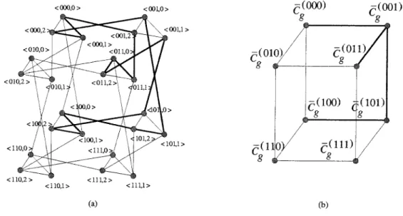
In Figure 2(a), we have another layout of BF3. The graph

BF3

G

is shown in Figure 2(b). For example, Xf(Cg

(000) , Cg (001) ) ⫽ {(具000, 0典, 具001, 2典), (具000, 2典, 具001, 0典)} and Xg(Cg (000) , Cg (001) ) ⫽ {(具000, 0典, 具000, 2典), (具001,

0典, 具001, 2典)}. Let T be the tree indicated by bold lines in Figure 2(b). The corresponding Cg

T

is indicated by bold lines in Figure 2(a).

2.3. f-Cycles and f-Edges

Let u⫽ 具a0a1. . . an⫺1, k典 be any vertex of BFnand let u˜ denote the vertex 具a៮0a៮1. . . a៮n⫺1, k典. One can see that

fn(u) ⫽ u˜ and f2n(u) ⫽ u. Moreover, 具u 3 f(u) 3

f2(u)3 . . . 3 f2n(u)典 forms a simple cycle of length 2n, denoted by Cf

u

. So, all f-cycles form a partition of the cross

edges of BFn. Meanwhile, any g-edge joins vertices from

two different f-cycles. Also, then, (u, g(u)) joins vertices from Cf

u

and Cf g(u)

. Lemmas 5 and 6 were proved in [5].

Lemma 5 [5]. (f(u), g⫺1(f(u))), (u˜, g(u˜)), (f(u˜), g⫺1(f(u˜)))

are g-edges joining vertices of Cf u

and Cf g(u)

. Moreover, the

paths具u 3 f(u) 3 g⫺1(f(u))3 g(u) 3 u典 and 具u˜ 3 f(u˜) 3

g⫺1(f(u˜))3 g(u˜) 3 u˜典 form two 4-cycles in BFn.

Any Cf

u

contains exactly two vertices at each level. Suppose that u is one of the vertices in Cf

u

at level i. Then, the other vertex in Cf

u

at level i is u˜. Thus, Cf u

contains exactly one vertex at level 0, say具a0a1. . . an⫺1, 0典, with

an⫺1⫽ 0. We use Cf

(a0a1. . .an⫺20)_{as the name for C}

f u

. Now,

we form a new graph BFn

F

with all the f-cycles of BFnas

vertices, where two different f-cycles are joined with an edge if and only if there exists a g-edge joining them. The vertex of BFn F corresponding to Cf u is denoted by C៮f u . We recall the definition of the folded hypercube as follows: An

n-dimensional folded hypercube is basically an n-cube

aug-mented with 2n⫺1 complement edges. Each complement

edge connects two vertices whose labels are complements to each other.

Lemma 6 [5]. BFn F

is isomorphic to the (n ⫺ 1)-dimen-sional folded hypercube. Moreover, the set of vertices which are adjacent to C៮f (a0a1. . .an⫺20) is {C៮f (a៮0a1. . .an⫺20) , C៮f (a0a៮1. . .an⫺20) , . . . , C៮f (a0a1. . .a៮n⫺20) }艛 {C៮f (a៮0a៮1. . .a៮n⫺20) }. Let h ⫽ (C៮f u , C៮fv) be any edge of BFn F . We use Y(h) to denote the set of edges of BFnjoining vertices from Cf

u

and

Cfv. Using standard counting techniques, we have the

fol-lowing two corollaries:

Corollary 3 [3]. If (u, g(u))僆 Y(h), then (f(u), g⫺1(f(u))), (u˜, g(u˜)), and (f(u˜), g⫺1(f(u˜))) are in Y(h) and 兩Y(h)兩 ⫽ 4.

Moreover, {u, f(u), g(u), g⫺1(f(u))} and {u˜, f(u˜), g(u˜),

g⫺1(f(u˜))} induce two 4-cycles in BF_n.

Corollary 4 [5]. There is a unique cycle C such that edges of BFn joining vertices between Cf

u

and C are exactly (u, g(u)), (f(u), g⫺1(f(u))), (u˜, g(u˜)), and (f(u˜), g⫺1(f(u˜))), and in

that case, C is isomorphic to Cf g(u)

.

According to Corollaries 3 and 4, any edge h⫽ (C៮fu, C៮fv)

induces two 4-cycles in BFn. Let ␣ be an assignment of

(C៮fu, C៮fv) 僆 E(BFnF) such that ␣(h) is the subset of Y(h)

induced by the 4-cycles of BFn. We use Yf␣(Cfu, Cfv) to

denote the set of f-edges induced by␣(h) and Yg␣(Cfu, Cfv)

to denote the set of g-edges induced by ␣(h). Hence,

兩Yf␣(Cfu, Cfv)兩 ⫽ 兩Yg␣(Cfu, Cfv)兩 ⫽ 2.

Lemma 7. Let T be any subtree of BFn F and let Cf T,␣_{be the} subgraph of BFngenerated by

冉

艛

艛

冊

艛

Then, CfT,␣is a cycle of BFnof length 2n⫻ 兩V(T)兩.

Proof. Let T be a subtree of BFn F and let (C៮f u , C៮fv) be an edge of T. Hence, (C៮f u

, C៮fv) induces two 4-cycles in BFn.

Let ␣ be an assignment of (C៮f u , C៮fv) 僆 E(BFn F ) such that ␣((C៮f u

, C៮fv)) induced a 4-cycles in BFn. Consequently, two

cycles Cf u

and Cfvare joined by two g-edges in Yg␣(Cf u

, Cfv).

It is easy to see that E(Cf

u ) 艛 E(Cfv) 艛 Yg␣(Cf u , Cfv) ⫺ Yf␣(Cf u

, Cfv) forms a cycle of length 4n in BFn.

There-fore, the subgraph Cf

T,␣_{of BF} n generated by

冉

艛

艛

冊

艛

is a cycle. Moreover, the length of Cf

T,␣_{is 2n ⫻ 兩V(T)兩.}

■

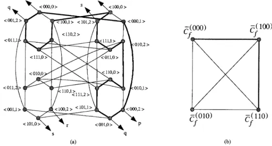
In Figure 3(a), we have another layout of BF3. The graph

BF3

F

is shown in Figure 3(b). For example, Yg␣(Cf

(000) , Cf (100) ) ⫽ {(具000, 0典, 具000, 1典), (具100, 0典, 具100, 1典)} and Yf␣(Cf (000) , Cf (100) ) ⫽ {(具000, 0典, 具100, 1典), (具100,

0典, 具000, 1典)}. Let T be the tree indicated by bold lines in

Figure 3(b). The corresponding Cf

T,␣ _{is indicated by bold} lines in Figure 3(a).

3. CYCLE EMBEDDING IN A FAULTY WRAPPED BUTTERFLY GRAPH

Let F denote a faulty set in a wrapped butterfly graph

BFnand assume that F has at most two elements. Then, we

will determine the maximum length of a cycle in the graph

BFn⫺ F. In [3], Hwang and Chen showed that the length

of the cycle is n2n when F consists of two edges.

Lemma 8 [3]. For any integer nⱖ 3, BF_n⫺ F is Ham-iltonian if F consists of two edges.

On the other hand, Vadapalli and Srimani [6] proposed the following lemma when a wrapped butterfly graph does not have any edge fault but has at most two vertex faults:

Lemma 9 [6]. For any integer nⱖ 3, BFn⫺ F contains a cycle of length n2n_{⫺ 2 if F consists of one vertex and a} cycle of length n2n_{⫺ 4 if F consists of two vertices.}

In the remaining part of this section, we propose three

can be embedded in BFn ⫺ F for any n ⱖ 3 when F

consists of one vertex and one edge. Lemma 11 shows that

the maximum cycle length is n2n _{⫺ 1 if n is odd when F}

consists of one vertex and one edge. Lemma 12 verifies that

the maximum cycle length is n2n_{⫺ 2 for odd n ⱖ 3 when}

F consists of two vertices. To prove these three lemmas, we

use three fundamental cycles, denoted by Ꮾ1, Ꮾ2, and

Ꮾ3( j), respectively, to construct a larger cycle in a faulty wrapped butterfly graph.

The cycleᏮ1shown in Figure 4(a) is constructed as

follows: Let a1 ⫽ 具00. . .0

n

, 1典 and P1 be the path具a13

g(a1) 3 g 2 (a1) 3 . . . 3 g n⫺2_(a 1)典. Hence, g n⫺2_共a1兲 ⫽ a2 ⫽ 具00. . .0 n , n ⫺ 1典, f共a2兲 ⫽ 具00. . .0 n⫺1 1, 0典 ⫽ a3, and f共a3兲 ⫽ 具1 00. . .0 n⫺2

1, 1典 ⫽ a4. Let P2be the path具a4

3 g(a4) 3 g2(a4) 3 . . . 3 g n⫺1_(a 4)典. Consequently, gn⫺1_{共a4兲 ⫽ a5⫽ 具1 00. . .0} n⫺2 1, 0典 and f⫺1共a5兲 ⫽ 具1 00. . .0 n⫺1 ,

n ⫺ 1典 ⫽ a6. Let P3 be the path 具a6 3 g⫺1(a6) 3

g⫺2(a6) 3 . . . 3 g⫺(n⫺1)(a6)典. Thus, g⫺共n⫺1兲共a6兲 ⫽ a7 ⫽ 具1 00. . .0

n⫺1

, 0典 and f(a7)⫽ a1. LetᏮ1be具a13 P13

a2 3 a3 3 a4 3 P2 3 a5 3 a6 3 P3 3 a73 a1典. Obviously, P1is a path in Cg a1_{, P} 2is a path in Cg a4_{, and P} 3 is a path in Cg a6_{. Since V(C} g u ) 艚 V(Cgv) ⫽ A for u ⫽ v 僆

{a1, a4, a6} and nⱖ 3, P1, P2, and P3are disjoint paths. Therefore,Ꮾ1is a cycle of length 3n.

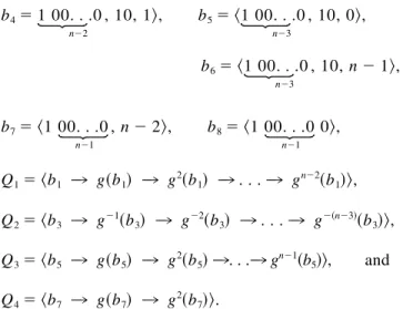
Similarly, we can construct the basic cycleᏮ2shown in Figure 4(b) as follows: Let Ꮾ2 ⫽ 具b1 3 Q1 3 b2 3 b3 3 Q2 3 b4 3 b5 3 Q33 b6 3 b7 3 Q43 b8 3 b1典, where b1⫽ 具00. . .0 n , 1典, b2⫽ 具00. . .0 n , n⫺ 1典, b3 ⫽ 具00. . .0 n⫺2 , 10, n⫺ 2典,

FIG. 3. (a) Another layout of BF3; (b) the graph BF3

F_.

FIG. 4. (a) A cycleᏮ1of length 3n if nⱖ 3; (b) a cycle Ꮾ2of length 3n if nⱖ 3; (c) a cycle Ꮾ3( j) of length

b4⫽ 1 00. . .0 n⫺2 , 10, 1典, b5⫽ 具1 00. . .0 n⫺3 , 10, 0典, b6⫽ 具1 00. . .0 n⫺3 , 10, n⫺ 1典, b7⫽ 具1 00. . .0 n⫺1 , n⫺ 2典, b8⫽ 具1 00. . .0 n⫺1 0典, Q1⫽ 具b1 3 g共b1兲 3 g 2_{共b1兲 3 . . . 3 g}n⫺2_共b1兲典, Q2⫽ 具b3 3 g⫺1共b3兲 3 g⫺2共b3兲 3 . . . 3 g⫺共n⫺3兲共b3兲典, Q3⫽ 具b5 3 g共b5兲 3 g 2 共b5兲 3. . .3 g n⫺1_共b 5兲典, and Q4⫽ 具b7 3 g共b7兲 3 g 2 共b7兲典. Q1is a path in Cg b1_{, Q} 2is a path in Cg b3_{, Q} 3is a path in Cg b5_{, and Q} 4is a path in Cg b7_{. Since V(C} g u ) 艚 V(Cg v ) ⫽ A

for u ⫽ v 僆 {b1, b3, b5, b7} and nⱖ 3, Q1, Q2, Q3, and

Q4are disjoint paths. Consequently,Ꮾ2is a cycle of length 3n.

Fix some j with 2ⱕ j ⱕ n ⫺ 1. The cycle Ꮾ3( j) shown

in Figure 4(c) is constructed as follows:

Let Ꮾ3( j) ⫽ 具c1 3 R1 3 c2 3 c3 3 R2 3 c4 3 c5 3 R3 3 c6 3 c73 R4 3 c8 3 c1典, where c1⫽ 具00. . .0 n , 1典, c2⫽ 具00. . .0 n , j⫺ 1典, c3⫽ 具00. . .0 j⫺1 , 1 00. . .0 n⫺j , j典, c4⫽ 具00. . .0 j⫺1 1 00. . .0 n⫺j , 0典, c5⫽ 具1 00. . .0 j⫺2 1 00. . .0 n⫺j , 1典, c6⫽ 具1 00. . .0 j⫺2 1 00. . .0 n⫺j , j典, c7⫽ 具1 00. . .0 n⫺1 , j⫺ 1典, c8⫽ 具1 00. . .0 n⫺1 , 0典, R1⫽ 具c1 3 g共c1兲 3 g 2 共c1兲 3 . . . 3 g j⫺2_共c 1兲典, R2⫽ 具c3 3 g⫺1共c3兲 3 g⫺2共c3兲 3 . . . 3 g⫺j共c3兲典, R3⫽ 具c5 3 g⫺1共c5兲 3 g⫺2共c5兲 3 . . . 3 g⫺共n⫺j⫹1兲共c5兲典, and R4⫽ 具c7 3 g⫺1共c7兲 3 g⫺2共c7兲 3 . . . 3 g⫺共n⫺j⫹1兲共c7兲典. R1 is a path in Cg c1_{, R} 2is a path in Cg c3_{, R} 3is a path in Cg c5_{, and C} 4is a path in Cg c7_{. Since V(C} g u )艚 V(Cg v )⫽ A for u ⫽ v 僆 {c1, c3, c5, c7} and n ⱖ 3, R1, R2, R3, and R4

are disjoint paths. Consequently,Ꮾ3( j) is a cycle of length

2n ⫹ 4. We even have b3⫽ b4 and c1⫽ c2 if and only

if n ⫽ 3. We have V(Ꮾl) 艚 V(Ꮾk) ⫽ A for 1 ⱕ l ⫽ k

ⱕ 3 and n ⱖ 4 because P1⫽ Q1and P1 艚 R1⫽ A.

Lemma 10. For any integer n ⱖ 3, BFn⫺ F contains a cycle of length n2n⫺ 2 if F consists of one vertex and one edge.

Proof. Since BFn is vertex transitive, we assume that

the faulty vertex is x⫽ 具00 . . . 0, 0典 and the faulty edge is e.

CASE 1. e is a g-edge: Let e ⫽ (u, g(u)) for some u

僆 V(BFn). Since n ⱖ 3 and BFn

F

is isomorphic to an (n

⫺ 1)-dimensional folded hypercube, BFn

F _{⫺ {C៮} f x , (C៮f u , C៮f g(u)

)} is connected. Let T be any spanning tree of BFn F_⫺ {C៮f x , (C៮f u , C៮f g(u) )}. By Lemma 7, Cf

T,␣_{for any␣ forms an}

n2n⫺ 2n cycle. Let Sg⫽ {( y, g( y))兩y ⫽ f

2k

( x); 1 ⱕ k

ⱕ n ⫺ 1}, S⬘g ⫽ {( f( y), g⫺1( f( y)))兩y ⫽ f

2k

( x); 1 ⱕ k

ⱕ n ⫺ 1}, Sf⫽ {( y, f( y))兩y ⫽ f

2k

( x); 1 ⱕ k ⱕ n ⫺ 1},

and S⬘f ⫽ {( g( y), f⫺1( g( y)))兩y ⫽ f

2k ( x); 1 ⱕ k ⱕ n ⫺ 1}. Accordingly, Sf 傺 E(Cf x ) and S⬘f 傺 E(Cf g( x) ). CASE1.1. eⰻ S_g艛 S⬘_g(see Fig. 5): One can observe that

Sg艛 S⬘g艛 Sf艛 S⬘fforms n ⫺ 1 disjoint 4-cycles in BFn.

Meanwhile, S⬘f傺 E(CfT,␣) and Sf艚 E(CfT,␣)⫽ A. Hence,

共E共Cf T,␣_{兲 艛 S}

g艛 S⬘g艛 Sf兲 ⫺ S⬘f

forms a cycle in BFn⫺ F and the cycle length is n2n⫺ 2.

CASE 1.2. e 僆 S_g艛 S⬘_g: Constructing the cycle of length

n2n ⫺ 2 is similar to Case 1.1 except that Sg ⫽ {( y,

g( y))兩y ⫽ f2k⫺1( x); 1 ⱕ k ⱕ n ⫺ 1}, S⬘g ⫽ {( f( y), g⫺1( f( y)))兩y ⫽ f2k⫺1( x); 1 ⱕ k ⱕ n ⫺ 1}, Sf ⫽ {( y, f( y))兩y ⫽ f2k⫺1( x); 1 ⱕ k ⱕ n ⫺ 1}, and S⬘f ⫽ {( g( y), f⫺1( g( y)))兩y ⫽ f2k⫺1( x); 1 ⱕ k ⱕ n ⫺ 1}.

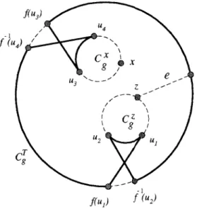
FIG. 5. An illustration for Case 1.1 with n⫽ 3, Sg⫽ {(u2, g(u2)), (u4,

g(u4))}, S⬘g ⫽ {(u3, g⫺1(u3)), (u5, g⫺1(u5))}, Sf⫽ {(u2, u3), (u4,

CASE 2. e is an f-edge: Let e ⫽ (u, f(u)) for some u

僆 V(BFn).

CASE 2.1. n is an even integer: Since n ⱖ 3 and BF_nG is

isomorphic to the n-dimensional hypercube, BFn

G _{⫺ {C៮} g x , (C៮g u , C៮g f(u)

)} is connected. Let T be any spanning tree of

BFn G_{⫺ {C៮} g x , (C៮g u , C៮g f(u) )}. By Lemma 4, Cg T forms a cycle spanning V(BFn) ⫺ V(Cg x

). Since T does not contain the edge (C៮g u , C៮g f(u) ) and e 僆 Xf(Cg u , Cg f(u) ), Cg T does not

contain the faulty edge e. Let S ⫽ {Xf(Cg

y , Cg f( y) )兩y ⫽ g2k ( x); 1 ⱕ k ⬍ n/ 2}.

CASE2.1.1. e ⰻ S: One can observe that 艛(u,v)_僆SX_g(C_gu,

Cgv) 艛 S forms (n/ 2) ⫺ 1 disjoint 4-cycles in BFn⫺ F.

Let S1⫽ {( f( y), g⫺1( f( y)))兩y ⫽ g 2k ( x); 1ⱕ k ⬍ n/ 2}. Hence, S1 傺 E(Cg T ) and S1 傺 艛(u,v)僆S Xg(Cg u , Cgv). Therefore,

艛

forms a cycle of length n2n⫺ 2 in BFn⫺ F.

CASE2.1.2. e僆 S: The cycle can be constructed using the

method of Case 2.1.1 except that S ⫽ {Xf(Cgy, Cgf( y))兩y

⫽ g2k⫺1_{( x); 1 ⱕ k ⬍ n/ 2}.}

CASE 2.2. n is an odd integer: Let S₁ ⫽ {X_f(C_gy, C_gf( y))兩y

⫽ g2k⫺1_{( x); 1 ⱕ k ⱕ (n ⫺ 1)/ 2}.}

CASE2.2.1. eⰻ S1(see Fig. 6): Since C៮_gu⫽ C៮_gf(u), we can

choose z 僆 {u, f(u)} according to the following rules:

(1) If either C៮g u_{⫽ C៮} g x or C៮gf(u)⫽ C៮g x

, then we choose z such that C៮g

z

⫽ C៮g x

.

(2) Otherwise, we choose z such that (C៮g z , C៮g x )ⰻ E(BFn G ). Since n ⱖ 3 and BFn G is isomorphic to an n-dimensional hypercube, BFn G _{⫺ {C៮} g x , C៮g z

} is connected. Let T be any spanning tree of BFn G _{⫺ {C៮} g x , C៮g z }. By Lemma 4, Cg T is a cycle spanning V(BFn) ⫺ V(Cg x ) ⫺ V(Cg z

) and it does not contain e. Let S2⫽ {Xf(Cg

y

, Cg f( y)

)兩y ⫽ g2k⫺1( z); 1 ⱕ k

ⱕ (n ⫺ 1)/ 2}. Hence, S1艚 S2⫽ A, and S1艛 S2is fault

free. We observe that艛(u,v)_僆S

1Xg(Cg

u

, Cgv) 艛 S1forms (n

⫺ 1)/ 2 disjoint 4-cycles and 艛(u,v)僆S2 Xg(Cg

u

, Cgv) 艛 S2

forms (n ⫺ 1)/ 2 disjoint 4-cycles. Let S3 ⫽ {( f( y),

g⫺1( f( y)))兩y ⫽ g2k⫺1( x); 1 ⱕ k ⱕ (n ⫺ 1)/ 2} and S4 ⫽ {( f( y), g⫺1_{( f( y)))兩y ⫽ g}2k⫺1_{( z); 1 ⱕ k ⱕ (n ⫺ 1)/}

2}. Hence, S3 艚 S4 ⫽ A and S3 艛 S4 傺 E(Cg

T ). Meanwhile, S3艛 S4傺 艛(u,v)僆(S1艛S2)Xg(Cg u , Cgv). There-fore,

艛

forms a cycle in BFn⫺ F and this cycle length is n2 n_{⫺ 2.}

CASE2.2.2. e 僆 S1(see Fig. 7): Since nⱖ 3, there exists

y 僆 V(BFn) such that f( y) 僆 V(Cg

x

). So, both ( y, f( y)) and ( g( y), f⫺1( g( y))) join vertices of Cg

y and Cg x . Let W1 ⫽ V(Cg a1₎艛 V(C g a3₎艛 V(C g a5₎艛 V(C g a7_{) and W}៮ 1⫽ {C៮g a1_, C៮g a3_{, C}៮ g a5_{, C}៮ g a7_{}. Hence, C}៮ g y

is not adjacent to any vertex in

W៮1 ⫺ {C៮g x }. Since n ⱖ 3 and BFn G is isomorphic to an n-dimensional hypercube, BFn G _{⫺ W៮1 ⫺ {C៮} g y } is con-nected. Let T be any spanning tree of BFn

G_{⫺ W៮1⫺ {C៮} g y }. By Lemma 4, Cg T is a cycle spanning V(BFn) ⫺ W1 ⫺ V(Cg y

). There exists w僆 V(Ꮾ1) such that Xf(Cg w

, Cg f(w)

) is fault free and (w, f(w)) joins some vertex in bothᏮ1and

Cg T . Then, Ce⫽ 共E共Ꮾ1兲 艛 E共Cg T 兲 艛 Xf共Cg w , Cg f共w兲_{兲兲 ⫺ X} g共Cg w , Cg f共w兲_兲

forms a cycle of length n2n⫺ 2n spanning (V(BFn)⫺ W1

⫺ V(Cg y )) 艛 V(Ꮾ1). Let S3 ⫽ {Xf(Cg s , Cg f(s) )兩s ⫽ g2k⫺1(a3); 1 ⱕ k ⱕ (n ⫺ 1)/ 2} and S4 ⫽ {Xf(Cg t , Cg f(t) )兩t ⫽ g2k⫺1( y); 1 ⱕ k

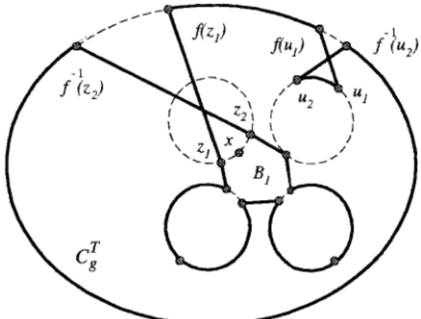
FIG. 6. An illustration for the Case 2.2.1 with n⫽ 3, S1⫽ {(u3, f(u3)),

(u4, f⫺1(u4))} and S2⫽ {(u1, f(u1)), (u2, f⫺1(u2))}.

FIG. 7. An illustration for the Case 2.2.2 with n⫽ 3, S3⫽ {(u3, f(u3)),

ⱕ (n ⫺ 1)/ 2}. Hence, S3艚 S4⫽ A and S3艛 S4is fault free. We observe that艛_{(u,v)僆(S3艛S4})Xg(Cg

u

, Cg v

))艛 S3艛

S4 forms n ⫺ 1 disjoint 4-cycles. Let S5 ⫽ {( f(s),

g⫺1( f(s)))兩s ⫽ g2k⫺1(a3); 1 ⱕ k ⱕ (n ⫺ 1)/ 2} and S6 ⫽ {( f(t), g⫺1_{( f(t)))兩t ⫽ g}2k⫺1_{( y); 1ⱕ k ⱕ (n ⫺ 1)/ 2}.} Hence, S5艚 S6⫽ A and S5艛 S6is a subset of both E(Ce)

and 艛(u,v)僆(S_3艛S4)Xg(Cg u , Cg v )). Therefore,

艛

forms a cycle of length n2n⫺ 2 in BFn⫺ F. ■

Lemma 11. For any odd integer n ⱖ 3, BFn ⫺ F is Hamiltonian if F consists of one vertex and one edge.

Proof. Since BFnis vertex transitive, we may assume

that the faulty vertex is x ⫽ 具00 . . . 0, 0典 and the faulty edge is e. Let W1⫽ V(Cga1)艛 V(Cga3)艛 V(Cga5)艛 V(Cga7)

and W៮1 ⫽ {C៮ga1, C៮ga3, C៮ga5, C៮ga7}.

CASE 1. e is an f-edge: Let e ⫽ (u, f(u)) for some u

僆 V(BFn).

CASE1.1. {u, f(u)} 艚 (V(C_ga3₎艛 V(C

g

a7₎₎⫽ A (see Fig.

8): Since nⱖ 3 and BFnGis isomorphic to an n-dimensional

hypercube, BFnG ⫺ W៮1 ⫺ {(C៮gu, C៮gf(u))} is connected. Let T be any spanning tree of BFnG⫺ W៮1⫺ {(C៮gu, C៮gf(u))}. By

Lemma 4, CgTis a cycle spanning V(BFn)⫺ W1and it does

not contain e.

Let S ⫽ {Xf(Cgy, Cgf( y))兩y ⫽ g2k⫺1(a3); 1 ⱕ k ⱕ (n ⫺ 1)/ 2}. Hence, 艛(u,v)僆S Xg(Cgu, Cgv) 艛 S forms (n

⫺ 1)/ 2 disjoint 4-cycles. Let S1⫽ {( f( y), g⫺1_{( f( y)))兩y} ⫽ g2k⫺1_(a

3); 1 ⱕ k ⱕ (n ⫺ 1)/ 2}. Consequently, S1is

a subset of both 艛(u,v)_僆S Xg(Cgu, Cgv) and E(CgT).

There-fore, Ce⫽

艛

forms a cycle of length n2n ⫺ 3n ⫺ 1 spanning V(BFn)

⫺ V(Ꮾ1)⫺ { x} and it does not contain e. Since the length ofᏮ1is 3n, there exists z僆 V(Ꮾ1) such that Xf(Cg

z

, Cg f( z)

) is fault free and ( z, f( z)) joins some vertex in both Ceand

Ꮾ1. Therefore, 共E共Ce兲 艛 E共Ꮾ1兲 艛 Xf共Cg z , Cg f共 z兲_{兲兲 ⫺ X} g共Cg z , Cg f共 z兲_兲

forms a Hamiltonian cycle of BFn ⫺ F.

CASE1.2. {u, f(u)} 艚 (V(C_ga3₎艛 V(C

g a7₎₎⫽ A (see Fig. 9): Let S ⫽ {Xf(Cg y , Cg f( y) )兩y ⫽ g2k⫺1( x); 1 ⱕ k ⱕ (n

⫺ 1)/ 2}. Hence, e ⰻ S. Since n ⱖ 3 and BFn

G

is

isomorphic to an n-dimensional hypercube, BFn

G_{⫺ {C៮}

g x

} is connected. Let T be any spanning tree of BFn

G_{⫺ {C៮} g x }. By Lemma 4, Cg T is a cycle spanning V(BFn) ⫺ V(Cg x ). Since

S is fault free,艛(u,v)_僆SXg(Cg u

, Cg v

)艛 S forms (n ⫺ 1)/ 2

disjoint 4-cycles. Let S1 ⫽ {( f( y), g⫺1( f( y)))兩y

⫽ g2k⫺1_{( x); 1ⱕ k ⱕ (n ⫺ 1)/ 2}. Hence, S1is a subset} of both 艛(u,v)_僆S Xg(Cg u , Cg v ) and E(Cg T ). Therefore,

艛

forms a Hamiltonian cycle of BFn ⫺ F.

CASE 2. e is a g-edge: Let e ⫽ (u, g(u)) for some u

僆 V(BFn).

CASE 2.1. C៮_gu ⫽ C៮_gx: Since n ⱖ 3 and BF_nG is isomorphic

to an n-dimensional hypercube, BFn

G _{⫺ W៮1}

is connected.

Let T be any spanning tree of BFn

G _{⫺ W៮1}

. Constructing a Hamiltonian cycle for this case is very similar to Case 1.1 except that the chosen vertex z is vertex u when e

僆 E(Ꮾ1).

CASE 2.2. C៮_gu ⫽ C៮_gx and C៮_gu is not connected with C៮_gx in

BFn G : Since nⱖ 3 and BFn G is isomorphic to an n-dimen-sional hypercube, BFn G _{⫺ {C៮} g x } is connected. Let T be a spanning tree of BFn G _{⫺ {C៮} g x } such that (C៮g u , C៮g f(u) )

FIG. 8. An illustration for the Case 1.1 with n⫽ 3 and S ⫽ {(u1, f(u1)),

(u2, f⫺1(u2))}.

FIG. 9. An illustration for the Case 1.2 with n⫽ 3 and S ⫽ {(u1, f(u1)),

僆 E(T). Then, the Hamiltonian cycle of BFn⫺ F can be

constructed by the same method used in Case 1.2.

CASE 2.3. (C៮_gu, C៮_gx) 僆 E(BF_nG) (i.e., C៮_gu and C៮_gx are

con-nected):

CASE2.3.1. C៮_gu⫽ C៮_ga3_{and C}៮

g u_{⫽ C៮}

g

a7_{(see Fig. 10): Since n}

ⱖ 3 and BFn

G_{is isomorphic to an n-dimensional hypercube,}

BF_nG _{⫺ W៮1 ⫺ {C៮}

g

u_{} is connected. Let T be any spanning}

tree of BF_nG _{⫺ W៮1 ⫺ {C៮} g u_{}. By Lemma 4, C} g T _{is a cycle} spanning V(BF_n) ⫺ W1 ⫺ V(C_gu_{). Let S ⫽ {X} f(Cg y_, C_gf( y)_{)兩y ⫽ g}2k⫺1_(a 3); 1 ⱕ k ⱕ (n ⫺ 1)/ 2}. Hence, 艛(u,v)僆S Xg(Cg u_{, C} g v_{) 艛 S forms (n ⫺ 1)/ 2 disjoint}

4-cycles. Let S₁ ⫽ {( f( y), g⫺1( f( y)))兩y ⫽ g2k⫺1(a₃); 1

ⱕ k ⱕ (n ⫺ 1)/ 2}. Accordingly, S1 is a subset of both

艛(u,v)僆SXg(Cg u_{, C} g v_{) and E(C} g T_{). Therefore,} Ce⫽

艛

forms a cycle spanning V(BFn)⫺ V(Ꮾ1)⫺ V(Cgu)⫺ { x}.

Since the length of Ꮾ1 is 3n, we can choose a vertex z

僆 V(Cgu) such that f( z) 僆 V(Ce) if f(u)僆 V(Ꮾ1) or f( z)

僆 V(Ꮾ1) if f(u) ⰻ V(Ꮾ1). Therefore,

共E共Ce兲 艛 E共Ꮾ1兲 艛 E共Cg

u_{兲 艛 X} f共Cg u , Cg f共u兲_{兲 艛 X} f共Cg z , Cg f共 z兲_兲兲 ⫺ Xg共Cg u , Cg f共u兲_{兲 ⫺ X} g共Cg z , Cg f共 z兲_兲

forms a Hamiltonian cycle of BFn ⫺ F.

CASE 2.3.2. C៮_gu ⫽ C៮_ga3 _{(see Fig. 11): Let S} ⫽ {X

g(Cgy, Cgf( y))兩y ⫽ g2k⫺1(a3); 1 ⱕ k ⱕ (n ⫺ 1)/ 2}.

Assume that eⰻ S. Since n ⱖ 3 and BFn

G

is isomorphic

to an n-dimensional hypercube, BFn

G _{⫺ W៮1}

is connected.

Let T be any spanning tree of BFn

G _{⫺ W៮1}

. Then, the

Hamiltonian cycle of BFn ⫺ F can be constructed by the

same method used in Case 1.1.

Assume that e 僆 S. Let W2 ⫽ V(Cg

b1₎ 艛 V(C g b3₎ 艛 V(Cg b5₎艛 V(C g b7_{) and W}៮ 2⫽ {C៮g b1_{, C}៮ g b3_{, C}៮ g b5_{, C}៮ g b7_{}. Since n} ⱖ 3 and BFn G

is isomorphic to an n-dimensional hypercube,

BFn

G _{⫺ W៮2}

is connected. Let T be a spanning tree of BFn G ⫺ W៮2such that (C៮g u , C៮g f(u) )僆 E(T). By Lemma 4, Cg T is a cycle spanning V(BFn) ⫺ W2. Let S2 ⫽ {Xf(Cg

y , Cg f( y) )兩y ⫽ g2k⫺1_(b 8); 1 ⱕ k ⱕ (n ⫺ 3)/ 2}. Then, Ce⫽

冉

艛

冊

forms a cycle spanning V(BFn) ⫺ V(Ꮾ2) ⫺ { x} and it

does not contain e. Since the length ofᏮ2is 3n, there exists

w僆 V(Ꮾ2) such that (w, ( f(w)) joins some vertex in both

Ce andᏮ2. Obviously, Xf(Cg w

, Cg f(w)

) is fault free. Then, 共E共Ce兲 艛 E共Ꮾ2兲 艛 Xf共Cg w , Cg f共w兲_{兲兲 ⫺ X} g共Cg w , Cg f共w兲_兲

forms a Hamiltonian cycle of BFn ⫺ F.

CASE 2.3.3. C៮gu⫽ C៮ga7.

Suppose that e僆 Xg(Cg x

, Cg

a7_{). Hence, e}⫽ (具10 . . . 00,

0典, 具100 . . . 0, 1典). We observe that e 僆 E(Ꮾ1) and eⰻ

E(Ꮾ2). Using the same method used in the situation e僆 S

of Case 2.3.2, the Hamiltonian cycle of BFn ⫺ F can be

constructed. Suppose that e ⰻ Xg(Cg x , Cg a7_{). Since n}ⱖ 3 and BF n G is

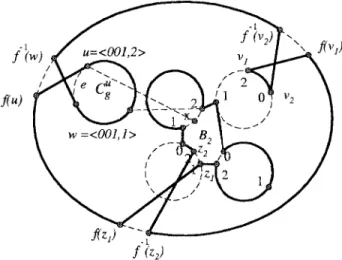
FIG. 10. An illustration for the Case 2.3.1 with n⫽ 3, S ⫽ {(v1, f(v1)),

(v2, f⫺1(v2))}, Xf(Cgu, Cgf(u)) ⫽ {(u, v3), ( z1, v4)}, Xf(Cgz, Cgf( z)))

⫽ {( z1, f( z1)), ( z2, f⫺1( z2))}, Xg(Cgu, Cgf(u))⫽ {(u, z1), (v3, v4)}, and

Xg(Cgz, Cgf( z))⫽ {( z1, z2), ( f( z1), f⫺1( z2))}.

FIG. 11. An illustration for the Case 2.3.2 with n⫽ 3, e ⫽ (具001, 2典, 具001, 1典), and S2⫽ A.

isomorphic to an n-dimensional hypercube, BFn

G _{⫺ W៮1}

is connected. Let T be any spanning tree of BFn

G_{⫺ W៮1}

and e

⫽ (u, g(u)) for some u 僆 V(BFn). Constructing a

Ham-iltonian cycle for this case is very similar to Case 1.1 except

that the chosen vertex z is vertex u when e 僆 E(Ꮾ1). ■

Lemma 12. For any odd integer n ⱖ 3, BFn ⫺ F is Hamiltonian if F consists of two vertices.

Proof. Since BFnis vertex transitive, we may assume

that one faulty vertex is x ⫽ 具00 . . . 0, 0典 and the other is

y. Let W៮3⫽ {C៮g c1_{, C}៮ g c3_{, C}៮ g c5_{, C}៮ g c7_}.

CASE 1. C៮_gx ⫽ C៮_gy (see Fig. 12): Let y ⫽ 具00. . .0

n

, j典 for

some 1 ⱕ j ⱕ n ⫺ 1. Since n is an odd integer, without

loss of generality, we may assume that j is an even integer.

Since n ⱖ 3 and BFn

G

is isomorphic to an n-dimensional hypercube, BFn

G_{⫺ W៮3}

is connected. Let T be any spanning tree of BFn G _{⫺ W៮3} . By Lemma 4, Cg T is a cycle spanning V(BFn) ⫺ W3. Let S1⫽

再

冏

冎

再

冏

冎

再

冏

冎

再

冏

冎

One can observe that Si艚 Sj⫽ A for 1 ⱕ i ⫽ j ⱕ 4 and

艛(u,v)僆S1艛S2艛S3艛S4 Xg(Cg

u

, Cg v

) 艛 S1 艛 S2 艛 S3 艛 S4

forms n ⫺ 3 disjoint 4-cycles. Let

S5⫽

再

冏

冎

再

冏

冎

再

冏

冎

再

冏

冎

S7艛 S8is a subset of both E(Cg T ) and艛(u,v)_僆S 1艛S2艛S3艛S4 Xg(Cg u , Cgv). Therefore, Ce⫽

艛

forms a cycle of length n2n ⫺ 2n ⫺ 6 spanning V(BFn)

⫺ V(Ꮾ3( j)) ⫺ { x, y}. Since the length of Ꮾ3( j) is 2n

⫹ 4, there exists z 僆 V(Ꮾ3( j)) such that Xf(Cg z

, Cg f( z)

) is fault free and ( z, f( z)) joins some vertex in both Ce and

Ꮾ3( j). Then, 共E共Ce兲 艛 E共Ꮾ3共 j兲兲 艛 Xf共Cg z , Cg f共 z兲_{兲兲 ⫺ X} g共Cg z , Cg f共 z兲_兲

forms a Hamiltonian cycle of BFn ⫺ F.

CASE2. C៮_gx ⫽ C៮_gy and C៮_gx is not connected with C៮_gy in BF_nG

(See Fig. 13): Since n ⱖ 3 and BFn

G is isomorphic to an n-dimensional hypercube, BFn G_{⫺ {C៮} g x , C៮g y } is connected. Let T be any spanning tree of BFn

G_{⫺ {C៮} g x , C៮g y }. By Lemma 4, Cg T is a cycle spanning V(BFn)⫺ V(Cg x ) ⫺ V(Cg y ). Let S1⫽ {Xf(Cg s , Cg f(s) )兩s ⫽ g2k⫺1( x); 1ⱕ k ⱕ (n ⫺ 1)/ 2} and S2 ⫽ {Xf(Cg t , Cg f(t) )兩t ⫽ g2k⫺1( y); 1 ⱕ k ⱕ (n

⫺ 1)/ 2}. Since S1艚 S2 ⫽ A and S1艛 S2 is fault free,

艛(u,v)僆S1艛S2Xg(Cg u , Cgv)艛 S1艛 S2forms n ⫺ 1 disjoint 4-cycles. Let S3 ⫽ {( f(s), g⫺1( f(s)))兩s ⫽ g 2k⫺1_{( x); 1} ⱕ k ⱕ (n ⫺ 1)/ 2} and S4 ⫽ {( f(t), g⫺1_{( f(t)))兩t} ⫽ g2k⫺1_{( y); 1 ⱕ k ⱕ (n ⫺ 1)/ 2}. Hence, S3艚 S4⫽ A} and S3 艛 S4 傺 E(Cg T

). At the same time, S3 艛 S4 傺

艛(u,v)僆(S1艛S2)Xg(Cg u , Cgv). Therefore,

艛

f(u1)), (u2, f⫺1(u2))}, S2⫽ {(u3, f(u3)), (u4, f⫺1(u4))}, S3⫽ {(u5,

forms a Hamiltonian cycle of BFn ⫺ F.

CASE 3. (C៮_gx, C៮_gy) 僆 E(BF_nG) (i.e., C៮_gx and C៮_gy are

con-nected):

CASE3.1. C៮_gy ⫽ C៮_ga3_{and C}៮

g y_{⫽ C៮}

g

a7_{(see Fig. 7): Since BF}

n G

is an n-dimensional hypercube with n ⱖ 3, Cga3, Cga5, and Cga7 are fault free. As a result, C៮ga3is not adjacent to C៮gy in BFnG. Since BFnG⫺ W៮1⫺ {C៮gy} is connected, let T be any

spanning tree of BFnG ⫺ W៮1 ⫺ {C៮gy}. The Hamiltonian

cycle of the graph BFn⫺ F can be constructed by the same

method used in Case 2.2.2 of Lemma 10.

CASE 3.2. C៮_gy ⫽ C៮_ga3 _{or C}៮ g y _⫽ C៮g a7_{: Let} S1⫽{具00. . .0 n 1, 2k ⫺ 1典兩1ⱕkⱕ(n⫺1)/ 2} and S2 ⫽ 兵具1 00. . .0 n⫺1 , 2k典兩1 ⱕ k ⱕ 共n ⫺ 1兲/ 2}. Therefore, there does not exist any edge in Xf(Cgu, Cgf(u)) which joins vertices

of Cgx and Cgy for all u僆 S1 艛 S2.

CASE3.2.1. y ⰻ S1艛 S2(See Fig. 13): Since n ⱖ 3 and

BFn G

is isomorphic to an n-dimensional hypercube, BFn

G_⫺

{C៮g x

, C៮g y

} is connected. Let T be any spanning tree of BFn G

⫺ {C៮g x

, C៮g y

}. With the same method used in Case 2, the

Hamiltonian cycle of the graph BFn ⫺ F can be

con-structed.

CASE 3.2.2. y 僆 S1 艛 S2:

Given an integer k with 0ⱕ k ⬍ n, the mapping␴kfrom V(BFn) into V(BFn) can be defined by␴k(具a0a1. . . an⫺1, l典) ⫽ 具akak⫹1. . . an⫺1a0a1. . . ak⫺1, (l ⫺ k)mod n典.

Similarly, we can define the mapping␸ifrom V(BFn) into V(BFn) as ␸i(具a0a1. . . , aiai⫹1, . . . , an⫺1, l典)

⫽ 具a0a1. . . a៮iai⫹1. . . an⫺1, l典, where 0 ⱕ i ⬍ n. Hence,

␴k and␸iare two automorphisms of BFn.

Suppose that y 僆 S1. Then, y⫽ 具00. . .0

n⫺1

1, l典 for some

odd l, 1 ⱕ l ⱕ n ⫺ 2. Accordingly, ␸n⫺1⫺l ⴰ ␴l is an

automorphism of BFn such that␸n⫺1⫺l ⴰ ␴l( y) ⫽ x and

␾n⫺1⫺lⴰ␴l共 x兲 ⫽ 00. . .0 n⫺1⫺L

1 00. . .0

l

, n⫺ l典 ⫽ z.

Conse-quently, z ⰻ S1 艛 S2. Therefore, we can construct a

Hamiltonian cycle C in BFn⫺ { x, z} by using the same

method as in Case 3.2.1. Finally, (␸n⫺1⫺lⴰ ␴l)⫺1(C) also

forms a Hamiltonian cycle of BFn ⫺ { x, y}.

Suppose that y僆 S2. Then, y⫽ 具1 00. . .0

n⫺1

, l典 for some

even l, 2 ⱕ l ⱕ n ⫺ 1. Hence,␸n⫺1ⴰ ␴lis an

automor-phism of BFn such that ␸n⫺1 ⴰ ␴l( y) ⫽ x and

␸n⫺lⴰ␴l共 x兲 ⫽ 具00. . .0 n⫺1

1典 1 00. . .0

l⫺1

, n⫺ l典 ⫽ z.

Con-sequently, z ⰻ S1 艛 S2. With the same method used in

Case 3.2.1, we can construct a Hamiltonian cycle C in BFn

⫺ { x, z}. Hence, (␸n⫺l ⴰ ␴l)⫺1(C) also forms a

Hamil-tonian cycle of BFn ⫺ { x, y}. ■

Combining Lemmas 8 –12, we have the following theo-rem:

Theorem 1. For any integer n with nⱖ 3, let F 傺 V(BFn)

艛 E(BFn), fv ⫽ 兩F 艚 V(BFn)兩, and 兩F兩 ⱕ 2. BFn ⫺ F

contains a cycle of length n ⫻ 2n_{⫺ 2f}

v. In addition, BFn

⫺ F contains a Hamiltonian cycle if n is an odd integer.

4. CONCLUSIONS

It is known that wrapped butterfly graphs are very suit-able for VLSI implementation because they are regular and have a constant degree. In this paper, the properties of wrapped butterfly graphs are described and investigated. Unlike the previous studies [3, 6] which considered faults on either vertices or edges, this paper showed that there

exists a cycle of length n2n ⫺ 2 in the faulty wrapped

butterfly graph when there is one vertex and one edge fault. When BFnis not a bipartite graph, we show that it contains

a Hamiltonian cycle if it has at most two faults containing at least one vertex fault. These results are optimal because wrapped butterfly graphs are bipartite if and only if n is even. We say two vertices u and v have the same color, black or white, if and only if u and v are in the same partite

set. When a wrapped butterfly graph BFn is a bipartite

graph, we have two conjectures:

1. BFn⫺ F contains a Hamiltonian cycle if F consists of

two vertices with different colors.

2. BFn ⫺ F is Hamiltonian if F consists of two black

colored vertices and two white colored vertices. FIG. 13. An illustration for the Case 2 with n⫽ 3, S1⫽ {(u3, f(u3)),

Acknowledgments

The authors are grateful to the reviewers for their con-structive suggestions to improve the presentation.

REFERENCES

[1] D. Barth and A. Raspaud, Two edge-disjoint Hamiltonian cycles in the butterfly graph, Info Process Lett 51 (1994), 175–179.

[2] G. Chen and F.C.M. Lau, Comments on a new family of Cayley graph interconnection networks of constant degree four, IEEE Trans Parallel Distrib Syst 8 (1997), 1299 –1300. [3] S.C. Hwang and G.H. Chen, Cycles in butterfly graphs,

Networks 35 (2000), 1–11.

[4] F.T. Leighton, Introduction to parallel algorithms and archi-tectures: Arrays, trees, hypercubes, Morgan Kaufmann, Los Altos, CA, 1992.

[5] P. Vadapalli and P.K. Srimani, A new family of Cayley graph interconnection networks of constant degree four, IEEE Trans Parallel Distrib Syst 7 (1996), 26 –32.

[6] P. Vadapalli and P.K. Srimani, Fault tolerant ring embedding in tetravalent Cayley network graphs, J Circuits Syst Comput 6 (1996), 527–536.

[7] D.S.L. Wei, F.P. Muga, and K. Naik, Isomorphism of degree four Cayley graph and wrapped butterfly and their optimal permutation routing algorithm, IEEE Trans Parallel Distrib Syst 10 (1999), 1290 –1298.

[8] S.A. Wong, Hamilton cycles and paths in butterfly graphs, Networks 26 (1995), 145–150.