Autonomous Light Control by Wireless Sensor and
Actuator Networks
Lun-Wu Yeh, Che-Yen Lu, Chi-Wai Kou, Yu-Chee Tseng, Senior Member, IEEE, and Chih-Wei Yi, Member, IEEE
Abstract—Recently, wireless sensor and actuator networks
(WSANs) have been widely discussed in many applications. In this paper, we propose an autonomous light control system based on the feedback from light sensors carried by users. Our design focuses on meeting users’ preferences and energy efficiency. Both whole and local lighting devices are considered. Users’ preferences may depend on their activities and profiles and two require-ment models are considered: binary satisfaction and continuous satisfaction models. For controlling whole lighting devices, two decision algorithms are proposed. For controlling local lighting devices, a surface-tracking scheme is proposed. Our solutions are autonomous because, as opposed to existing solutions, they can dynamically adapt to environment changes and do not need to track users’ current locations. Simulations and prototyping results are presented to verify the effectiveness of our designs.
Index Terms—Intelligent building, LED, light control, pervasive
computing, wireless communication, wireless sensor and actuator network.
I. INTRODUCTION
T
HE rapid progress of wireless communications and em-bedded MEMS technologies has made wireless sensorand actuator networks (WSANs) possible. A WSAN [1]–[3] is
a distributed system consisting of sensor and actuator nodes in-terconnected by wireless links. Using sensed data from sensor nodes, actuators can perform actions accordingly. The possible applications of WSANs include smart living space [4], localiza-tion [5], [6], environmental monitoring [7], [8], etc.
Recently, WSANs have been applied to energy conservation applications such as light control [9]–[12]. The decision of lighting control can be made based on the daylight intensity sensed by light sensors [12]. In [10], the authors defined sev-eral user requirements and cost functions. Their goal was to adjust lights to minimize the total cost. However, the result was applied to entertainment and media production systems. In [11], a tradeoff between energy consumption and user’s satisfaction in light control was studied. The authors applied the utility functions which consider users’ location and lighting preferences to adjust illuminations so as to maximize the total utilities. However, it did not consider the fact that people need different illuminations under different activities. The heuristics Manuscript received October 04, 2009; revised January 13, 2010; accepted January 17, 2010. Current version published April 02, 2010. The associate ed-itor coordinating the review of this paper and approving it for publication was Prof. Evgeny Katz.
The authors are with the Department of Computer Science, National Chiao-Tung University, Hsin-Chu City 30010, Taiwan (e-mail: lwyeh@ cs.nctu.edu.tw; [email protected]; [email protected]; yctseng@cs. nctu.edu.tw; [email protected]).
Color versions of one or more of the figures in this paper are available online at http://ieeexplore.ieee.org.
Digital Object Identifier 10.1109/JSEN.2010.2042442
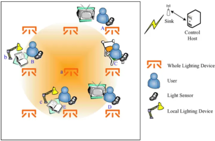
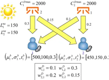
Fig. 1. The network scenario of our system.
proposed in [10] and [11] need to measure all combinations of dimmer settings and the resulting illuminations at all locations, so if there are interested locations, dimmer levels, and lighting devices, the measurement complexity is . In [9], for pervasive sensors deployment, the measuring time complexity was further reduced to . The goal was to satisfy users’ demands while optimizing energy efficiency. These works all relied on knowing users’ current locations, so extra localization mechanisms were needed.
In this work, we propose a light control system that considers both users’ preferences and energy conservation. Fig. 1 shows a typical network scenario in which users carry light sensors and lighting devices are controllable. Sensors can help each other to relay sensing data to the sink node. Then, the control host can give commands to lighting devices based on collected data. Here, we consider LED lighting devices [13], [14] and they are categorized into whole and local lighting devices. The former can provide background illuminations for multiple users in wide areas, and the latter is similar to desk lamps that provide con-centrated illuminations. For example, in Fig. 1, device in the center can provide background illuminations for user , and , and device can only provide concentrated illumination for user .
In our system, users may have different illumination require-ments according to their activities and profiles. Two types of requirements, background and concentrated ones, are consid-ered. For example, in Fig. 1, user is watching television, is reading a book, and is sleeping. Both and require the same background illuminations, but needs concentrated illumination. does not require neither background nor con-centrated illuminations. A user is said to be satisfied if the pro-vided background and concentrated illuminations fall into the required ranges. To evaluate the satisfaction level of a user, we 1530-437X/$26.00 © 2010 IEEE
further consider a binary satisfaction model and a continuous
satisfaction model. The former only returns a satisfaction value
of 1 or 0, while the latter returns a value between 0 and 1. We de-velop two algorithms to adjust whole lighting devices for these models with the goals of meeting users’ requirements while minimizing energy consumption. In case that it is impossible to satisfy all users simultaneously, we will gradually relax users’ requirements until all users are satisfied. For concentrated il-luminations, assuming that local lighting devices are moveable (which can be supported by robot arms), we develop a novel “surface-tracking” scheme to track local movements of users to provide required illuminations.
The main contributions of this work are twofold. First, our model is designed for “point-like” light sources, such as LEDs, which are more energy-efficient than traditional light sources and are expected to be the mainstream of lighting technologies in the future. We show how to take advantage of its light prop-agation property to conduct light control. Second, compared to existing solutions, our solution is “autonomous” in the sense that it can dynamically adapt to environment changes and does not need extra scheme to track users’ locations. Hence, our work re-laxes the requirement of an underlying localization mechanism in existing works.
The rest of this work is organized as follows. Section II presents the system model. Sections III and IV introduce our control algorithms for background and concentrated light sources, respectively. Section V contains simulation results. Section VI presents our prototyping results. Conclusions are drawn in Section VII.
II. SYSTEMMODEL
A. Light Measurement Method
In our system, there are users, , whole
lighting devices, , and local lighting
de-vices, . The lighting devices are controllable. For
all , user carries a light sensor which
pe-riodically reports an illumination level sensed by the sensor to the control host. The luminous intensity emitted by is de-noted by , and that by is denoted by . Considering physical limitations, we assume that and should satisfy
and .
We make the following assumptions in our work. First, there exists a natural light source, but it may change over time. Second, artificial light sources are assumed to be “point-like” ones such as LEDs. This makes modeling the impact of light sources easier. For whole lighting sources, disturbance from other objects may exist (such as furniture, obstacles, walls, etc.). However, we assume that it is possible to derive the impact of a whole lighting device on a sensor. That allows us to decide the proper intensity of each light source. For local lighting sources, we assume that no such disturbance exists. So, we can derive the distance between a lighting source and a user based on the measurement of light sensors. In addition, we assume that local lighting sources are mounted on robot arms and thus the position and orientation of local lighting sources are controllable. We will discuss more about this in Section IV. Next, we explain how to model the impact of a light source on a light sensor . Here, can be a whole lighting source
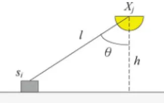
Fig. 2. Measuring the impact of a light sourceX on a light sensor s .
Fig. 3. An example of weight measurement.
or a local lighting source (See Fig. 2). Let and be the distances from to and to the nearest ground, respectively. Now let increase its intensity by candela, and we mea-sure the change of illumination at . According to the light propagation property, we have
(1) From and the observed , we define the impact of
on as
(2) Intuitively, this implies that even if and are unknown, we can still measure the weight from and . There-fore, we can easily decide the amount of increment/decrement on ’s intensity to achieve the desired level of illumination sensed by . Below, if , the impact is written as ; if , it is written as . The measurement of impact values should be done one-by-one, so the overall time com-plexity is . In comparison, this is much lower than those in [9], [10] and [11]. Besides, in our work, we can fur-ther consider measuring the impacts of some lighting devices and using interpolation techniques to estimate the impacts of remaining lighting devices to further reduce the measurement cost.
The key technique to the above weight measurement is to slightly increase each light source’s intensity one-by-one. In the example illustrated in Fig. 3(a), if increases 10 candela and the light intensities sensed by and increase by 1 and 2
lux, respectively, then we can get and
. Similarly, in Fig. 3(b), if increases 10 candela and the light intensities sensed by and increase
by 3 and 1.5 lux, then we can get and
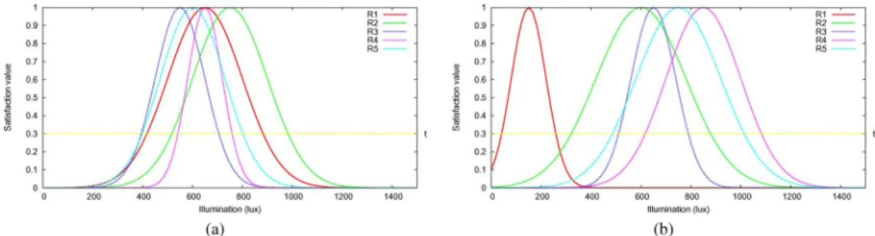
Fig. 4. An example of continuous satisfaction.
Because illuminations are additive [11], the light intensity sensed by , denoted as , is the sum of the natural light and the illuminations provided by the whole and local lighting devices, i.e.,
(3) is called the concentrated illumination perceived by , and the background illumination perceived by is estimated by . In this work, we consider two kinds of user satisfaction models for illuminations:
1) Binary satisfaction model: Each user has an accept-able background illumination interval and an acceptable concentrated illumination interval . The user is said to be satisfied if its concentrated and background illuminations fall within these intervals, respectively.
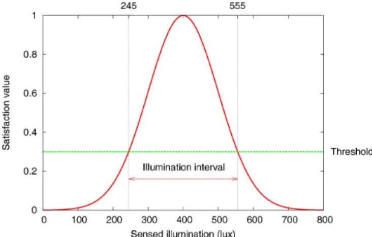
2) Continuous satisfaction model: Each user has concen-trated and background illumination requirements, but they are specified by utility-like functions.1 The satisfaction
value is given by a normal-distribution-like function with parameter , , and . If denotes the illumination, the satisfaction value is defined as given in (4) at the bottom of the page. For the background illumination (or the concentrated illumination, respectively), we denote the three parameters as , and (or , and , respectively). Fig. 4 shows an example of continuous
model with , , and .
Note that for concentrated illuminations, we assume that it is always possible to meet users’ requirements since local lighting devices are very close to users, so no particular model is specified.
1The work [11] adopts a curve function to represent users’ lighting
prefer-ences. In this work, we adopt Gaussian functions to represent users’ lighting preferences. However, it is not hard to extend to other utility functions.
B. Control Flow
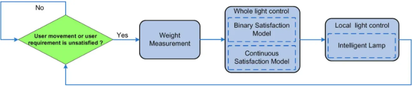
Fig. 5 illustrates the light control flow of our system. The con-trol process is triggered by user movement, periodical checking, or inputs from sensors which reveal that some users are not satisfied. Then, the weight measurement block determines and that had been discussed in Section II-A. After that, the whole light control and local light control modules follow. The background illumination constraints are achieved by tuning
for all users based on , and the
concen-trate illumination constraints are achieved by tuning for each
user based on .
It turns out that decisions of the whole or local light control can be made independently of each other.
III. CONTROL OFWHOLELIGHTINGDEVICES
In this section, we design two solutions for the binary and the continuous satisfaction models. For the binary satisfaction model, the primary goal is to meet all users’ requirements. Once the primary goal is met, the secondary goal is to minimize the total energy cost. It is possible that there exists no solution to meet all users’ requirements. In such a case, we can compro-mise by enlarging users’ acceptable intervals until all users are satisfied. The details of this issue will be discussed later. After the relaxation, we go to achieve the secondary goal, just like before. For the continuous satisfaction model, since users’ sat-isfaction values are represented by utility functions, there are not too many chances to further optimize the total energy cost. So, in this case, we only adjust light intensities to maximize the total satisfaction value of all users.
A. Binary Satisfaction Model
Our goal is to determine for device to meet users’ background illumination requirements. Under the binary satis-faction model, we are given the inputs including for all
and ; , and for all
; and for all . Our goal
is to solve for all with the objective function (5) subject to
(6) (7) Note that in (6), the can be known by the weight mea-surement method in Section II-A. In some cases, the initial value of is not zero. Hence, we can subtract the initial value to
if
Fig. 5. Light control flow chart.
get the adjustment value for each lighting device. Equation (5) is to minimize the total power consumption of whole lighting devices. Equation (6) imposes that all users’ background illu-mination requirements should be met. Equation (7) is to con-fine the adjustment result within the maximum and the min-imum bounds. Note that for all . This is a linear programming problem and can be solved by, e.g., the Simplex method [15]. Intuitively, the primary goal is to meet all users’ requirements. The secondary is to achieve (5). However, in re-ality, the system may be infeasible. One may try to eliminate the least number of requirements to find a feasible subsolution. However, it was shown that finding a feasible subsystem of a linear system by eliminating the fewest constraints is NP-hard [16]. So, we compromise by gradually relaxing users’ require-ments to make this problem feasible. Therefore, we propose an iterative process as follows. First, we run the Simplex method. If no feasible solution is found, we change ’s requirement to
for each , where
is a constant. Then, we run the Simplex method again. This is repeated until a solution is found. Once all users’ requirements are met, we go to minimize the total energy cost.
B. Continuous Satisfaction Model
Under the continuous satisfaction model, the inputs include
for all and ; and
for all ; and for all .
The goal is to find for all with the objective function
(8)
subject to
(9) (10) Equation (8) is to maximize the sum of satisfaction values of all users. Equation (9) imposes that all users’ background illu-mination requirements should be met. Equation (10) specifies the bounds. This is a nonlinear programming problem and can be solved by a sequential quadratic programming (SQP) method [17]. If there is no feasible solution, we gradually relax users’
Fig. 6. An example for the binary satisfaction model.
requirements to make this problem feasible. We propose an it-erative process as follows: First, we run the SQP method. If no feasible solution is found, we change ’s background threshold
to for each , where is a constant.
Then, we run the SQP method again. This is repeated until a so-lution is found.
C. Examples
An example of the binary satisfactory model is illustrated in Fig. 6, where there are two users and , and two whole
lighting devices and . We have , ,
, and . The
ob-jective function is
subject to
Since this problem is feasible, the solution is and . If the current light intensities are
and , we need to set
and .
Fig. 7 illustrates an example of the continuous satis-faction model. Similarly, there are two users and two
Fig. 7. An example for the continuous satisfaction model.
. We assume that
and for and ,
respec-tively. Given and , we can derive
and
for and , respectively. The objective function is
subject to
Again, this problem is also feasible. The solution is and . If the current light intensities are
and , we need to set
and .
IV. CONTROL OFLOCALLIGHTINGDEVICES
The above lighting control heuristic algorithms are able to adjust background illuminations to meet users’ needs. Here, we are further going to propose a robotic device, called
Intelli-gent Lamp (iLamp), to provide concentrated illuminations. An
iLamp has a robot arm with at least four local lighting devices and is supposed to serve one user who has need of concentrated illumination. The service scenario is shown in Fig. 8. The sensor should be placed on the reading surface. On detecting a user under its service area, the iLamp will compute its relative tion to the light sensor, move via its robot arm to a better loca-tion, and then adjust its luminous intensities to meet the need with the least energy. Detecting a nearby user is a simple job since a local lighting device can check if it has non-negative impact on a sensor.
Given an iLamp and a light sensor , they will cooperate with each other by the following four steps to achieve our goal: 1) col-lect the current sensed by ; 2) calculate the location of ;
Fig. 8. Service scenario of an iLamp and a light sensor.
Fig. 9. The geometry model of iLamp to track the location ofs .
3) adjust the lamp’s robot arm; and (4) adjust the luminous in-tensities of its lighting devices. Step 1 is executed periodically. Once it finds that the current illumination falls outside the re-quired interval, steps 2, 3, and 4 are triggered. Central to our scheme is step 2, so we will elaborate it in more details below.
To drive step 2, assume for simplicity that the iLamp has four local lighting devices , , , and as shown in the ge-ometry model in Fig. 9(a). Note that it is not hard to extend this result to more lighting devices in other geometry models. Since there is a robot arm, the iLamp should know the
coordi-nate of , . Without loss of generality,
, the projection of on the surface as the axis, the projection of on the surface parallel with the axis, and the norm of the surface toward the sky as the axis. Let the location of be . We will derive a scheme to find its location as follows. Since LED is a point-like light source, it dissipates identically in all directions. Our scheme consists of two symmetric processes. The first one is to use and to estimate two potential locations of , and then use and to screen out one location. The second one is to use and to estimate two potential locations of , and use and to screen out one location. Finally, we take their middle point as the estimated location of .
1) For each , , increase its luminous intensity by candela and measure the change of illuminance intensity at , denote by . According to the definition of illumination, we have the equality
where
This leads to
(11)
2) Observe that the equations of and represent two balls centered at and , respectively. Since it is known that , each of these two balls intersects with plane at a circle. These two circles will intersect at two points. Using any equation of and , we can pick one point as the estimated location of , called . [Refer to Fig. 9(b).]
3) Similarly, the equations of and represent two balls at and , respectively, each intersecting with plane at a circle. Again, these two circles intersect at two points, and we can pick one point as the location of , called , with the assistance of and .
4) Finally, the location of is predicted as the middle point
of and .
In step 3, we move our lighting devices toward the upper side of . This includes two substeps. First, we rotate the robot arm by angle such that the vector from to , after projecting to the reading surface, is pointing toward the location of . Second, it moves to the upper side of to provide a proper reading angle (a typical angle is 60 ).
Step 4 is to adjust , to meet the concentrated illumination demand of . From the results in Section III, some background and natural illuminations have already been pro-vided. So we only need to add some more light to meet ’s need. The results in Section III can be directly applied again here, so we omit the details.
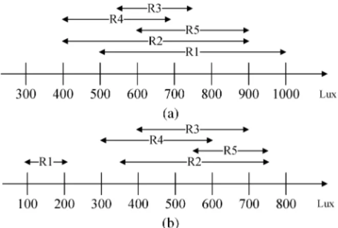
Fig. 10. Requirement pools: (a)RP 1 and (b) RP 2.
V. SIMULATIONRESULTS
To understand how our schemes for whole lighting control meet users’ requirements while saving energy, we have devel-oped a simulation. Two scenarios are considered. One scenario, denoted as , is in a room of size 10 10 with an array of 5 5 whole lighting devices. The other scenario, denoted as , is in a room of size 20 20 with an array of 9 9 while
lighting devices. We set and for all
. Our proposed algorithms are compared to other two schemes, called FIX and GREEDY. The FIX scheme is a very intuitive one assuming that users’ locations are known in advance. The nearest devices are selected and set to a fixed candela value . We denote this scheme as FIX- below. The GREEDY scheme also assumes that users’ locations are known. For each user, the nearest device is selected to satisfy the user (if possible). If it is still below the required illumination, the second nearest device is picked to increase the intensity. This is repeated until the user is satisfied. Note that it may happen that a user is satisfied first but later on becomes unsatisfied due to other devices change their intensities. Below, we compare the outcomes according the two satisfaction models introduced in Section II.
• Binary satisfaction model: A requirement pool is a set of requirements. In the simulation, each user will randomly choose one from the pool as its requirement. Two require-ment pools, denoted by and , are considered. See Fig. 10 in which each range represents an expected il-lumination interval. We consider two performance indices here. The first index is the total energy consumption. The second index is called GAP, which reflects the difference between the provided illumination and the required one. The GAP for user is
if
otherwise. (12) We will measure the average GAP of all users.
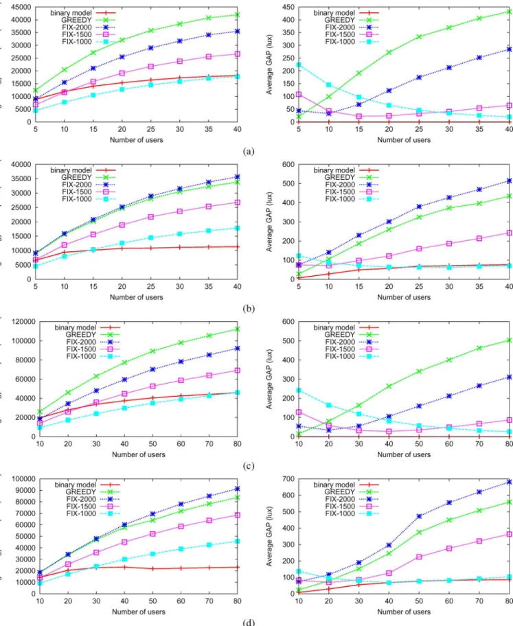
Fig. 11 shows our simulation results under different
com-binations of and . In Fig. 11(a), we see
that our scheme is the most energy-efficient while keeping the average GAP close to zero. This is because the re-quirement intervals in have common overlapping and that allows our system to satisfy all users in most cases. Note that although FIX-1000 uses less energy, its GAP is
Fig. 11. Comparison under the binary satisfaction model: (a) network scenarioS1 and pool RP 1, (b) network scenario S1 and pool RP 2, (c) network scenario S2 and pool RP 1, and (d) network scenario S2 and pool RP 2.
much larger. Fig. 11(b) adopts . Because some re-quirements are violated, our scheme also induces some GAP. However, our scheme is also the most
energy-effi-cient. Fig. 11(c) and (d) are the case of and the trends are similar. This demonstrates that our scheme is quite scal-able to network size.
Fig. 12. Requirement pools: (a)RP 3 and (b) RP 4.
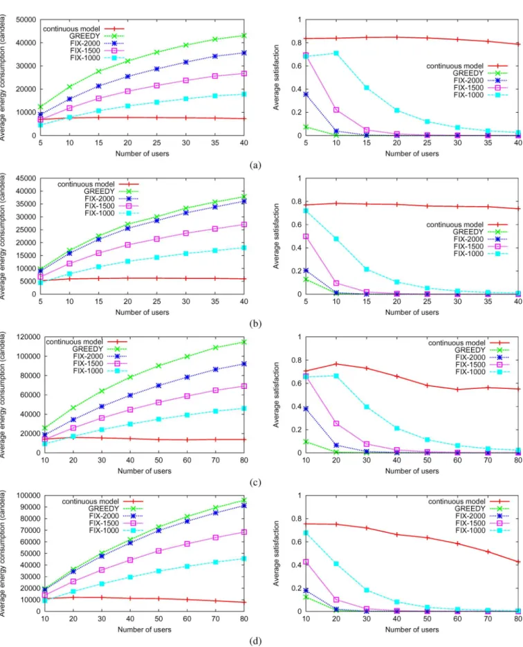
• Continuous satisfaction model: We define two require-ment pools and , as shown in Fig. 12. Note that has higher deviation in requirements than . The satisfaction threshold is set to 0.3. We compare two performance indices: average user satisfaction and energy consumption. Fig. 13 shows our simulation results under
different combinations of and . These
results consistently indicate that our scheme provides the highest satisfaction levels and outperforms FIX and GREEDY schemes in energy consumption.
VI. PROTOTYPINGRESULTS
We have developed a prototype to verify our designs. Fig. 14 shows the system architecture. Users carry a badge with a built-in light sensor. The user’s preference can be configured via the badge. The control host can make decisions and send them to lighting devices. We test our system in a room of size 8 6 with whole lighting devices deployed in a grid manner. Some demo videos of our work can be found at http://hscc.cs.nctu.edu.tw/iLight/. Below, we introduce each device, and then give our testing results.
A. User Badge and Light Sensor
The user badge has a wireless module Jennic (JN5139) [18], a light sensor (TSL230) [19], a TFT LCD panel (ILI9221) [20], and some input buttons. JN5139 is a single-chip microprocessor with an IEEE 802.15.4 [21] module. Fig. 15(a) illustrates the front and back views of the user badge. The outlook of a badge is like a bookmark. Users can specify their preferences via our graphic user interface (GUI) and buttons.
B. Whole Lighting Device
We use LEDs as light sources and deploy them on the ceiling. As shown in Fig. 15(b), each whole lighting device has a 4 4 LED module and a thermal pad is attached on its back for heat dissipation. We adopt pulse width modulation of digital input/ output (DIO) to control the luminous intensity of light sources. Each LED has 20 levels of illumination, ranging from 0% to 100% luminous intensity. Fig. 15(c) shows our prototype.
C. iLamp
Fig. 15(d) shows the iLamp, which is composed of a robot arm, four sets of LEDs, and a JN5139 module. The robot arm consists of six Dynamical AX-12 actuators [22] as the lamp
holder. Each AX-12 actuator can rotate from 0 to 300 at an ac-curacy of 0.33 . LEDs are similar to those used in whole lighting devices and with 20 levels of illuminations.
D. Control Host
Implemented by JAVA, the control host is the core of our system. It is composed of three components, including the User
Status Tracker, Decision Handler, and Device Controller. By
applying Java thread programming techniques, tasks are han-dled concurrently.
• User Status Tracker: This component checks current illu-minations of all users periodically and, when needed, up-dates users’ requirements. If it finds that a user’s require-ment is not satisfied or is updated, the Decision Handler will be triggered.
• Decision Handler: This component realizes our control algorithms. It is triggered by the User Status Tracker. The linear and nonlinear programming are resolved by the MATLAB Builder for Java [23]. The results are sent to the Device Controller to adjust lighting devices
• Device Controller: This is the interface between the control host and actuators. Commands are sent via RS232.
E. Performance Verification
We first verify the correctness of (1) through some tests. In Fig. 16(a), we fix and and vary from 30 to 230 cm. We measure the received illumination (in dash lines) and derive the ideal illumination (in solid line). The distance error between ideal and real values are calculated (in bars). As can be seen, the distance error is bounded by 10 cm. In Fig. 16(b), we fix and and vary from 40 to 400. We measure and calculate the distance error. Again, the gaps between the real distance and the derived distance are quite small.
Next, we verify our results in a real environment. We place 20 whole lighting devices in a 8 6 room in a grid-like manner. We adopt the same performance indices introduced in Section V. In Fig. 17, we compare the simulation and implemen-tation results where there are 1 to 5 users. Each user may ran-domly select a requirement from requirement pools and for the binary satisfaction model or and for continuous satisfaction model. In all performance indices (av-erage energy consumption, GAP, and satisfaction), the differ-ence between simulation and implementation results are very close. The results indicate the correctness of our approaches. We further validate our results under different weather conditions, which may reflect to different nature light scenarios. Fig. 18
Fig. 13. Comparison under the continuous satisfaction model: (a) network scenarioS1 and pool RP 3; (b) network scenario S1 and pool RP 4; (c) network scenarioS2 and pool RP 3; and (d) network scenario S2 and pool RP 4.
shows the results by using the measured natural light as the index. We fix the number of users to three and randomly select their lighting requirements. There still exists high consistency
between simulation and implementation results in most cases. Also, when the average natural light increases, the gap in en-ergy consumption tends to become smaller.
Fig. 14. Hardware and software system architecture of our prototype.
Fig. 15. (a) Front and back views of user badge, which looks like a bookmark; (b) whole lighting device; (c) testing environment; and (d) iLamp.
Fig. 16. Verification of (1): (a) fixingh and 1C and varying l and (b) fixing h and l and varying 1C .
For iLamp, we place a book on the desk and attach the light sensor on the book. We try to move the book (i.e, move the light sensor) from time to time. In this experiments, the is set to 12.25 candela. The average time for executing the algorithm of
iLamp are about 3 seconds. (Steps 1 and 2 take about 1 second, and steps 3 and 4 take about 2 seconds.) This experiment shows that the amount of error of the angle pointing toward the light sensor is less than 15 .
Fig. 17. Comparison of simulation and real implementation results under different numbers of users: (a) binary satisfaction model and poolRP 1 or RP 2, and (b) continuous satisfaction model and poolRP 3 or RP 4.
Fig. 18. Comparison of simulation and real implementation results under different natural light: (a) binary satisfaction model and poolRP 1 or RP 2 and (b) continuous satisfaction model and poolRP 3 or RP 4.
VII. CONCLUSION
We have presented an autonomous light control system. Both whole and local lighting devices are considered. For controlling whole lighting devices, two decision algorithms are proposed. For controlling local lighting devices, a novel surface-tracking scheme is proposed. Our system can dynamically adapt to envi-ronment changes and improve our earlier works by eliminating the requirement of tracking users’ current locations. We eval-uate our algorithms by simulations under different configura-tions. Besides, we have developed prototypes and deployed the whole system in a room to verify its effectiveness under real conditions. The results do show high consistency.
There is a basic limitation in our system. We enforce that users must carry light sensors to measure their current light in-tensities. This is due to the nature of light propagation. Without these light sensors, our system cannot get any information nearby the users. There are some alternatives, such as using motion sensors or thermal sensors to detect users’ locations or rough light environments, respectively. Unfortunately, such approaches still cannot provide satisfactory solutions so far.
In Section III-B, we adopt Gaussian functions to represent users’ satisfaction levels. However, the utility to human, in terms of light intensity, is still an unknown factor. This may deserve further study in the medical science field.
REFERENCES
[1] H.-W. Gellersen, A. Schmidt, and M. Beigl, “Multi-sensor context-awareness in mobile devices and smart artifacts,” ACM/Kluwer Mobile
Networks and Applications, vol. 7, no. 5, pp. 341–351, 2002.
[2] M. Haenggi, “Mobile sensor-actuator networks: Opportunities and challenges,” in Proc. IEEE Int. Workshop on Cellular Neural Networks
and their Applications, 2002, pp. 283–290.
[3] Y.-C. Tseng, Y.-C. Wang, K.-Y. Cheng, and Y.-Y. Hsieh, “iMouse: An integrated mobile surveillance and wireless sensor system,” IEEE
Computer, vol. 40, no. 6, pp. 60–66, 2007.
[4] X. Wang, J. S. Dong, C. Chin, S. Hettiarachchi, and D. Zhang, “Se-mantic space: An infrastructure for smart spaces,” IEEE Pervasive
Computing, vol. 3, no. 3, pp. 32–39, 2004.
[5] S.-P. Kuo and Y.-C. Tseng, “A scrambling method for fingerprint positioning based on temporal diversity and spatial dependency,”
IEEE Trans. Knowledge Data Eng., vol. 20, no. 5, pp. 678–684,
2008.
[6] D. Niculescu and B. Nath, “Ad hoc positioning system (APS) using AOA,” in Proc. IEEE INFOCOM, 2003, pp. 1734–1743.
[7] A. Mainwaring, D. Culler, J. Polastre, R. Szewczyk, and J. Anderson, “Wireless sensor networks for habitat monitoring,” in Proc. ACM Int.
Workshop on Wireless Sensor Networks and Appl. (WSNA), 2002, pp.
88–97.
[8] G. Werner-Allen, J. Johnson, M. Ruiz, J. Lees, and M. Welsh, “Moni-toring volcanic eruptions with a wireless sensor network,” in Proc. Eur.
Workshop on Sensor Networks (EWSN), 2005, pp. 108–120.
[9] M.-S. Pan, L.-W. Yeh, Y.-A. Chen, Y.-H. Lin, and Y.-C. Tseng, “A WSN-based intelligent light control system considering user activities and profiles,” IEEE Sensors J., vol. 8, pp. 1710–1721, 2008. [10] H. Park, M. B. Srivastava, and J. Burke, “Design and implementation
of a wireless sensor network for intelligent light control,” in Proc. Int.
Symp. Inf. Process. Sensor Networks (IPSN), 2007, pp. 370–379.
[11] V. Singhvi, A. Krause, C. Guestrin, J. H. Garrett, and H. S. Matthews, “Intelligent light control using sensor networks,” in Proc.
ACM Int. Conf. Embedded Networked Sensor Syst. (SenSys), 2005,
pp. 218–229.
[12] Y.-J. Wen, J. Granderson, and A. M. Agogino, “Towards embedded wireless-networked intelligent daylighting systems for commercial buildings,” in Proc. IEEE Int. Conf. Sensor Networks, Ubiquitous, and
Trustworthy Computing, 2006.
[13] LED Lamp. [Online]. Available: http://en.wikipedia.org/wiki/ LED_lamp
[14] Light-Emitting Diode (LED). [Online]. Available: http://en.wikipedia. org/wiki/LED
[15] T. H. Cormen, C. E. Leiserson, and R. L. Rivest, Introduction to
Algo-rithms. Cambridge, MA: MIT Press, 2001.
[16] J. Sankaran, “A note on resolving infeasibility in linear programs by constraint relaxation,” Oper. Res. Lett., vol. 13, no. 1, pp. 19–20, 1993.
[17] P. T. Boggs and J. W. Tolle, “Sequential quadratic programming,” Acta
Numerica, vol. 45, no. 1, pp. 1–51, 1995.
[18] Jennic, JN5139. [Online]. Available: http://www.jennic.com/ [19] Light Sensor, TSL230. [Online]. Available: http://www.taosinc.com/ [20] TFT LCD, ILI9221. [Online]. Available:
http://www.ilitek.com/prod-ucts.asp
[21] IEEE Standard for Information Technology – Telecommunica-tions and Information Exchange Between Systems – Local and Metropolitan Area Networks Specific Requirements Part 15.4: Wireless Medium Access Control (MAC) and Physical Layer (PHY) Specifications for Low-Rate Wireless Personal Area Networks (LR-WPANs) 2003.
[22] AX-12, Dynamixel Series Robot Actuator. [Online]. Available: http:// www.crustcrawler.com/motors/AX12/index.php
[23] Matlab Builder for Java. [Online]. Available: http://www.mathworks. com/products/javabuilder/
Lun-Wu Yeh received the B.S. and M.S. degrees in
computer and information science from the National Chiao-Tung University, Hsin-Chu City, Taiwan, in 2003 and 2005, respectively. He is currently working towards the Ph.D. degree at the Department of Computer Science, National Chiao-Tung University. His research interests include smart living space and wireless sensor network.
Che-Yen Lu received the B.S. and M.S. degrees
in computer and information science and computer science from the National Chiao-Tung Univer-sity, Hsin-Chu City, Taiwan, in 2007 and 2009, respectively.
His research interests include wireless sensor net-work and wireless communication.
Chi-Wai Kou received the B.S. degree from the
National Tsing-Hua University, Hsinchu, Taiwan, in 2008. He is currently working towards the M.S. degree at the Department of Computer Science, National Chiao-Tung University, Hsin-Chu City, Taiwan.
His research interests include wireless communi-cation and sensor networks.
Yu-Chee Tseng (SM’03) received the B.S. and
M.S. degrees in computer science from the National Taiwan University and the National Tsing-Hua University, Hsinchu, Taiwan, in 1985 and 1987, respectively, and the Ph.D. degree in computer and information science from the Ohio State University Columbus, in January 1994.
He was an Associate Professor at the Chung-Hua University (1994–1996) and at the National Central University (1996–1999), and a Professor at the Na-tional Central University (1999–2000). Currently, he is Chairman of the Department of Computer Science, and Associate Dean of the College of Computer Science, National Chiao-Tung University, Taiwan.
Dr. Tseng is a member of ACM. He received the Outstanding Research Award by the National Science Council, R.O.C., in both 2001–2002 and 2003–2005, the Best Paper Award by the International Conference on Parallel Processing in 2003, the Elite I. T. Award in 2004, and the Distinguished Alumnus Award by the Ohio State University in 2005. His research interests include mobile com-puting, wireless communication, network security, and parallel and distributed computing.
Chih-Wei Yi (M’04) received the B.S. and M.S.
de-grees from the National Taiwan University, Taipei, in 1991 and 1993, respectively, and the Ph.D. degree from the Illinois Institute of Technology, Chicago, in 2005.
He is currently an Associate Professor of Com-puter Science at the National Chiao-Tung University. He was a Senior Research Fellow of the Department of Computer Science, City University of Hong Kong. His research focuses on wireless ad hoc and sensor networks, vehicular ad hoc networks, network coding, and algorithm design and analysis.
Prof. Yi is a member of ACM. He received the Outstanding Young Engineer Award from the Chinese Institute of Engineers in 2009.