高光譜資料中都市地表物質的辨別 

高光譜資料中都市地表物質的辨別

Discrimination of Urban Surface Materials in Hyperspectral Data

陳哲銘

Che-Ming Chen2 George F. Hepner3

Abstract

Conventional multispectral data associated with statistical data-driven methods are ineffective for extracting urban land cover information in detail due to the insufficiency on spectral and spatial resolution. In this research, an urban spectral library is established to provide the field spectra and the related spectroscopic knowledge of urban surface materials. A pixel-based spectral analysis algorithm, spectral angle mapper (SAM), is adopted to identify urban surface materials in low-altitude AVIRIS data (224 bands, 2.9 m spatial resolution) by matching image spectra to field spectra. The results confirm the imaging spectroscopic approach using low-altitude hyperspectral data associated with pixel-based spectral analysis can identify many urban surface materials, which are indistinguishable in the conventional multispectral data. The surface material map derived from this approach is better suited to meet the information requirements of a broader set of urban applications.

Keywords: urban spectral library, urban surface material, spectral angle mapper, AVIRIS, imaging spectroscopy

*1 _{本研究初步成果曾於 2001 年美國太空總署噴射推進實驗室(NASA Jet Propulsion Laboratory)}

AVIRIS Earth Science and Applications Workshop 口頭發表

2 _{國立台灣師範大學地理系副教授(通訊作者)}

中文摘要

受限於光譜和空間解析力，藉由統計方法在傳統多光譜影像中擷取資料的方 式，難以獲取詳細的都市土地覆蓋資訊。本研究透過建立一個都市光譜資料庫來 搜集都市地表物質的地面光譜與其相關的光譜知識，並以「光譜角度分類法」 （spectral angle mapper, SAM）匹配低空 AVIRIS 影像（具有 224 個波段，空間解 析力 2.9 公尺）中的像元光譜與光譜資料庫中的地面光譜來進行地物辨認。研究結 果證實，藉由低空的高光譜資料搭配像元式的光譜分析，應用成像光譜分析法能 辨別出許多在傳統多光譜資料中無法分辨的都市地表物質，因此能符合在都市應 用上更廣泛的資訊需求。 關鍵詞：都市光譜資料庫、都市地表物質、光譜角度分類法、AVIRIS、成像光譜 分析法

Introduction

Recently, several global change reports describe the need for regional scale assessments of human vulnerability and ecosystem sustainability to activities concentrated in and near urban areas (IGBP, 1995). The investigations of global environmental change have given great attention to the role of urban areas as regional growth poles of environmental degradation (Hepner et al., 1998). There is widespread interest in the development of urban information systems for the collation, assessment, and practical utilization of urban data from a variety of sources. Urban geographers and planners recognize remote sensing data as a vital part of the total information pool (Barrett and Curtis, 1992). Remote sensing analysis provides a basis for studies in urban morphology, biophysical systems, and human systems, which serve the purposes of science, environmental management, and urban planning (Ridd, 1995).

Although urban analysis is one of the most common applications of remote sensing, the information derived from remotely sensed data is often insufficient for operational use. One of the main problems is that the spectral and spatial resolution of sensors are too coarse to extract the desired information for urban analysis (Hepner et al., 1998). For example, neither Landsat TM nor SPOT has been shown to distinguish urban soils and impervious surfaces adequately (Ridd et al., 1992). In addition, the spatial resolution (10 to 30 m) of Landsat TM and SPOT data is a limitation for extracting urban land cover information. High spatial resolution sensors, such as Ikonos, provide high spatial resolution, but have limited spectral information. Generally, sensors with a spatial resolution of approximately 5 to 20 m are required to obtain USGS Level II information (Jensen and Cowen 1999). The low spatial resolution results in the spectral mixture problem and complicates the classification. Therefore, both high spectral and spatial resolution are required to differentiate complexity of the urban land covers and surface materials.

The spectral resolution of remotely sensed data is, in practice, related to its spatial resolution. With low spatial resolution, many urban surface materials are located in the field of view of sensors. The combined signal is dominated by the brighter component (Clark, 1999). However, the spectral reflectance shape, the intensity of reflectance, and the width and depth of absorption features of the brighter component may have changed. These mixed pixels would be misinterpreted or unclassified. Theoretically, there are two ways of resolving the spectral mixture problem. The first, the most efficient way, is to improve the spatial resolution because the pixel purity is increased while the amount of materials is decreased in the field of view. The second approach is to apply subpixel analysis that can model or detect the abundance of components in a pixel.

and the Airborne Visible InfraRed Imaging Spectrometer (AVIRIS), have been developed since the 1980s. An imaging spectrometer with 10 nm contiguous bands and 400- to 2500-nanometer spectral range can produce data with sufficient spectral resolution for the direct identification of most earth surface materials with diagnostic absorption features. The hyperspectral data created by these spectrometers have been used initially in geological, aquatic and later ecological and atmospheric investigations (Curran, 1994). However, hyperspectral data have been used sparsely for the study of urban areas (Ridd et al., 1992; Hepner et al., 1998). There is a potential to resolve the spectral ambiguity of urban surface materials which are not differentiable in the broadband data using the imaging spectroscopic approach.

Information extraction from hyperspectral data such as AVIRIS, spectral analysis, typically employs reference spectra from a spectral library or the endmembers derived from the images to match against the image spectra. These can be used to exploit the continuity of spectral information available with imaging spectrometers. There are many algorithms developed for spectral analysis. The specific approach selected must correspond to the objectives of analysis and the spectral characteristics of the surface material targets. The optimal techniques for extracting urban surface materials from the hyperspectral data should be identified by examination of the spectral and contextual characteristics of surface materials in the urban scene.

Previous urban studies using remote sensing have been plagued by ambiguity in feature and surface material definiton due to the limited spectral and spatial resolution. This research attempts to investigate this fundamental problem using a higher spatial resolution imaging spectroscopic approach. The research objectives include:

 Investigate the potential utility of imaging spectroscopy in urban surface material characterization. The low-altitude AVIRIS data, which provide

both high-spectral and high-spatial resolution, are employed to evaluate the feasibility of the imaging spectroscopic approach for directly extracting the surface materials in urban areas.

 Examine the spectral variability of urban field spectra from different ground collection sites. Signature extension has been commonly used by remote sensing researches to classify unknown pixels in a given scene by comparing their spectral properties to a spectral library containing spectral signatures of each class. The assumption of this approach is that the spectral signatures are identical from place to place for a given surface material. The components of spectral variability of field spectra in the study area are investigated to examine this assumption and assess the feasibility of the signature extension approach for hyperspectral data.

 Explore the appropriate analytical strategy for identifying urban surface materials. By analyzing spectral signatures of urban surface materials, the analytical strategy feasible for differentiating the urban surface materials in hyperspectral data can be determined.

Study Area and Data Acquisition

Study area

The urban area of Park City, Utah is used as the study area due to the representative mixture of land covers / surface materials for western U.S. cities. Although Park City area is not large, it contains a diversity of land covers, surface materials, and vegetation associations. Several land cover categories are common to nearly every urban area. These categories are light inert material (e.g., bare soil, concrete, reflective metals), dark inert material (e.g., membrane roofs, slag piles),

asphalt, water, annual weeds and natural grass areas, moist healthy vegetation, trees and shrubs, and mixed cover types. Most of these land covers can be found in the Park City area. It also provides the typical example where urbanization spreads from lowlands to adjacent uplands. Therefore, the methodologies, spectral signatures and techniques, which are investigated in this project, should then be transferable to other cities in the western U.S. and other semi-arid urban areas around the world.

Hyperspectral Data Acquisition

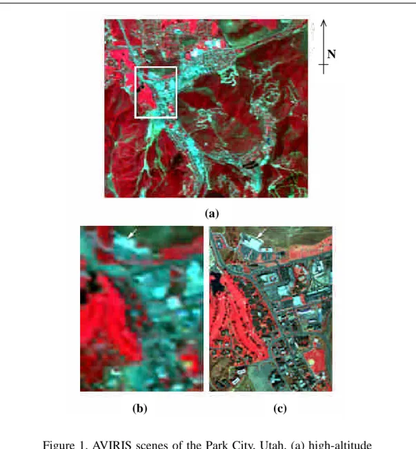
The high-altitude （20m spatial resolution）AVIRIS data of Park City area was obtained from the Park City flight on 5 August 1998. The data range for this imagery is from Band 1, with a bandcenter of 369.07 nm, to Band 224, with a bandcenter of 2507.50 nm. The low-altitude （2.9m spatial resolution）AVIRIS data were obtained on 19 October 1999. The common area of these two datasets is located at Prospector Square area in the Park City (Figure 1).

Since there is no feasible ground calibration site under this low-altitude AVIRIS flight, the high-altitude AVIRIS data are first corrected and then used to simulate the ground truth for calibrating the low-altitude AVIRIS data. A radiative transfer model (ATREM) was applied to the radiance data to remove the solar spectral response, atmospheric absorptions, and atmospheric scattering. The path radiance scattering was overcorrected by the ATREM resulting in the surface reflectance below 0 in the UV wavelengths. This was corrected by the use of an offset parameter provided by the USGS. Other artifacts of the spectra, which are small-scale spikes irresolvable by the ATREM, were also corrected by the multiplier parameter provided by the USGS derived from their nearby ground calibration site.

scene was selected and then edited to remove the residual atmospheric absorptions (Figure 1a, 1b). The ATREM calibration and path radiance correction were applied to the low-altitude AVIRIS data. Then the same pixels, which cover approximately 6 by 6 pixels in the low-altitude scene over the supermarket roof, were sampled and averaged to provide the spectrum. This low-altitude spectrum was divided into the edited high-altitude spectrum to obtain the multiplier used to calibrate the low-altitude data. This method had been validated by the USGS-EPA Imaging Spectroscopy Project (Rockwell et al., 1999; Rockwell, 2000).

Field Data Collection

A spectral library containing the reference spectra and the related spectroscopic knowledge of the urban surface materials was required to perform the spectral analysis. Although existing spectral libraries provide many urban surface materials, their diversity is not enough for this study. Use of the reference spectra to separate plant species, as well as humanmade materials, varies from one region to another and might decrease as the geographic area covered increases. Thus, a local spectral library of Park City was built to better match the AVIRIS data for the spectral analysis (Table. 1). This study used the JPL Spectral Library and other libraries of laboratory samples in conjunction with field and image spectra.

During the summer and autumn of 2000, 80 urban surface materials including 20 roofing materials, 12 paving materials, 23 vegetation, and other 25 materials, were measured in 9 field collection sites around the study area using an ASD field spectrometer with a 20-degree foreoptic. This spectrometer measures the targets with ground field of view (GFOV) about 0.5 m in diameter from a distance of shoulder height. At least 10 sample spectra for each target material were collected and averaged

to obtain representative spectral signatures. Some field spectra (e.g., riparian vegetation and flat rooftops), which could not be measured from ground due to lack of access or a prohibitive viewing angle, were measured from a helicopter flight on 27 September 2000 using the same field spectrometer with a 1-degree foreoptic. The flight height was maintained at 300 feet over the urban area and 400 feet over the suburban area. The GFOVs are 1.6 m and 2.1 m in diameter from the distance of 300 feet and 400 feet, respectively. The reflectance of these field spectra was rescaled to the magnitude of 0 to 1. Since the unit of wavelength, bandwidth, and bandcenter of field spectra are different from those of the AVIRIS data, the field spectra were resampled to correspond to the wavelength and FWHM of low-altitude AVIRIS data. The locations of field spectra were recorded using a GPS unit, and the digital photographs of each material were also taken using a digital camera. In the spectral library, the collection time of each target was used as a common index to integrate the multiple data sources. The field spectra were also registered onto the geocoded AVIRIS image.

Field Data Analysis

The selection of spectral analytical strategy to discriminate the urban surface materials is tied to spectral reflectance characteristics of the target materials. For example, if the targets have apparent absorption features, an absorption feature mapping algorithm would be appropriate (Mustard and Sunshine, 1999). Therefore, the spectral signatures of the most common surface materials in an urban environment were systematically examined before determining the analytical strategy.

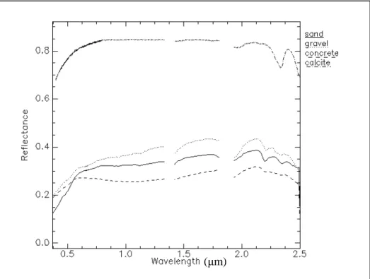
In the spectrum of concrete, there are two weak absorptions, 2.2 and 2.35µm, in the mid-infrared region. The absorption features in this region were caused by vibration processes occurring in some of the molecular groups that constitute minerals and rocks. The spectra of the main components of concrete, white sand, gravels, and carbonates, are examined (Figure 2).

Lime is the major ingredient of cement and is made by limestone and other forms of calcium carbonate (Microsoft, 2001). Since pure limestone consists of almost entirely of calcite, the absorption feature of calcite is found in the spectrum of cement. The absorption near 2.35 µm in the calcite (CaCO3) is due to the overtone (3v3) of the CO3 fundamentals (Clark, 1999). This feature can also be found in the spectra of sand and gravel involving vibrations of the carbonate group (Hunt, 1979). However, the absorption features in the spectra of sand and gravel are much weaker than that of calcite spectrum. The spectrum of calcite obtained from the JPL spectral library of laboratory samples is much purer than the field spectra. Therefore, the absorption feature of the lab spectrum is much stronger than the field spectra. In addition, the mineral sample in the JPL spectral library was ground to <45 µm grain size. Therefore, the amount of light scattered and absorbed by these small grains is much greater than those of the field samples (sand, gravel, and concrete). There is another absorption feature near 2.2 µm in the field spectra of sand and gravel. This feature is considered to be due to the combination of the OH stretch with the fundamental AlOH bending mode (Hunt, 1977).

In general, the absorption feature near 2.35 µm in the concrete spectrum can be explained by the carbonate group (2.35 µm) contributed by lime, sand, and gravel. The 2.2 µm absorption can be attributed to sand and gravels containing constituent OH groups. When these materials are mixed together, the spectra of sand and gravel

suppressed that of calcite in the spectrum of concrete. Furthermore, the absorption depths and widths of their individual composition is flattened and broadened in the concrete spectrum. The reflectance of the concrete is lower than each of its individual compositions through the visible to mid-infrared range. In comparing three concrete samples collected from different sites, their spectral curves are almost identical. Two very weak absorptions found at 0.95 and 1.15 µm on one of the samples are artifacts caused by the instrument noise of the field spectrometer (Figure 3).

Asphalt

Almost all of the asphalt used commercially is now derived from petroleum. Straight-run asphalts, which are made up of the nonvolatile hydrocarbons left after petroleum has been refined into gasoline and other products, are used for paving. The asphalt cement is heated, combined and mixed with the aggregate such as stone, sand, or gravel at a Hot Mix Asphalt facility (Microsoft, 2001).

When an intimate mixture occurs, the darker material will dominate the signal because photons are absorbed when they encounter a darker grain. It can be expected that the spectrum of asphalt would be dominated by the spectrum of nonvolatile hydrocarbons.

There are four distinct absorption bands at 1180 nm, 1380 nm, 1680 nm and 2300 nm in the near- and mid-infrared range in the spectrum of hydrocarbons (Clark, 1999). Among these four absorptions, the 2300nm has the strongest absorption reaching 95 percent absorption in the spectrum of crude oil (McCoy, unpublished data, 2000). This result confirms the above assumption that the common weak absorption near 2.3 µm among the spectra of asphalt was contributed by hydrocarbons. However, the absorption depth of the asphalt spectrum at 2.3 µm is much weaker than that of the

spectrum of crude oil. Since asphalt is the mixed material consisting of 5% hydrocarbons and 95% aggregates, the absorption depth, related to the abundance of hydrocarbon absorbers, significantly decreased.

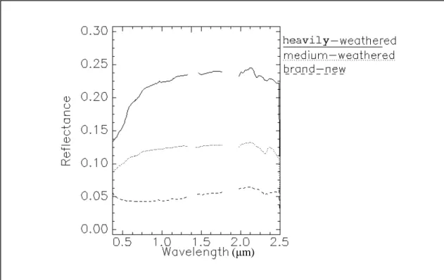
The field spectra of asphalt collected at the different sites have spectral variability. Paving asphalt in different ages or conditions may slightly change the spectral reflectance and, thus, can be detected by the field spectrometer (Figure 4). In comparing the paving asphalt samples measured at the different sites, the heavily-weathered sample revealed its gravel aggregates to the surface and little soil also covered it. A weak absorption feature near 2.2 µm is due to soil or gravel covering, which does not appear in the medium-weathered and brand-new asphalt samples. The reflectance of the new sample was 20% lower than the heavily-weathered sample. In addition, the spectral curve of the new asphalt sample is concave, which is different from the convex of heavily-weathered sample. The medium-weathered asphalt has a spectral curve in between the heavily-weathered and the new samples.

Vegetation

Since the high-altitude AVIRIS data were obtained in August, and the low-altitude AVIRIS data were obtained in October, the plant spectra were field measured both in summer and autumn to correspond to the image spectra. Species can be differentiated from each other by the leaf spectra collected in the summer (Figure 5). The chlorophyll absorptions in the visible region (0.45 to 0.52µm and 0.63 to 0.69µm), the magnitude of red edge (near 0.7µm), the broad absorptions near 1.73µm, 2.1µm, 2.3µm due to leaf biochemicals and the magnitude of the leaf water content from 2.1µm to 2.3 µm apparently differentiate dry grass and sagebrush from the other plants. Sagebrush has stronger chlorophyll absorption than dry grass near 0.66 µm. Healthy grass has the

highest reflectance at 0.9 and 1.1 µm. Blue spruce has the lowest reflectance from 2.1 to 2.3 µm. Regarding the leaf spectra of the same plants collected in the autumn, the stronger red reflectance and the weaker near infrared reflectance made alfalfa and aspen easier to discriminate in fall than in summer (Figure 6).

Water

In broadband data, water and asphalt usually are confused due to low reflectance. However, the field spectra show that water has apparent fluctuation in the visible region due to suspended and underwater materials. In comparing the field spectra of four water samples collected from a swimming pool, two ponds, and a creek, almost all of the incident near- and mid-infrared (0.74 to 2.5µm) radiant flux entering the pure water body, a swimming pool, is absorbed (Figure 7). However, when the waters contain a variety of organic (e.g., phytoplankton, chlorophyll a) and inorganic (e.g., suspended sediment) constituents, scattering takes place from 0.74 to 0.96µm and makes the water samples of the ponds and the creek differentiable from that of the swimming pool in that spectral region. In addition, the water sample from the swimming pool has stronger reflectance in the visible region than the other three water samples due to the white tiles beneath the pool.

Metal

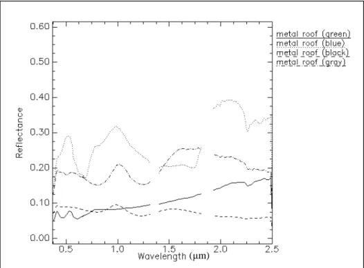
High spectral variability occurs in the field spectra of four metal roof samples collected from different sites (Figure 8). Not only is the intensity of reflectance, but also the spectral curves are significantly varied among them. Since these metal rooftops are lacquered, the surface reflectance from the coating is the dominant component of the signal. The metal roof with black coating has a more similar spectral curve to the metal

roof with gray coating than those with green color and blue color through visible to near-infrared range. The peaks of spectral curves in the visible region also correspond to the colors of the coatings.

According to the spectral signatures described above, most of the urban surface materials are lacking of consistent and strong absorption features (e.g., asphalt, water, metal). Even though some materials such as concrete have consistent spectral reflectance, their spectral signatures might still be contaminated by the surroundings. For instance, soil might introduce small absorption feature near 2.2µm into the spectral signatures. Furthermore, the similar materials might have very different spectral signatures (i.e., metal rooftops).

In summary, high spectral variability of the urban surface materials results from several reasons: (1) humanmade materials have an inconsistent mixture of ingredients; (2) natural materials such as rocks and gravels are comprised of different mineral compounds; (3) water bodies have various turbidity, suspended materials, and underwater backgrounds; (4) urban plants have individual growing and senescing conditions due to various irrigation and fertilization; (5) the reflectance spectra of target materials are sensitive to interactions with the environmental variables (e.g., soil, water). Consequently, most urban surface materials are not differentiable by matching the absorption bands. The full spectral mapping methods, such as spectral angle mapper, which compare the spectra with continuum shapes and/or very broad absorptions using the full wavelength range, are more feasible for mapping urban materials than other band-matching methods. In addition, the signature extension approach is less applicable for the spectroscopic analysis of urban surface materials. The need of a local spectral library for urban analysis, which provides a variety of reference spectra of desired targets and minimizes the effects of the spectral variability, is therefore verified.

Material Identification

Spectral Analysis Method

The selection of a spectral analysis strategy for discrimination of urban surface materials should correspond to the spectral characteristics and contextual situation of the urban surface materials being investigated. Based on the previous discussion of the spectral signatures of urban surface materials in the Park City region, the full spectral mapping approach was adopted for the sequential spectral analysis. While other methods were evaluated, they were deemed less appropriate for the situation and likely less effective than the full spectral mapping approach.

The full spectral mapping methods can be separated into two groups, spectral similarity searches and spectral detection maps (Mustard and Sunshine, 1999). Two algorithms have been developed to define the similarity between image spectra and reference spectra. The first is binary encoding, which is extremely computationally efficient because it encodes the spectra into a 2-bit scheme (Goetz et al., 1985). The second algorithm in the group of spectral similarity searches is spectral angle mapper which determines the spectral similarity between the reference spectrum and the image spectrum by calculating the “spectral angle” between the two spectra (Kruse et al., 1993). Both target spectrum and reference spectrum are regarded as vectors in a space with dimensionality equal to the number of bands. Smaller values of the angle between the vectors correspond to higher spectral similarity between two spectra. The calculation of the spectral angleinvolves taking the arccosine of the dot product of the spectra by applying the following equation (Kruse et al., 1993):

 

t * r

 

║t║ * ║r║

where t is the target spectrum and r is the reference spectrum. As a result, field and laboratory spectra can be directly compared to image spectra.

In comparing the algorithms of binary encoding and spectral angle mapper, binary encoding is a simpler method and computationally more efficient than spectral angle mapper. However, based on the 2-bit scheme, binary encoding will highly generalize small, but important differences, between the target spectrum and the reference spectra. Thus, only spectral angle mapper was utilized in this research.

The version of spectral angle mapper (SAM) in the ENVI 3.2 image processing software package was applied to identify the surface materials in the low-altitude AVIRIS data of the Park City urban area. Since SAM utilizes the full spectral range, the noisy bands severely affected by atmospheric absorption and the unreliable bands due to the overlap of grates on the spectrometers are excluded from the analysis. The field spectra of 16 representative surface materials were selected from the regional spectral library of Park City to provide the reference signatures (Table 2).

Results

In the SAM analysis, the threshold value used for the maximum angle between spectral vectors was first established at 0.05 radians and later empirically tuned for the rule images of each target. The pixel values in a rule image represent the spectral angle in radians. Lower spectral angles (darker pixels) indicate better spectral matches to the reference spectrum. Lastly, the contrast of each rule image was stretched to adjust the SAM rule thresholds to highlight those pixels with the greatest similarity to the reference spectra.

Orthophotography obtained in May, 2000 at 3000-4000 feet above the study area (6-inch pixel size), and the field spectra associated with the location information

were used as the references for accuracy assessment. Field checks were also conducted for some targets, such as the young sidewalk trees without an obvious canopy, when the spatial resolution and spectral resolution of the orthophotography were still too coarse to validate the results.

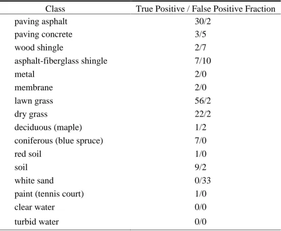
The accuracy assessment was conducted using a quantitative approach, which was applied to the individual abundance map derived from SAM. Since the SAM rule thresholds have been optimized and the contrast of each rule image has been stretched, all pixels with different levels of darkness appeared in each abundance map are regarded as a single class. There are 100 pixels randomly selected in the AVIRIS image of the study area. A mask with the location marks of these pixels is superimposed on each abundance map to check the agreement between each pixel’s class and its reference. Because not all pixels in the rule image are classified by SAM, only the pixels appeared in the abundance maps and also randomly selected are taken into account. A true positive / false positive fraction is used to indicate the classification accuracy of each abundance map, where the “true positive”means the number of pixels with the class agreed with the reference and the “false positive”represents the number of pixels with the class not agreed with the reference (Table 3).

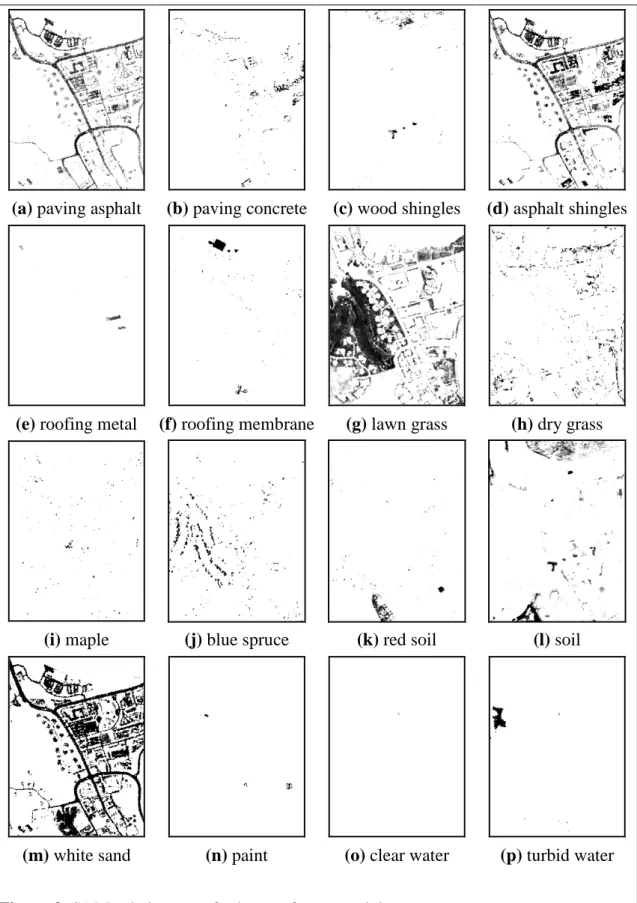
When 16 field spectra (endmembers) were processed via the SAM algorithm, 11 types of materials were successfully identified in the AVIRIS scene in that the true positive pixels outnumbered the false positive pixels (Figure 9, Table 3). For example, the linear features of roads were successfully identified in the AVIRIS data, and they were differentiated from water (Figure 9a); The SAM selectively identified the pixels of a particular metal roof, but did not identify the other metal roofs with high spectral variability (Figure 9e). These results confirm that the SAM analysis using field spectra as the reference is capable of discriminating many urban surface materials in the

low-altitude AVIRIS image. However, the paving concrete, the wood shingle, the asphalt-fiberglass shingle, the maple trees, and the white sand were not easily discriminated. Their false positive pixels outnumber true positive pixels (Table 3). A few sidewalks paved by concrete were identified in the abundance map. However, those sidewalks surrounded by trees and buildings were not identified due to the spectral mixture problem (Figure 9b). In addition, a few pixels of paving asphalt were misclassified as paving concrete because their spectral reflectance shapes were similar throughout the near-and mid-infrared region, even though they were apparently differentiable by the intensity of reflectance. The white sand and the paving asphalt were confused for the same reason (Figure 9a, 9m). These two cases reveal the drawback of SAM, which is insensitive to the difference in albedo. SAM did not discriminate the maple trees from the other deciduous trees (Figure 9i). However, SAM differentiated the blue spruce, the lawn grass, and the dry grass. The wood shingles were not differentiated from the senesced sagebrush (Figure 9c). The asphalt shingles and the paving asphalt were confused (Figure 9a, 9d). In these two cases, the confused materials are spectrally similar so that their differences are too subtle to be discriminated by SAM.

Summary

By comparing the field spectra in the study area, the results reveal that the absorption features of most urban surface materials are inconsistent. However, the spectral reflectance shapes of the field spectra still provide sufficient information for discriminating many different surface materials. Furthermore, the same material (e.g., asphalt, grass), under varying age and environmental conditions can be differentiated by comparing the spectral reflectance shapes. In some cases, the level of detail

differentiable by the field spectra is beyond conventional classification schemes. The great diversity and variability of field spectra suggest that the use of existing public spectral libraries is limited. Creation of a local spectral library is the best approach. In this study, the local spectral library for Park City serves as a prototype for development of other urban spectral libraries.

The spectra of most urban surface materials are characterized by their continuum shapes and/or very broad absorptions instead of diagnostic narrow absorptions. By linking the spectral characteristics of urban surface materials back to spectral analysis techniques, spectral angle mapper that uses the full spectral response was effective in this research. The results of the SAM confirm that a pixel-based analysis associated with field spectra as the reference is capable of identifying many urban surface materials in the low-altitude AVIRIS data. It is believed that additional materials such as paving concrete of small sidewalks can be extracted using the same method with higher spatial resolution.

In this study, several materials were not spectrally differentiable by SAM. Moreover, the size of the mapping area in the spectral analysis relates to the discriminability of the spectral analysis technique and the complexity of endmembers. When the discriminability of the technique is increased and/or the complexity of endmembers is decreased, the number of unclassified pixels is, likewise, increased. There is no single method universally feasible for extracting all urban surface materials. Consequently, a combination of different methods including the use of spatial information such as texture characteristics is required in the future to precisely extract all of the desired targets. It is necessary to aggregate the classification results derived from the various methods to meet the data requirements of specific applications, to expand the mapping area and to maximize the mapping accuracy simultaneously. Since

the errors existing in the maps of individual materials would be aggregated into the final product, it is important to verify the quality of individual material maps in advance.

The number and importance of urban applications, for which detailed compositional information on surface materials is essential, is growing. The relationship of these surface materials to non-point pollution retention, surface water runoff, and urban heat retention are a few applications which require high resolution spatial and compositional information collected over a large area. This study indicates that urban remote sensing at these levels of resolution can be accomplished.

References

Barrett, E. C. and L. F. Curtis (1992): Demography and Social Change, Introduction to Environmental Remote Sensing, London, Chapman & Hall, 363 p.

Clark, R. N. (1999): Chapter 1: Spectroscopy of rocks and minerals, and principles of spectroscopy, Manual of Remote Sensing, 3rded., John Wiley and Sons, Inc., New York, pp. 3-58.

Curran, P. J. (1994): Imaging spectrometry – Its present and future role in environmental research, Imaging Spectrometry –a Tool for Environmental Observations, ECSC, EEC, EAEC, Brussels and Luxembourg, Netherlands, pp. 1-23.

Goetz, A. H. F., G. Vane, J. E. Soloman, and B. N. Rock (1985): Imaging spectrometry for Earth remote sensing, Science, 228(4704): 1147-1153.

integration of AVIRIS and IFSAR for urban analysis, Photogrammetric Engineering and Remote Sensing, 64: 813-820.

Hunt, G. R. (1977): Spectral signatures of particulate minerals in the visible and near infrared, Geophysics, 42(3):501-513.

Hunt, G. R. (1979): Near-frared (1.3-2.4µm) spectra of alteration minerals –potential for use in remote sensing, Geophysics, 44(12): 1974-1986.

International Geosphere-Biosphere Program (1995): Land Use and Land Cover Change - Science Research Plan, IGBP rpt. 35, IGBP, Stockholm.

Jensen, J. R., and D. C. Cowen (1999): Remote sensing of urban/suburban infrastructure and socio-economic attributes, Photogrammetric Engineering & Remote Sensing, 65(5): 611-622.

Kruse, F. A., A. B. Lekhoff, and J. B. Dietz (1993): Expert system-based mineral mapping in northern Death Valley, California/Nevada, using the airborne visible/infrared imaging spectrometer (AVIRIS), Remote Sensing of Environment, 44: 309-336.

Microsoft (2001): Microsoft Encarta Encyclopedia Deluxe, CD software, Microsoft Corporation.

investigations using remote sensing data, Manual of Remote Sensing, 3rd ed., John Wiley and Sons, Inc., New York, pp. 251-306.

Ridd, M. K., N. D. Ritter, N. A. Bryant, and R. O. Green (1992): AVIRIS data and neural networks applied to an urban ecosystem, Third Airborne Geoscience Workshop, National Aeronautics and Space Administration, Jet Propulsion Laboratory, Pasadena, CA., 1: 129-131.

Ridd, M.K. (1995): Exploring the VIS Model for Urban Ecosystems Analysis Through Remote Sensing, International Journal of Remote Sensing, 16(12):2165-2186.

Rockwell, B. W., R. N. Clark, K. E. Livo, R. R. McDougal, R. Kokaly, and J. S. Vance (1999): Preliminary materials mapping in the Park City region for the Utah USGS-EPA Imaging Spectroscopy Project using both high and low altitude AVIRIS data, Summaries of the Eighth JPL Airborne Earth Science Workshop, Jet Propulsion Laboratory, Pasadena, CA., pp. 365-376.

Rockwell, B. W. (2000): AVIRIS data calibration information in Park City region, USGS Spectroscopy Lab, URL:

http://speclab.cr.usgs.gov/earth.studies/Utah-1/park_city_calibration.html (last date accessed: 15 June 2001).

N

(a)

(b) (c)

Figure 1. AVIRIS scenes of the Park City, Utah. (a) high-altitude AVIRIS scene showing white box that outlines the study area where both covered by the high- and low-altitude AVIRIS overflights. (b) high-altitude AVIRIS scene with the white arrow indicating the rooftop of the supermarket (resampled to match the low-altitude AVIRIS coverage). (c) low-altitude AVIRIS scene.

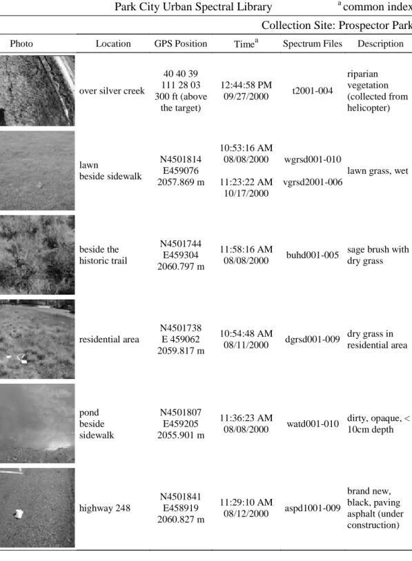
Table 1. Data Format of the Urban Spectral Library

Park City Urban Spectral Library acommon index

Collection Site: Prospector Park

Photo Location GPS Position Timea Spectrum Files Description

over silver creek

40 40 39 111 28 03 300 ft (above the target) 12:44:58 PM 09/27/2000 t2001-004 riparian vegetation (collected from helicopter) lawn beside sidewalk N4501814 E459076 2057.869 m 10:53:16 AM 08/08/2000 11:23:22 AM 10/17/2000 wgrsd001-010 vgrsd2001-006

lawn grass, wet

beside the historic trail N4501744 E459304 2060.797 m 11:58:16 AM 08/08/2000 buhd001-005

sage brush with dry grass residential area N4501738 E 459062 2059.817 m 10:54:48 AM 08/11/2000 dgrsd001-009 dry grass in residential area pond beside sidewalk N4501807 E459205 2055.901 m 11:36:23 AM 08/08/2000 watd001-010 dirty, opaque, < 10cm depth highway 248 N4501841 E458919 2060.827 m 11:29:10 AM 08/12/2000 aspd1001-009 brand new, black, paving asphalt (under construction)

Figure 3. Reflectance spectra of three concrete.

Figure 2. Reflectance spectra of concrete, sand, gravel, and calcite.

(μm)

Figure 4. Reflectance of three asphalt samples in different weathered conditions.

Figure 5. Reflectance spectra of the vegetation in summer.

(μm)

Figure 6. Reflectance spectra of the vegetation in autumn.

Figure 7. Reflectance spectra of four water samples.

(μm)

Table 2. Reference Spectra Provided by the Urban Spectral Library

Category Field Spectra

I. Paving Materials 1.1 paving asphalt 1.2 paving concrete

II. Roofing Materials 2.1 wood shingle

2.2 asphalt-fiberglass shingle 2.3 metal

2.4 membrane

III. Vegetation 3.1 lawn grass 3.2 dry grass

3.3 deciduous (maple) 3.4 coniferous (blue spruce)

IV. Others 4.1 red soil 4.2 soil

4.3 white sand

4.4 paint (tennis court) 4.5 clear water

4.6 turbid water Figure 8. Reflectance spectra of four metal roofs.

Table 3. The Accuracy Assessment of the Material Abundance Maps Class True Positive / False Positive Fraction

paving asphalt 30/2 paving concrete 3/5 wood shingle 2/7 asphalt-fiberglass shingle 7/10 metal 2/0 membrane 2/0 lawn grass 56/2 dry grass 22/2 deciduous (maple) 1/2

coniferous (blue spruce) 7/0

red soil 1/0

soil 9/2

white sand 0/33

paint (tennis court) 1/0

clear water 0/0

(a) paving asphalt (b) paving concrete (c) wood shingles (d) asphalt shingles

(e) roofing metal (f) roofing membrane (g) lawn grass (h) dry grass

(i) maple (j) blue spruce (k) red soil (l) soil

(m) white sand (n) paint (o) clear water (p) turbid water