聲譽與公平動機在自願捐獻機制中對實驗對象合作行為影響的實驗研究

行政院國家科學委員會專題研究計畫 成果報告

聲譽與公平動機在自願捐獻機制中對實驗對象合作行為影

響的實驗研究

中 華 民 國 94 年 4 月 28 日

Fairness and Strategies in Simple Public Goods Experiments

Li-Chen Hsu and Yusen Sung

Abstract: We conduct experiments on three threshold public good provision games (simultaneous game, sequential game, and dictator game) to examine the effects of fairness and strategies on contributions. Our data show that game predictions cannot explain contribution behavior. In addition, only players in the simultaneous game contribute fairly. The first players in the sequential game and the dictators in the dictator game choose to free ride on their partners. These findings indicate that players contribute fairly not because of fairness concern. Once bargaining power provides them an opportunity to free ride, they will do so. However, since complete free-riding cannot be observed in the dictator game, strategies concern alone is insufficient to explain the contribution behavior, either.

Keywords: Experiments, Simultaneous game, Sequential game, Dictator game

JEL Classification: C92, H41 摘要：我們操作三種有門檻的公共財提供賽局 (同時行動賽局，相繼行動賽局，與獨裁 者賽局)，以檢驗公平與策略動機對捐獻行為的影響。我們的實驗證據顯示，賽局的理 論預期無法解釋捐獻行為。另外，只有同時行動賽局中的參賽者採取公平的捐獻。相繼 行動賽局中的先行動者與獨裁者賽局中的獨裁者都選擇免費乘車策略。這些發現顯示， 參賽者採取公平的捐獻並非他們存有公平的意念，而是他們居於同等地位。一旦他們被 賦予較強的協商力量，則會採取盡可能由對方捐獻的策略。不過由於我們在獨裁者賽局 中並未觀察到獨裁者令接受者捐出所有的稟賦，策略的動機亦不足以單獨解釋捐獻行 為。 關鍵詞：實驗，同時行動賽局，相繼行動賽局，獨裁者賽局 JEL 分類: C91, H41

1. INTRODUCTION

Experimental studies have constantly found cooperative behavior in non-cooperative games. For instance, in a linear public provision game the dominant-strategy Nash equilibrium is complete free-riding. However, related experimental studies often find high contributions, sometimes around 40% to 60% of the subjects’ endowments. Furthermore, though the levels of contributions decay over trials, the dominant-strategy Nash equilibrium never shows up.1

Similar cooperative outcomes can be observed in the ultimatum game. In the ultimatum game the proposer proposes a division of $Q between himself and the responder. If the responder agrees with the proposer’s proposal, then each party obtains the amount of money that the proposer suggests. Otherwise, each player gets zero. If both players pursue maximum monetary rewards, then the subgame perfect equilibrium suggests that the proposer will propose a miniature amount of money to the responder. Since this offer is better than nothing, the responder can only accept it.

Again, experimental findings on ultimatum games differ largely from the subgame perfect equilibrium. In non-repeated ultimatum games, Güth, Schmittberger, and Schwarze (1982), Forsythe et al. (1994), and Roth et al. (1991) find that the proposer often offers 40% of $Q to the responder, much higher than what the subgame perfect equilibrium predicts. This result suggests that the proposer do not behave selfishly, but intend to share $Q with the responder equally (or near equally). Furthermore, experimental evidence shows that offering less than 20% of $Q to the responder is often rejected.2

A large number of experimental studies have investigated the motives behind the cooperative behavior in the public good provision game and ultimatum game. Fairness is one of the concerns that have attracted a broad discussion to date. For intstance, Pranikar and Roth (1992) compare the experimental results of ultimatum game and best-shot game. They find that in the ultimatum game the proposers generally offer around 40 percent of the

1

See for instance Marewll and Ames (1981), Andreoni (1988), and the surveys by Davis and Holt (1993) and Kagel and Roth (1995).

2

Experimental results from multi-period and repeated ultimatum games are also inconsistent with the game prediction. One can refer to Ochs and Roth (1989) for the former game and Prasnikar and Roth (1992) for the latter design. For more related studies, one can refer to the surveys by Güth and Teitz (1990) and Camerer and Thaler (1995).

pie to the responder in all ten trials. In the best-shot game, no matter full or partial information, first movers’ offers consistently converge to zero, with a quicker decay with full information. Pranikar and Roth therefore conclude that if sharing the burden of providing the public good is impossible, then fairness consideration cannot be applied.

Forsythe et al. (1994) compare the experimental results from the ultimatum game and dictator game. Under each game the pay and on-pay conditions are conducted. Their idea is that if fairness alone is able to explain the deviation of subgame perfect equilibrium in the ultimatum game, then the distributions of offers should be the same in the ultimatum game and dictator game. They find in games with pay that the distributions of offers different significantly between the two games, against the fairness hypothesis. However, in games without pay, the difference is insignificant.

In public good provision experiments, Andreoni, Brown, and Vesterlund (2002) ask whether the opportunities to play fairly matter, besides the intensions of playing fairly. They conduct three two-person public goods games: simultaneous game, sequential game, and best-shot game. In all three games, only one person contributes in Nash equilibrium, but different choices by subjects are found. Specifically, the average contributions for two players are almost identical for every round in the simultaneous game. In the sequential game, giving by player two is higher than that by player one, but the difference is statistically insignificant. These results differ from what the equilibrium predicts. However, in the last five rounds of the best-shot game, more than sixty percent of the subjects’ choices conform to the predicted outcome. The reason is simply that the first mover in the best-shot game has no opportunity to play fairly.

In this paper we seek to explore the fairness and strategies hypotheses in a two-player threshold public good provision game. Three types of games are considered: simultaneous game, sequential game, and dictator game. The threshold public goods game has several merits as compared with the public provision game without a threshold: First, the threshold provides the players a focal point associated with fair contribution. It is reasonable to assume that the fair contribution is for both players to share the threshold equally. However, the public good provision game without a threshold lacks this focal point. Second, besides the complete free-riding Nash equilibrium observed in the public good provision game

without a threshold, the threshold public good game has another Nash equilibria, the threshold Nash equilibria. Since the complete free-riding Nash equilibrium is generally not observed in experimental studies, the threshold Nash equilibria provide us another theoretical solution to test. Third, the threshold design in the sequential game makes the public good provision game similar to the ultimatum game. Therefore, we can also compare our results with those from ultimatum games.

The rest of the paper is organized as follows. Section 2 provides a simple model and the experimental design. Experimental results are reported in Section 3. Section 4 concludes.

2. EXPERIMENTAL DESIGN

2.1. The Model

We explore the effect of fairness and strategies on the provision of public goods in three two-person threshold public goods games. In the first game player 1 and player 2 make their contributions simultaneously. We call this game the simultaneous game and denote it briefly as simu. In the second game player 1 moves first. After observing player 1’s contribution, player 2 makes her decision. This game is indicated as the sequential game and is denoted as seq. The third game is the dictator game, in which player 1 makes not only her own contribution decision, but also player 2’s. The dictator game is abbreviated as

dic.

Two players in a group provide the public good. Each player is endowed with an exogenous income w. Denote x as consumption of a private good by individual i and i g i

as i’s contribution to the public good. Each player faces a budget constraint x_i +g_i =w. Since in the threshold public goods game the motive of fear may prevent individuals from contributing, a refund is imposed if total contributions fail to meet the threshold. However, any contributions beyond the threshold are not returned. That is, the motive of greed (or free-riding) still remains. The individual’s utility function is written as u_i = x_i +G+r_i, where G is the public good and r is the refund. If the sum of contributions reach a certain i

Two different levels of threshold are adopted in each game. In the low-threshold condition T =w such that the public good can be provided by one player alone. In the high-threshold condition w<T <2w, so the public good must be provided by both players together. Nash equilibria in the three games depend on the levels of threshold. Let us start with the low-threshold condition. In the simultaneous game, the best response to g_−i =0 is 0g_i = or g_i = for i = 1, 2. Thus, we first have two Nash equilibria: In one w

equilibrium both players adopt a complete free-riding strategy and in the other equilibrium one player contributes nothing and the other player contributes everything. Besides the two equilibria, it is obvious that any contributions such that the sum of g1 and g2 equals T are also Nash equilibria. We call these equilibria the threshold Nash equilibria. In the sequential game, player 2 is better off if he gives less than w and if the public good is provided. Therefore, the subgame perfect Nash equilibrium is that player 1 gives ε in the first stage and lets player 2 fill up the gap by giving w−ε in the second stage. Finally, since in the dictator game player 1 makes decisions for both players, he will contribute nothing and make player 2 give w.

Nash equilibria vary slightly in the high-threshold condition. Since now the public good cannot be provided by only one player, in the simultaneous game the best response to

0 = −i

g is g_i =0. Besides the complete free-riding Nash equilibrium, it remains that any contributions such that g1+g2 =T are also Nash equilibria. In the sequential game since

player 2 is better off as long as the public good is provided, the subgame perfect Nash equilibrium is that player 1 gives T−w in stage 1 and leave player 2 to give w in stage 2. Finally, it is obvious that in the dictator game the equilibrium is the same as that in the sequential game.

2.2. Experimental Parameters

As was described above, there are two conditions associated with different levels of threshold and there are three games in each condition. We conducted one session for each game in each condition, for a total of six sessions. We recruited 40 subjects in each session from intermediate economic classes at National Chengchi University and National Taiwan

University. The framework of the experiment is illustrated in Table 1. None of the subjects had ever participated in any public goods experiments. In each session subjects were randomly and anonymously assigned to groups of two and played the game for 10 rounds.

In each session of the simultaneous-move game and sequential game, 20 subjects were assigned the role of player 1 and were placed in the same room. In the other room another 20 subjects were assigned the role of player 2. Subjects were randomly re-matched starting each new round, but their identities remained unchanged across all ten rounds. In each session of the dictator game, 40 subjects were also divided equally between two rooms. Since player 2 in the dictator game did not make any decisions, different from the other two games, all of the 40 subjects were assigned the role of player 1 but they were informed that subjects in the other rooms were player 2. To consider the anonymity effect proposed by Bolton and Zwick (1995), subjects were asked to put their decisions and calculate the payoffs for both players on two copies of the decision form. One copy was for their record, and the other copy was for the recipients, though they were not aware that the recipients were actually absent. They then turned in the copy for the recipients to assistants with the front side facing down so that anyone in the room, except themselves, would not notice their decisions.

Subjects were given written instructions, which the experimenter read over with the subjects. Before playing the games, the experimenter gave a quiz, asking subjects to calculate the payoffs in three specific examples. None of the subjects answered all three questions wrong.3

In each session of the experiment, subjects are each endowed with $20 per round and are instructed to invest this endowment between object X (the private good) and object Y (the public good). $1 invested in X will earn the subject $1. In the low-threshold condition, if group investment in Y reaches $20, then each member will earn $20 from Y. In the

3

Subject #21 in SimuT>w answered question 2 incorrectly. Subjects #8 and #9 in SeqT>w answered question 1 incorrectly. In SeqT>w, subjects #20 and #27 answered question 1 incorrectly and #26 and #27 answered question 2 incorrectly. In DicT=w, subjects #4 and #15 answered question 1 incorrectly and #3, #27 and #34 answered question 3 incorrectly. In DicT>w, subjects #4, #8, and #30 answered question 1 incorrectly and #8 and #38 answered question 2 incorrectly.

high-threshold condition, if group investment in Y reaches $30, then each member will earn $30 from Y. In both conditions if group investment in Y fails to meet the threshold, then the money invested in Y will be returned to individual subjects and will be invested in X instead, which will earn the subjects dollar for dollar.

In the following section, we will explore how well the data conform to the game predictions. In addition, we will investigate whether fairness or strategies explains the contribution behavior better. Since a threshold is imposed in the experiments, it is reasonably to assume that the fair contribution is T/2. Therefore, if fairness alone can explain contribution behavior, then we should observe subjects contributing T/2, regardless of the types of game and the levels of threshold. If significant differences occur across various experiments, then strategies or other motives must also play a role.

3. RESULTS

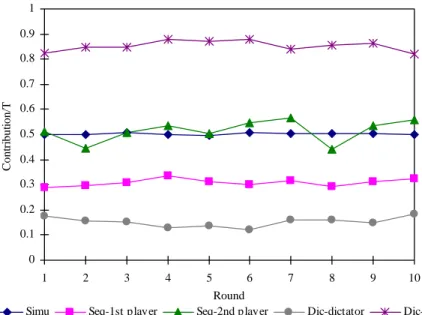
We will first explore the differences between the high- and low-threshold conditions and then will compare the differences between different types of games. Since the levels of threshold in two conditions differ, it is reasonable to expect that significantly higher levels of contributions will occur in the high-threshold condition than in the low-threshold condition. Actually this is also shown by our data. Therefore, instead of using the levels of contributions in various experiments, we compare the ratios of contributions to threshold. The preliminary results are illustrated in Table 2 and Figures 1 and 2.

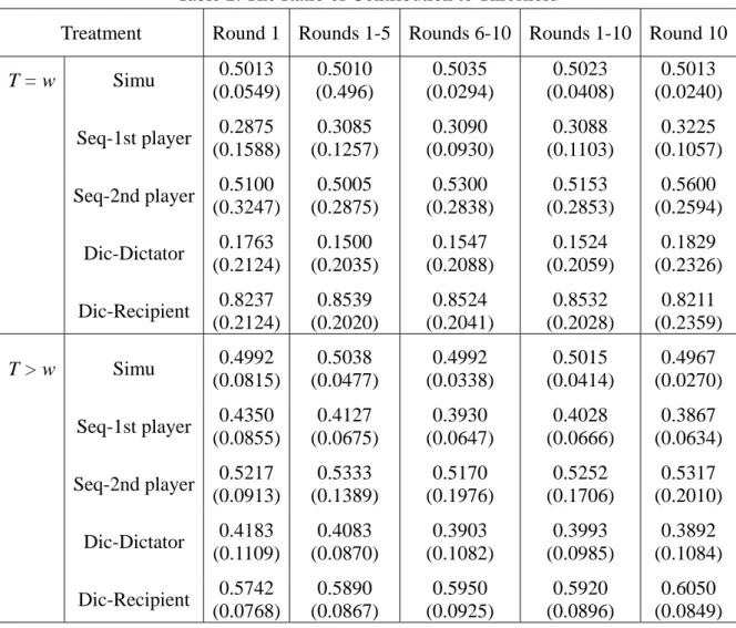
Several observations can be noticed directly. First, the ratios of contributions to threshold are more diverse in the low-threshold condition than in the high-threshold condition. In the high-threshold condition subjects of different roles generally share 40% to 60% of the threshold. By contrast, in the low-threshold condition recipients in the dictator game share more than 80% of the threshold and the first players in the sequential game generally share only 30% of the threshold. The dictators in the dictator game share even lower, only about 15% of the threshold on average.

Second, there is no decay in all experiments. In addition, except the second players in the sequential game, the contributions made by all other roles are smooth across all ten rounds. Third, the recipients in the dictator game are forced to contribute the most under

both conditions. By contrast, the dictators in the dictator game and the first players in the sequential game seem the greediest ones. However, on average complete free riding (that is, contributing zero in the low-threshold condition and one-third of the threshold in the high-threshold condition) never show up. The last thing to observe is that players in the simultaneous game and the second players in the sequential game seem to play fairly. In both conditions, players in the simultaneous game generally share about 50% of the threshold with the other group members. The second players in the sequential game behave similarly, with contributing slightly higher.

These observations give us a first insight that only players in the simultaneous game and the second players in the sequential game adopt fair strategy. Dictators in the dictator game and the first players in the sequential game free ride most as compared to other roles. However, even though they have the power to free ride, they do not always behave this way. On average complete free riding (that is, contributing zero in the low-threshold condition and one-third of the threshold in the high-threshold condition) never show up.

In the following subsection we will investigate how well the data conform to the game predictions. In Subsection 3.2 and 3.3 we will explore the differences across various games and the differences between the two conditions.

3.1. Comparing the Data with Game Predictions

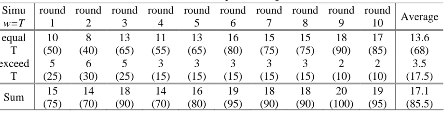
Let us start looking at the data from simultaneous experiments. Looking at the individual data, we find that no one contributes zero in any round under both conditions. Therefore, the complete free-riding Nash equilibrium never shows up. From Table 2, we can see that on average players generally contribute half of the threshold in both conditions. Therefore, we may ask how often the threshold Nash equilibrium appears. Table 3 reports the numbers and percentages of groups reaching the threshold in various experiments. It can be seen that the numbers of groups reaching the threshold are very close in both conditions: Three-fourths of the groups successfully provide the public good in the first round. This magnitude increases over rounds and in the final rounds 95% of the groups reach the threshold under both conditions, with an average of about 85% over all 10 rounds.

condition than in the low-threshold condition. Threshold Nash equilibria occur in 50% of the groups in the low-threshold condition in the first round, but only in 30% of the groups in the high-threshold condition. Though in the final round these magnitudes are 85% in the low-threshold condition and 90% in the high-threshold condition, most of the time the latter condition reveals more wastes. On average, the threshold Nash equilibria occurs 68% of the groups in the low-threshold condition and 56% of the groups in the high-threshold condition. Therefore, the data generated from the simultaneous game do not conform to the game predictions very well.

We now look at the sequential-move game. Nash equilibria predict that player 1 in the low-threshold condition should give a tiny amount of money ($1 in our experiments) and in the high-threshold condition should give $10. Player 2 is left to fill up the threshold. Looking at the individual data, we find that 4 out of 20 first players in the low-threshold condition contribute $1 in the first round. In round 4 through round 10 only one first player gives $1 in round 8, contradicting the game prediction. On the other hand, in the high-threshold condition a number of player ones do contribute only $10. For instance, 3 out of 20 or 15% of player ones do so in the first round and in the final round this magnitude rises to 40%. However, these magnitudes are still far below the game prediction.

Next let us ask how often the threshold Nash equilibria occur. Table 3 shows that on average 72% of the groups in the low-threshold condition and 83.5% of the groups in the high-threshold condition provide the public good successfully. In both conditions, only one group in one round over contributes. These results, along with the complete free-riding result above, suggest that higher threshold gives first players more bargaining power. In the high-threshold condition first players must give at least $10 if they are willing to provide the public good. Having given one-third of the threshold provides them the bargaining power, preventing them from giving more. As a result, the second players in the high-threshold condition are more willing to give all than do the second players in the low-threshold condition.

Finally, the theory predicts that in the dictator game dictators will give zero in the low-threshold condition and $10 in the high-threshold condition. Again, our data from the dictator experiments conform little to game predictions. In the low-threshold condition,

only 16 (out of 38) players give zero and 9 players give $10 in the first round, with an average giving of $3.5. Even in the final round, there are only 17 players give $0, but 10 players give $10 and one player gives even as large as $15. On the other hand, in the high-threshold condition, only 10 (out of 40) players give $10 and as high as 19 players give $15 or more in the first round. In the final round, more (17) players give $10, but there are still 8 players give at least $15. All of these results contradict the game predictions.

Investigating whether the threshold is reached in the dictator game is the other way to examine the game predictions. Table 3 shows that except in round 4, the public good is successfully provided in every group in the low-threshold condition. However, over contributions occur on average 1.4% of the time and this outcome can hardly be explained. Efficient public good provision appears even lower in the high-threshold condition, with an average of only 89.5% of the time. The public good fails to be provided 1.9% of the time and wasteful contributions occur 2.3% of the time on average. All of these observations cannot be explained by game predictions.

3.2. Comparing the Contributions in Various Games within the Same Condition

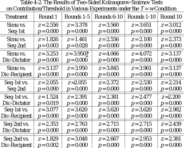
As can be observed from Figure 1, in the low-threshold condition players in the simultaneous game and the second players in the sequential game make similar contributions, about half of the threshold. However, as reported in Table 4-1 and Table 4-2, a two-sided Mann-Whitney U test show that these two roles make the same contribution in the first five rounds, but the second players in the sequential game make significantly higher contributions than do the players in the simultaneous game in the last five rounds. A two-sided Kolmogorov-Smirnov test shows that contributions made by these two roles are significantly different in all 10 rounds. We also observe that recipients in the dictator game make significantly more contributions than all other roles. By contrast, the least contributions are made by dictators, followed by the first players in the sequential game.

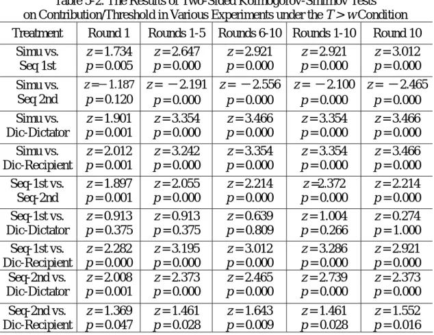
Now let us turn to the high-threshold condition. Tables 5-1 and 5-2 report the statistical results. Again, players in the simultaneous game and the second players in the sequential game give about half of the threshold to the public good, with giving by the latter significantly higher than giving by the former. Also similar to the finding in the

low-threshold condition, recipients give significantly more than all other roles do, but contributions made by dictators and the first players in the sequential game do not differ significantly. These results suggest that as the threshold increases, the first players in the sequential game behave more like dictators.

3.3. Comparing the Contributions within the Same Game but across Different Conditions

Tables 6-1 and 6-2 report the statistical results associated with the ratios of contribution to threshold within the same game but across the two conditions. It can be observed that contributions made by players in the simultaneous game and the second players in the sequential game do not differ between the high threshold and the low threshold conditions. The first players in the sequential game and the dictators make significantly more contributions to meet the threshold in the high-threshold condition than in the low-threshold condition. By contrast, the ratios of contribution to threshold for recipients in the dictator game are significantly lower in the high-threshold condition than in the low-threshold condition.

Since the first players in the sequential game and the dictators are forced to make at least $10 (or one-third of the threshold) in the high-threshold condition if they are willing to provide the public good but they can give nothing in the low-threshold condition, it may be meaningless to compare the ratios of contribution to threshold of these two roles. We therefore ask how generous they are; namely, besides the necessary contributions, how much more money they give under the two conditions. We measure the generosity under the high-threshold condition by using (contribution/threshold－1/3) and under the low-threshold condition simply by using contribution/threshold. A two-sided Mann-Whitney U test show that the first players in the sequential game give significantly more extra money to the public good under the low-threshold condition than under the high-threshold condition. By contrast, the amounts of extra money contributed by dictators under the two conditions do not differ significantly. Again, this verifies a previous result that the first players in the high threshold tend to free ride more.

4. CONCLUSION

We conduct experiments on three threshold public good provision games: the simultaneous game, the sequential game, and the dictator game. Two levels of threshold are applied to each game. Our data show that game predictions cannot explain contribution behavior in all three games. Specifically, in the simultaneous game the complete free-riding Nash equilibrium never shows up. The other equilibria, the threshold Nash equilibria, occur in 68% of the groups in the low-threshold condition and in only 56% of the groups in the high-threshold condition. These results contradict the game predictions that contribution behavior should conform to either type of equilibria. The data from the sequential game are way below the game predictions as well. In the last seven rounds of the low-threshold condition, only one player one contributes $1 as the theory predicts. In the high-threshold condition only 15% of player ones give $10 in the first round. Thought this magnitude rises to 40% in the final round, it is still far below the game prediction. The results from the dictator game can even hardly be explained by the game predictions. In the final round of the low-threshold condition, only 17out of 38 players give $0. On the other hand, in the final round of the high-threshold condition, only 17 out of 40 players give $10.

Findings from our experiments cannot be explained by fairness alone. Our data show that players contribute fairly only in the simultaneous game, in which both group members have equal bargaining power. In the sequential game, the first players in the low-threshold condition share only 30% of the threshold on average. Though this magnitude increases to about 40% in the high-threshold condition, it is still far below the fair share (50%). These outcomes indicate players in the simultaneous game play fairly not because they intend to, but because they have equal position. Once players are endowed with more bargaining power, they tend not to share the contributions fairly.

However, strategies cannot explain the data, either. Our data show that player ones in the sequential game do not choose the complete free-riding strategy, suggesting that they have strategies concern in mind, since player twos may revenge by letting the public good fail to be provided. However, if strategies concerns fail to explain the results from the dictator game, in which the theory predicts that dictators should allocate all of the recipients’ endowments the public good. Unfortunately, this cannot be observed from our data.

Table 1. The Framework of the Experiment

Simultaneous move

Sequential

move Dictator

w = T 40 subjects 40 subjects 38 subjects*

w < T 40 subjects 40 subjects 40 subjects *: In the dictator game with T = w, subject #29 continuously put wrong payoffs in every round except round 1. Subject #38 did not put any words on the decision form in round 4. The data related to these two subjects are excluded from the sample.

Table 2. The Ratio of Contribution to Threshold

Treatment Round 1 Rounds 1-5 Rounds 6-10 Rounds 1-10 Round 10

T = w Simu 0.5013 (0.0549) 0.5010 (0.496) 0.5035 (0.0294) 0.5023 (0.0408) 0.5013 (0.0240) Seq-1st player 0.2875 (0.1588) 0.3085 (0.1257) 0.3090 (0.0930) 0.3088 (0.1103) 0.3225 (0.1057) Seq-2nd player 0.5100 (0.3247) 0.5005 (0.2875) 0.5300 (0.2838) 0.5153 (0.2853) 0.5600 (0.2594) Dic-Dictator 0.1763 (0.2124) 0.1500 (0.2035) 0.1547 (0.2088) 0.1524 (0.2059) 0.1829 (0.2326) Dic-Recipient 0.8237 (0.2124) 0.8539 (0.2020) 0.8524 (0.2041) 0.8532 (0.2028) 0.8211 (0.2359) T > w Simu 0.4992 (0.0815) 0.5038 (0.0477) 0.4992 (0.0338) 0.5015 (0.0414) 0.4967 (0.0270) Seq-1st player 0.4350 (0.0855) 0.4127 (0.0675) 0.3930 (0.0647) 0.4028 (0.0666) 0.3867 (0.0634) Seq-2nd player 0.5217 (0.0913) 0.5333 (0.1389) 0.5170 (0.1976) 0.5252 (0.1706) 0.5317 (0.2010) Dic-Dictator 0.4183 (0.1109) 0.4083 (0.0870) 0.3903 (0.1082) 0.3993 (0.0985) 0.3892 (0.1084) Dic-Recipient 0.5742 (0.0768) 0.5890 (0.0867) 0.5950 (0.0925) 0.5920 (0.0896) 0.6050 (0.0849) Note: Standard deviations are in parentheses.

Table 3. The Number of Groups Reaching the Threshold Simu w=T round 1 round 2 round 3 round 4 round 5 round 6 round 7 round 8 round 9 round 10 Average equal T 10 (50) 8 (40) 13 (65) 11 (55) 13 (65) 16 (80) 15 (75) 15 (75) 18 (90) 17 (85) 13.6 (68) exceed T 5 (25) 6 (30) 5 (25) 3 (15) 3 (15) 3 (15) 3 (15) 3 (15) 2 (10) 2 (10) 3.5 (17.5) Sum 15 (75) 14 (70) 18 (90) 14 (70) 16 (80) 19 (95) 18 (90) 18 (90) 20 (100) 19 (95) 17.1 (85.5) Note: The total number of groups is 20. Percentages are in parentheses.

Simu w<T round 1 round 2 round 3 round 4 round 5 round 6 round 7 round 8 round 9 round 10 Average equal T 6 (30) 4 (20) 7 (35) 10 (50) 10 (50) 11 (55) 14 (70) 15 (75) 16 (80) 18 (90) 11.1 (55.5) exceed T 9 (45) 11 (55) 7 (35) 8 (40) 8 (40) 5 (25) 3 (15) 4 (20) 2 (10) 1 (5) 5.8 (29) Sum 15 (75) 15 (75) 14 (70) 18 (90) 18 (90) 16 (80) 17 (85) 19 (95) 18 (90) 19 (95) 16.9 (84.5) Note: The total number of groups is 20. Percentages are in parentheses.

Seq w=T round 1 round 2 round 3 round 4 round 5 round 6 round 7 round 8 round 9 round 10 Average equal T 15 (75) 13 (65) 14 (70) 15 (75) 15 (75) 15 (75) 16 (80) 12 (60) 14 (70) 14 (70) 14.3 (71.5) exceed T 0 (0) 0 (0) 0 (0) 0 (0) 0 (0) 0 (0) 0 (0) 0 (0) 1 (5) 0 (0) 0.1 (0.5) Sum 15 (75) 13 (65) 14 (70) 15 (75) 15 (75) 15 (75) 16 (80) 12 (60) 15 (75) 14 (70) 14.4 (72) Note: The total number of groups is 20. Percentages are in parentheses.

Seq w<T round 1 round 2 round 3 round 4 round 5 round 6 round 7 round 8 round 9 round 10 Average equal T 17 (85) 19 (95) 16 (80) 16 (80) 17 (85) 16 (80) 17 (85) 16 (80) 15 (75) 17 (85) 16.6 (83) exceed T 1 (5) 0 (0) 0 (0) 0 (0) 0 (0) 0 (0) 0 (0) 0 (0) 0 (0) 0 (0) 0.1 (0.5) Sum 18 (90) 19 (95) 16 (80) 16 (80) 17 (85) 16 (80) 17 (85) 16 (80) 15 (75) 17 (85) 16.7 (83.5) Note: The total number of groups is 20. Percentages are in parentheses.

Dic w=T round 1 round 2 round 3 Round 4 round 5 round 6 round 7 round 8 round 9 round 10 Average equal T 38 (100) 37 (97) 37 (97) 36 (95) 36 (95) 36 (95) 38 (100) 36 (95) 35 (92) 36 (95) 36.5 (96.1) exceed T 0 (0) 1 (2.6) 1 (2.6) 1 (2.6) 2 (5.3) 2 (5.3) 0 (0) 2 (5.3) 3 (7.9) 2 (5.3) 1.4 (3.7) Sum 38 (100) 38 (100) 38 (100) 37 (97.4) 38 (100) 38 (100) 38 (100) 38 (100) 38 (100) 38 (100) 37.9 (99.7) Note: The total number of groups is 38. Percentages are in parentheses.

Dic w<T round 1 round 2 round 3 round 4 round 5 round 6 round 7 round 8 round 9 round 10 Average equal T 35 (88) 36 (90) 37 (93) 34 (85) 36 (90) 37 (93) 35 (88) 35 (88) 37 (93) 36 (90) 35.8 (89.5) exceed T 3 (7.5) 3 (7.5) 2 (5) 4 (10) 1 (2.5) 2 (5) 2 (5) 3 (7.5) 1 (2.5) 2 (5) 2.3 (5.8) Sum 38 (95) 39 (98) 39 (98) 38 (95) 37 (93) 39 (98) 37 (93) 38 (95) 38 (95) 38 (95) 38.1 (95.3) Note: The total number of groups is 40. Percentages are in parentheses.

Table 4-1. The Results of Two-Sided Mann-Whitney U Tests

on Contribution/Threshold in Various Experiments under the T = w Condition Treatment Round 1 Rounds 1-5 Rounds 6-10 Rounds 1-10 Round 10

Simu vs. Seq 1st z = 5.490 p = 0.000 z = 6.276 p = 0.000 z = 6.653 p = 0.000 z = 6.382 p = 0.000 z = 6.362 p = 0.000 Simu vs. Seq 2nd z =－2.401 p = 0.016 z = －0.573 p = 0.567 z = －3.231 p = 0.001 z = －3.200 p = 0.001 z = －4.040 p = 0.000 Simu vs. Dic-Dictator z = 6.032 p = 0.000 z = 7.087? p = 0.000 z = 7.451 p = 0.000 z = 7.349 p = 0.000 z = 5.979 p = 0.000 Simu vs. Dic-Recipient z = 6.122 p = 0.000 z = 7.031 p = 0.000 z = 7.321 p = 0.000 z = 7.187 p = 0.000 z = 5.866 p = 0.000 Seq-1st vs. Seq-2nd z =－2.636 p = 0.008 z = －4.078 p = 0.000 z = －3.792 p = 0.000 z = －3.980 p = 0.000 z =－ 3.684 p = 0.000 Seq-1st vs. Dic-Dictator z = 2.320 p = 0.020 z = 3.774 p = 0.000 z = 3.149 p = 0.002 z = 3.375 p = 0.001 z = 2.487 p = 0.013 Seq-1st vs. Dic-Recipient z = 6.095 p = 0.000 z = 6.248 p = 0.000 z = 6.247 p = 0.000 z = 6.240 p = 0.000 z = 5.844 p = 0.000 Seq-2nd vs. Dic-Dictator z = 3.721 p = 0.000 z = 5.473 p = 0.000 z = 5.087 p = 0.000 z = 5.582 p = 0.000 z = 4.416 p = 0.000 Seq-2nd vs. Dic-Recipient z = 3.495 p = 0.000 z = 5.374 p = 0.000 z = 4.621 p = 0.000 z = 5.124 p = 0.000 z = 3.254 p = 0.001

Table 4-2. The Results of Two-Sided Kolmogorov-Smirnov Tests on Contribution/Threshold in Various Experiments under the T = w Condition Treatment Round 1 Rounds 1-5 Rounds 6-10 Rounds 1-10 Round 10

Simu vs. Seq-1st z = 2.556 p = 0.000 z = 3.378 p = 0.000 z = 3.560 p = 0.000 z = 3.651 p = 0.000 z = 3.012 p = 0.000 Simu vs. Seq-2nd z = 1.826 p = 0.003 z = 1.461 p = 0.028 z = 2.556 p = 0.000 z = 2.100 p = 0.000 z = 2.373 p = 0.000 Simu vs. Dic-Dictator z = 3.253 p = 0.000 z = 3.950? p = 0.000 z = 4.066 p = 0.000 z = 4.072 p = 0.000 z = 3.137 p = 0.000 Simu vs. Dic-Recipient z = 3.137 p = 0.000 z = 3.950 p = 0.000 z = 3.845 p = 0.000 z = 3.961 p = 0.000 z = 3.137 p = 0.000 Seq-1st vs. Seq-2nd z = 2.055 p = 0.000 z =2.055 p = 0.000 z = 2.372 p = 0.000 z = 2.530 p = 0.000 z = 2.214 p = 0.000 Seq-1st vs. Dic-Dictator z = 1.524 p = 0.019 z = 2.391 p = 0.000 z = 2.381 p = 0.000 z = 2.477 p = 0.000 z =2.200 p = 0.000 Seq-1st vs. Dic-Recipient z = 3.077 p = 0.000 z = 3.620 p = 0.000 z = 3.620 p = 0.000 z = 3.620 p = 0.000 z = 2.982 p = 0.000 Seq-2nd vs. Dic-Dictator z = 2.353 p = 0.000 z = 2.763 p = 0.000 z = 2.715 p = 0.000 z = 2.715 p = 0.000 z = 2.439 p = 0.000 Seq-2nd vs. Dic-Recipient z = 1.829 p = 0.002 z = 3.048 p = 0.000 z = 2.667 p = 0.000 z = 2.953 p = 0.000 z = 2.381 p = 0.000

Table 5-1. The Results of Two-Sided Mann-Whitney U Tests

on Contribution/Threshold in Various Experiments under the T > w Condition Treatment Round 1 Rounds 1-5 Rounds 6-10 Rounds 1-10 Round 10

Simu vs. Seq-1st z = 3.779 p = 0.000 z = 5.324 p = 0.000 z = 5.728 p = 0.000 z = 5.488 p = 0.000 z = 6.245 p = 0.000 Simu vs. Seq-2nd z =－2.027 p = 0.043 z = －2.165 p = 0.030 z = －3.031 p = 0.002 z = －3.051 p = 0.002 z = －4.186 p = 0.000 Simu vs. Dic-Dictator z = 3.487 p = 0.000 z = 6.129 p = 0.000 z = 5.921 p = 0.000 z = 6.544 p = 0.000 z = 5.965 p = 0.000 Simu vs. Dic-Recipient z = 3.595 p = 0.000 z = 5.869 p = 0.000 z = 5.651 p = 0.000 z = 6.466 p = 0.000 z = 6.357 p = 0.000 Seq-1st vs. Seq-2nd z =－3.936 p = 0.000 z = －4.158 p = 0.000 z = －3.563 p = 0.000 z = －4.090 p = 0.000 z = －3.835 p = 0.000 Seq-1st vs. Dic-Dictator z = 0.193 p = 0.847 z = 0.338 p = 0.735 z = 0.071 p = 0.943 z = 0.299 p = 0.765 z = 0.016 p = 0.987 Seq-1st vs. Dic-Recipient z = 5.255 p = 0.000 z = 5.964 p = 0.000 z = 6.008 p = 0.000 z = 6.192 p = 0.000 z = 5.792 p = 0.000 Seq-2nd vs. Dic-Dictator z = 3.913 p = 0.000 z = 4.759 p = 0.000 z = 4.074 p = 0.000 z = 4.634 p = 0.000 z = 4.148 p = 0.000 Seq-2nd vs. Dic-Recipient z = 1.465 p = 0.143 z = 2.506 p = 0.012 z = 2.135 p = 0.033 z = 2.481 p = 0.013 z = 1.961 p = 0.050

Table 5-2. The Results of Two-Sided Kolmogorov-Smirnov Tests on Contribution/Threshold in Various Experiments under the T > w Condition Treatment Round 1 Rounds 1-5 Rounds 6-10 Rounds 1-10 Round 10

Simu vs. Seq 1st z = 1.734 p = 0.005 z = 2.647 p = 0.000 z = 2.921 p = 0.000 z = 2.921 p = 0.000 z = 3.012 p = 0.000 Simu vs. Seq 2nd z =－1.187 p = 0.120 z = －2.191 p = 0.000 z = －2.556 p = 0.000 z = －2.100 p = 0.000 z = －2.465 p = 0.000 Simu vs. Dic-Dictator z = 1.901 p = 0.001 z = 3.354 p = 0.000 z = 3.466 p = 0.000 z = 3.354 p = 0.000 z = 3.466 p = 0.000 Simu vs. Dic-Recipient z = 2.012 p = 0.001 z = 3.242 p = 0.000 z = 3.354 p = 0.000 z = 3.354 p = 0.000 z = 3.466 p = 0.000 Seq-1st vs. Seq-2nd z = 1.897 p = 0.001 z = 2.055 p = 0.000 z = 2.214 p = 0.000 z =2.372 p = 0.000 z = 2.214 p = 0.000 Seq-1st vs. Dic-Dictator z = 0.913 p = 0.375 z = 0.913 p = 0.375 z = 0.639 p = 0.809 z = 1.004 p = 0.266 z = 0.274 p = 1.000 Seq-1st vs. Dic-Recipient z = 2.282 p = 0.000 z = 3.195 p = 0.000 z = 3.012 p = 0.000 z = 3.286 p = 0.000 z = 2.921 p = 0.000 Seq-2nd vs. Dic-Dictator z = 2.008 p = 0.001 z = 2.373 p = 0.000 z = 2.465 p = 0.000 z = 2.739 p = 0.000 z = 2.373 p = 0.000 Seq-2nd vs. Dic-Recipient z = 1.369 p = 0.047 z = 1.461 p = 0.028 z = 1.643 p = 0.009 z = 1.461 p = 0.028 z = 1.552 p = 0.016

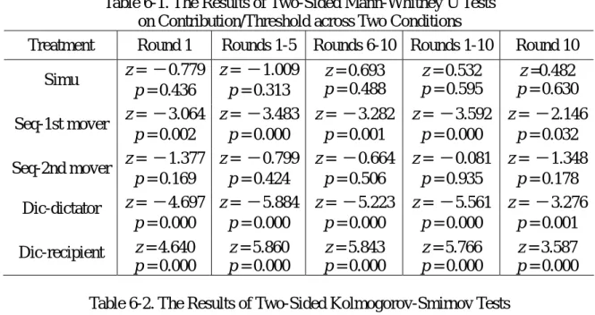
Table 6-1. The Results of Two-Sided Mann-Whitney U Tests on Contribution/Threshold across Two Conditions

Treatment Round 1 Rounds 1-5 Rounds 6-10 Rounds 1-10 Round 10 Simu z = －0.779 p = 0.436 z = －1.009 p = 0.313 z = 0.693 p = 0.488 z = 0.532 p = 0.595 z =0.482 p = 0.630 Seq-1st mover z = －3.064 p = 0.002 z = －3.483 p = 0.000 z = －3.282 p = 0.001 z = －3.592 p = 0.000 z = －2.146 p = 0.032 Seq-2nd mover z = －1.377 p = 0.169 z = －0.799 p = 0.424 z = －0.664 p = 0.506 z = －0.081 p = 0.935 z = －1.348 p = 0.178 Dic-dictator z = －4.697 p = 0.000 z = －5.884 p = 0.000 z = －5.223 p = 0.000 z = －5.561 p = 0.000 z = －3.276 p = 0.001 Dic-recipient z = 4.640 p = 0.000 z = 5.860 p = 0.000 z = 5.843 p = 0.000 z = 5.766 p = 0.000 z = 3.587 p = 0.000

Table 6-2. The Results of Two-Sided Kolmogorov-Smirnov Tests on Contribution/Threshold across Two Conditions

Treatment Round 1 Rounds 1-5 Rounds 6-10 Rounds 1-10 Round 10 Simu z = 0.559 p = 0.913 z = 0.671 p = 0.759 z = 0.224 p = 1.000 z = 0.335 p = 1.000 z = 0.224 p = 1.000 Seq-1st mover z = 1.739 p = 0.005 z = 1.897 p = 0.001 z = 1.897 p = 0.001 z = 2.055 p = 0.000 z = 1.739 p = 0.005 Seq-2nd mover z = 1.423 p = 0.035 z = 0.791 p = 0.560 z = 0.791 p = 0.560 z = 0.474 p = 0.978 z = 1.423 p = 0.035 Dic-dictator z = 2.916 p = 0.000 z = 3.607 p = 0.000 z = 3.491 p = 0.000 z = 3.491 p = 0.000 z = 2.794 p = 0.000 Dic-recipient z = 3.137 p = 0.000 z = 3.717 p = 0.000 z = 3.717 p = 0.000 z = 3.601 p = 0.000 z = 3.020 p = 0.000

Figure 1. Contribution/Threshold in the Condition T=w 0 0.1 0.2 0.3 0.4 0.5 0.6 0.7 0.8 0.9 1 1 2 3 4 5 6 7 8 9 10 Round Co nt ri b u ti on/ T

Simu Seq-1st player Seq-2nd player Dic-dictator Dic-recipient

Figure 2. Contribution/Threshold in the Condition T>w

0 0.1 0.2 0.3 0.4 0.5 0.6 0.7 0.8 0.9 1 1 2 3 4 5 6 7 8 9 10 Round Co nt ri b u ti on/ T

REFERENCES

Andreoni, J. (1988), “Why Free Ride: Strategies and Learning in Public Goods Experiments,”

Journal of Public Economics, 37, 291-304.

Andreoni, James, Paul M. Brown, and Lise Vesterlund (2002), “What makes an allocation fair? Some experimental evidence,” Games and Economic Behavior 40, 1-24.

Bolton, Gary E. and Rami Zwick (1995), “Anonymity versus Punishment in Ultimatum Bargaining,” Games and Economic Behavior, 10, 95-121.

Camerer, C.F. and R.H. Thaler (1995), “Ultimatums, Dictators and Manners,” Journal of

Economic Perspectives, 9, 209-219.

Davis, D.D. and C.A. Holt (1993), Experimental Economics, Princeton University Press, Princeton, New Jersey, U.S.A.

Forsythe, R., J.L. Horowitz, N.E. Savin, and M. Sefton (1994), “Fairness in Simple Bargaining Experiments,” Games and Economic Behavior, 6, 347-69.

Güth, Werner, R. Schmittberger, and B. Schwarze (1982), “An Experimental Analysis of Ultimatum Bargaining,” Journal of Economic Behavior & Organization, 3, 367-388. Güth, W. and R. Tietz (1990), “Ultimatum Bargaining Behavior: A Survey and

Comparison of Experimental Results,” Journal of Economic Psychology, 11, 417-49. Marwell, G. and R.E. Ames (1981), “Economists Free Ride, Does Anyone Else?” Journal of

Public Economics, 15, 295-310.

Ochs, J. and A.E. Roth (1989), “An Experimental Study of Sequential Bargaining,”

American Economic Review, 79, 355-384.

Prasnikar, Vesna and Alvin E. Roth (1992), “Considerations of Fairness and Strategy: Experimental Data from Sequential Games,” Quarterly Journal of Economics, 107(3), 865-888.

Roth, A.E., V. Prasnikar, M. Okuno-Fujiwara, and S. Zamir (1991), “Bargaining and Market Behavior in Jerusalem, Liubljana, Pittsburgh, and Tokyo: An Experimental Study,” American Economic Review, 81, 1068-1095.