產業需求與公司技術水準對公司債評價及資本結構之影響

行政院國家科學委員會專題研究計畫 成果報告

產業需求與公司技術水準對公司債評價及資本結構之影響

計畫類別： 個別型計畫 計畫編號： NSC94-2416-H-004-046- 執行期間： 94 年 08 月 01 日至 95 年 07 月 31 日 執行單位： 國立政治大學金融系 計畫主持人： 廖四郎 計畫參與人員： 黃星華；江淑玲 報告類型： 精簡報告 處理方式： 本計畫可公開查詢

中 華 民 國 95 年 7 月 10 日

產業需求與公司技術水準對公司債評價及

資本結構之影響

摘要

本研究提出並檢驗一個部分均衡模型來探討總體、產業與個體因素對公司負債比 率之影響。本研究將原有的公司資本結構或有求償權模型，擴展為一個既能考慮 總體產業需求亦可反應個體公司供給的新模型。本模型之理論預測與台灣 130 家製造業上市公司從 1994 年第 4 季到 2003 年第 4 季之實證結果相符。結果顯示 最適負債比率與資金成本和平均產業工資成正向關係，與總體需求和公司生產力 平均成長率、需求彈性和勞動與資本產出彈性成反向關係。此外，由 SUR 的估 計結果，我們發現不同的產業可能存在完全不同的特性。 關鍵字: 產業需求、公司技術水準、最適資本結構

The Impacts of Industry Demand Shocks and

Firm-Level Technology Shocks on the Valuation of

Corporate Debts and Capital Structure

Abstract

This research develops and examines a partial equilibrium model to investigate the effects of the macroeconomic, industry, and microeconomic factors on the firm-level debt ratio. The model extends the contingent-claims models of the firm’s capital structure to take into consideration not only the macroeconomic demand conditions, but also the microeconomic firm-level supply conditions. Our model predictions are generally supported by the pooled feasible generalized least squares estimations of the 130 Taiwanese manufacturing firms in the period from 1994:Q4 to 2003:Q4, where the optimal debt ratio is positively correlated to the cost of capital and the mean industry wage but is negatively correlated to the mean growth rates of the macroeconomic demand and the firm-level productivity, the elasticity of demand, and the output elasticities of labor and capital. In addition, the seemingly unrelated regression estimation for each industry further shows different industries may lead to quite diverse properties.

I. Introduction

Since the celebrated work of Modigliani and Miller (1958, 1963), the optimal capital structure has becoming one of the most important fields in corporate finance. Traditionally, both theoretical and empirical studies focus on the effect of firm-specific variables (e.g., size, profitability, tax shields…etc.) on firm’s target leverage. However, little attentions have been paid to the effects of industry demand and firm level productivity on the optimal capital structure. This is rather surprising because the state of the economy in the business cycle and the firm-level productivity both have significant impacts on the firm’s bankruptcy risk and the valuation of corporate debts, and in turn on the firm’s optimal capital structure. The present research makes an attempt to construct a partial equilibrium model with consideration of both the industry demand and firm-level productivity and further conducts the test to investigate the model implications by using the quarterly data of the 311 manufacturing firms in Taiwan form 1994 to 2003.

Traditionally, most financial economists pay a great attention to qualitative analysis of the firm’s capital structure, while some recent paper attempts to provide quantitative guidance for the optimal capital structure. Pioneered by Merton (1974), Black and Cox (1976), and Brennan and Schwartz (1978), who employ the option pricing technique to value corporate securities,1 the literature on the quantitative analysis of the optimal capital structure has been substantially developed. For example, Leland (1994) and Leland and Toft (1996) construct an optimal capital structure model with consideration of the shareholder’s endogenous bankruptcy decision, and Goldstein et al. (2001) further provide an EBIT-based optimal capital structure model.

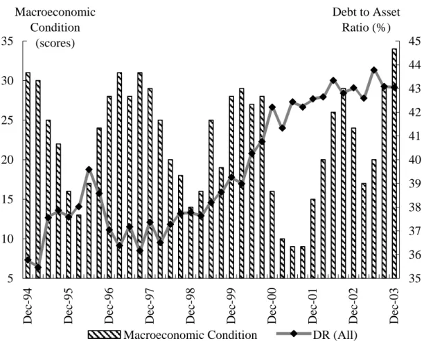
During the period of recession, the consumption demand is likely to be cut back, and hence the debtholders of the firm will suffer from increasing default risk. Duffie and Singleton (2003) report that macroeconomic conditions may affect the probability of default. They find that the correlation between the four-quarter moving averages of default rates for the speculative-grade bonds and the GDP growth rates in the sample period 1983-1997 is about -0.78, showing the negative correlation is evident, especially in the recession period 1990-1991. Moreover, Korajczyk and Levy (2003) analyze the debt to asset ratios for the aggregate data of American non-financial firms and find the systematic peaks appear during economic downturns over the last fifty years. As for our data of Taiwanese manufacturing firms, the negative relationship between the debt ratios and macroeconomic conditions also prevails. Figure 1 shows the relationship between the macroeconomic conditions (such as the total score of current business monitoring indicators)2 and the average debt ratios of the 130 Taiwanese manufacturing firms in the sample period 1994:Q4-2003:Q4. During the boom periods of 1994:Q4, 1995:Q1, 1997:Q1, and 1997:Q3, the average debt ratios are relatively low and the correlation of the 130 manufacturing firms is about -0.29. Specifically, the correlation of Plastic, Petrochemical, Chemical, and Rubber (PPCR) industry is about -0.37, while the correlation of Electronic and Information Technology (EIT) industry is about 0.095. In addition, Korajczyk and Levy (2003) provide evidence of how the macroeconomic conditions and firm-specific factors affect capital structure choices. Taking the target capital structure of the firm as a

1

This approach is the so-called real options approach or contingent claims analysis, which is also used to price credit risk and known as the firm value model or the structural model.

2

The score is monthly issued by Council for Economic Planning and Development, Executive Yuan, Taiwan.

5 10 15 20 25 30 35

Dec-94 Dec-95 Dec-96 Dec-97 Dec-98 Dec-99 Dec-00 Dec-01 Dec-02 Dec-03

Macroeconomic Condition (scores) 35 36 37 38 39 40 41 42 43 44 45 Debt to Asset Ratio (%)

Macroeconomic Condition DR (All)

Figure 1 The Relationship between Macroeconomic Condition and Debt to Asset Ratio. The macroeconomic condition is measured by the total score of current business monitoring indicators, and the sample mean debt to asset ratio, DR (All), is defined as the average of the firm’s total debt book value divided by the total asset book value.

function of the macroeconomic conditions and firm-specific variables, they find that the target leverage is pro-cyclical for the financially constrained firms, but counter-cyclical for the unconstrained ones. The firm’s optimal capital structure is indeed dependent on macroeconomic conditions; however, the existing qualitative optimal capital structure models are constructed without consideration of the macroeconomic demand conditions.

As for the microeconomic firm-specific supply conditions, most quantitative capital structure models take the total asset value or unlevered asset value as the underlying asset to price the firm’s liability, and then derive the firm’s optimal capital structure (such as Leland (1994) and Leland and Toft (1996)). Goldstein et al. (2001) provide a pioneering view that the unlevered asset value results from the expected present value of the cumulative earnings before interest and taxes (EBIT). Nevertheless, they do not explicitly demonstrate how fundamental firm-level production variables, such as the returns to scale and firm-level technology, affect the unlevered asset value. The firm-level microeconomic conditions definitely have significant impacts on EBIT and the unlevered asset value, and therefore on the liability value and optimal capital structure, especially for the manufacturing industry. However, as far as we know, none of the existing theoretical literature takes these

factors into consideration.

The macroeconomic industry demand conditions and microeconomic firm-level supply factors have notable impacts not only on the default risk of the debt issuer, but also on the valuation of corporate debts, as well as on the leverage ratio or the optimal capital structure of the firm. When the firm determines the optimal leverage by incorporating the tradeoff between tax benefits and bankruptcy costs, both the benefits and costs should depend on industry demand shocks and firm-level technology shocks. This is because the tax benefits and bankruptcy costs are associated with the cash flows of the firm, and the level of the cash flows, in turn, is relevant to whether the economy (demand) is in an expansion or contraction and whether the firm-level production (technology) is magnified or minified. Accordingly, the changes of the macroeconomic demand conditions and microeconomic supply factors, undoubtedly, should lead to variations in the firm’s optimal capital structure. The present research attempts to construct a partial equilibrium firm value model in which the cash flows incorporate both the macroeconomic demand shocks and firm-level supply shocks, and further analyzes the properties of the firm’s optimal capital structure. The effects of the elasticity of demand and the output elasticities of labor and capital on the optimal capital structure are particularly taken into consideration. According to the empirical analysis, the model implications are generally supported by the data of the 130 Taiwanese manufacturing firms in the period from 1994:Q4 to 2003:Q4. The distinctions among six manufacturing industries (including Food; Plastic, Petrochemical, Chemical and Rubber; Textile; Machine-Driven; Iron and Steel; Electronic and Information Technology) are further investigated. Our model definitely provides additional insights as well as complements to both the earlier theoretical and empirical studies about the firm’s optimal capital structure.

The rest of this research is organized as follows. Section 2 provides the theoretical model, and the implications are given in Section3. In Section 4, we empirically test the implications, and investigate differences among the six manufacturing industries. Section 5 summarizes and makes concluding remarks.

II. The Model

Consider an industry consisting of a representative firm, and suppose the information is perfect and complete. In addition, all agents are risk-neutral, and thus discount cash flows at a constant risk-free rate r >0. This risk-neutrality assumption is innocuous. If agents are not risk-neutral, the analysis may be conducted under the risk-neutral probability measure (see Harrison and Kreps (1979)) where the risk premium is incorporated. Time domain is continuously varying over [0, )∞ , and moreover, uncertainty is represented by a filtered probability space

(

Ω, ,F Q

)

over which all stochastic processes are defined with respect to their corresponding regular filtrations.

1. Macroeconomic Demand and Microeconomic Firm-Level

Productivity Shocks

The Firm’s demand, governed by the law of demand, is a decreasing function of output price. The inverse demand function of the firm is given by

1

( ) ( ) _d ,

P t =h t Y− ε (1) where P is the output price, Y_d is the demand of the industry, ε >0 is the

elasticity of industry demand, and h represents the macroeconomic demand shocks, reflecting the state of the economy, which is governed by a geometric Brownian motion as follows:

( ) ( ), (0) 0 given, ( ) h h h dh t dt dW t h h h t =μ +σ ≡ > (2)

where μ_h and σ_h are two positive constants denoting the drift and diffusion terms of the industry demand shocks, and W_h is a Wiener process defined on

(

Ω, ,F Q

)

.

The firm’s production function or output Y_s is assumed to be a standard Cobb-Douglas form, which is the mostly used type as given by

( ) ( ) a b,

s t t

Y t = A t L K (3) where L is labor demand; K is capital demand; a b, ∈(0,1) respectively show the

output elasticities of labor and capital and their sum represents the returns to scale (take a b+ =1 for example, it implies constant returns to scale); A is the firm-level productivity (microeconomic supply) shocks governed by a geometric Brownian motion as below. ( ) ( ), (0) 0 given, ( ) A A A dA t dt dW t A A A t =μ +σ ≡ > (4)

where μA and σA are two positive constants denoting the drift and diffusion terms,

and W is a Wiener process defined on _A

(

Ω, ,F Q

)

. The instantaneous correlation coefficient between the macroeconomic demand shocks and the microeconomic firm-level productivity shocks is denoted as ρ_hAdt=EQ

[

dW dW_{h A}

]

.

2. The Dynamics of the Firm’s Unlevered Asset Value

Assume the input markets are competitive, and thus the firm takes the wage of labor

w and the cost of capital r as given. The profit function of the firm is given by the _k

value function of the following maximization problem:

, 1 max ( ) ( ) . . ( ) ( ) ; ( ) ( ) . t t s t k t L K a b d s t t P t Y t wL r K s t P t h t Y− ε Y t A t L K − − = = (5)

After applying the following market-cleaning condition Y_d =Y_s , at each instantaneous time, we can set the profit function as a function of the levels of h and

A . Solving this problem yields the profit function

(

h A a b w r_t, _t; , , , ,_k

) ( ) ( )

h_t y A_t z,

π ε =η (6)

where η= −

(

1 w

(

1−b a x

)

₁

)

( ) (x₁ θy x₂)b z , θ =(a b+ )(ε−1) ε , x₁=aθ

[

w a b( + )

]

,

2 ( ) ( k )

x = wb r a , y=1 (1−θ), and z=θ

[

(1−θ)(a b+ )

]

. Here the profit function can be explained as the earnings before interest and taxes (EBIT) of the firm at each date t , which is the origin of the unlevered asset value. As a consequence, we define

(

)

( )t h A a b w r_t, _t; , , , ,_k

δ =π ε as the EBIT of the firm hereafter. Applying the product rule of Itô’s lemma with simplification, the dynamic process of the EBIT can be shown to be ( ) ( ), ( ) d t dt dW t t δ δ δ δ _{μ σ} δ = + (7) where μ_δ = yμ_h +zμ_A+0.5 (y y−1)σ_h2+0.5 (z z−1)σ_A2+yzσ σ ρ_{h A hA},

(

2 2

)

(y h) 2yz h A hA (z A) δ σ = σ + σ σ ρ + σ , and

Following Goldstein et al. (2001), the unlevered asset value of the firm V is the value of the claim to the entire EBIT, which can be defined as

( ) E ( ) rs _t , t V t = ⎡_⎢ ∞δ s e− ds ⎤_⎥ ⎣

∫

⎦ Q _F (8)

where F_t is the information set (sigma field) generated by W_δ up to time t . According to Equation (7), the unlevered asset value at time t can be calculated as

( ) (t r _δ)

δ −μ where we assume r−μ_δ > . Accordingly, we can further show that 0 ( ) ( ) ( ). ( ) dV t t dt rdt dW t V t δ δ δ _σ + = + (9)

3. The Firm’s Optimal Capital Structure

We take the firm’s debt as a function of the firm’s unlevered asset value. Because coupon payments of the debts are tax deductible, the firm has an incentive to issue debts. Debt contracts in our model are assumed to be perpetual, issued at par value P with flow of coupon payments C to the debtholders, while the remaining EBIT accrues to the shareholders. If the firm declares default on its debts, the debtholders immediately obtain the liquidation value (1−α)V_B, and the shareholders get nothing, where (0,1)α∈ is the ratio of bankruptcy costs, and V_B

(

< ≡V δ(0) (r−μ_δ)

)

is the bankruptcy trigger which is now an exogenous constant but will be endogenously determined later. By the risk-neutral pricing method, the value of the corporate debt can be written as

(

;

)

E ₀B rs E (1 ) rB , B B D V V = _⎢⎡ τ Ce− ds⎤_⎥+ ⎡_⎣ −α V e−τ ⎤_⎦ ⎣

∫

⎦ Q Q (10)

where τ_B =inf

(

t>0; ( )V t ≤V_B

)

denotes the first passage time that the unlevered asset value goes down and touches the bankruptcy trigger V . It can be shown that _B

the debt value is equal to

(

; _B

)

1 (1 ) _B , B B C V V D V V V r V V γ γ α − − ⎛ _{⎛ ⎞} ⎞ _{⎛ ⎞} ⎜ ⎟ = −_{⎜ ⎟} + − _{⎜ ⎟} ⎜ _{⎝ ⎠} ⎟ _{⎝ ⎠} ⎝ ⎠ (11) where γ =⎜⎛μδ −0.5σδ2+

(

μδ −0.5σδ2

)

2+2rσδ2⎟⎞ σδ2 ⎝ ⎠ , and

(

V VB

)

γ − can be

explained as the risk-neutral state price of the firm’s bankruptcy filing. The derivation is provided in the Appendix.

Following Leland (1994), the total firm value is equal to the unlevered asset value plus the tax benefits minus the bankruptcy costs. Therefore, the value of the total firm value can be shown as

(

)

0 ; E E 1 , B B r rs B B B B B F V V V Ce ds V e C V V V V r V V τ _τ γ γ τ α τ _α − − − − ⎡ ⎤ _{⎡ ⎤} = + _{⎢ ⎥}− _{⎣ ⎦} ⎣ ⎦ ⎛ _{⎛ ⎞} ⎞ _{⎛ ⎞} ⎜ ⎟ = + −_{⎜ ⎟} − _{⎜ ⎟} ⎜ _{⎝ ⎠} ⎟ _{⎝ ⎠} ⎝ ⎠

∫

Q Q (12)

where τ is the effective corporate tax rate. The derivation is also provided in the Appendix.

According to the accounting identity of the balance sheet that the total firm value must equal the sum of the equity and liability values, the equity value can therefore be expressed as

(

)

(

)

(

)

(1 ) (1 ) ; _B ; _B ; _{B B} . B C C V E V V F V V D V V V V r r V γ τ τ ⎛ ⎞− − ⎛ − ⎞ = − = − +_⎜ − _{⎟⎜ ⎟} ⎝ _{⎠⎝ ⎠} (13)

Next, the endogenous optimal bankruptcy strategy is going to be determined. As far as the shareholders are concerned, the firm can decide when to declare bankruptcy by optimally choosing the default trigger taking account of not only the macroeconomic demand shocks but also the microeconomic firm-level productivity shocks. The solution of the following smooth-pasting condition shows that the firm optimally determines the bankruptcy trigger to maximize the equity value:3

(

)

(

)

* * ; ; 0. B B B B B V V V B B V V V E V V E V V V V = = = = ∂ ∂ = = ∂ ∂ (14)

Solving Equation (14) yields

* (1 ) . 1 B C V r τ γ γ − = + (15)

After substituting the optimal bankruptcy trigger into Equations (11)-(13), we complete the derivation of the firm’s optimal capital structure, and define the firm’s optimal debt ratio as DR V V( ; _B*)= D V V( ; _B*) F V V( ; _B*).

III. Theoretical Implications

This section attempts to investigate the theoretical implications concentrating on the effects of the mean growth rates of the industry demand and the firm level productivity on the firm’s optimal debt ratio. To clearly identify the comparative static results of the model, we first set some reasonable parameters. Let the coupon payments C=800,4 the corporate effective tax rate τ =0.35, and the proportional bankruptcy costs α =0.5. The coupon payment is set to approximate the bond yields of 8%, i.e., P=10000, while the tax rate and proportional bankruptcy costs are set to be the same as those of Leland (1994). The risk-free interest rate as well as all the other parameters are adopted from the averages in the sample period, given as follows:

0.055

r= , h=22.5 , A=1.2, 0.03μ_h = , 0.004μ_A = , 0.26σ_h = , 0.18σ_A = , 0.0001

hA

ρ = − , a=0.37, b=0.65, ε =1.3, 0.068r_k = , w=3.4.5

Result 1. The optimal debt ratio DR is positively correlated to the cost of capital *

k

r and the mean wage w, but is negatively correlated to the mean growth rate of the macroeconomic demand μ_h and the elasticity of demand ε .

The intuition of Result 1 is as follows. Other things being equal, when the prices of inputs, r and _k w, rise, the production costs would increase as well. The firm’s revenue (EBIT) (in turn the unlevered asset value) must decrease; therefore, the liability value and total firm value would both go down, while the debt ratio will increase. This is because the liability value is concave but the total firm value is convex to the unlevered asset value. Moreover, it is also consistent with the pecking order theory, i.e., equity is the last financing choice. When the prices of inputs rise, the firm raises its liability (in turn raises the debt ratio), to cover these costs if they do not prefer using equity financing.

3

See Leland (1994). 4

All the dollar amounts in the research are expressed in ten thousands of New Taiwan dollars. 5

The optimal debt ratio is negatively correlated to the mean growth rate of macroeconomic demand, namely, it is counter-cyclical. This is because when the demand is magnified, other things being equal, the firm’s revenues (EBIT) would increase, implying that the firm’s unlevered asset value goes up as well. Therefore, the liability value must increase due to the decreasing possibility of the firm’s bankruptcy filing, which is bounded by the risk-less value C r. On the other hand, when the unlevered asset value goes up, the total firm value would also increase without any upper bound. Accordingly, the increase of the total firm value will dominate that of the liability value, and hence, the higher the firm’s revenue is, the lower the debt ratio would be. As for the elasticity of industry demand ε , when the elasticity rises, other things being equal, the output price would also increase (in turn the firm’s revenue (EBIT) rises), and therefore the debt ratio would decrease.

Result 2. The optimal debt ratio DR is negatively correlated to the output * elasticities of labor and capital, a and b , and the mean growth rate of the firm-level productivity μ_A.

The above result is as expected. Not only higher output elasticities of production inputs but also greater firm-level productivity would result in greater production of the firm. As a result, other things being equal, the firm’s revenue must again rise, and the optimal debt ratio would subsequently decrease.

IV. Empirical Evidence

1. Data and Variables

We select 130 Taiwanese manufacturing firms across six industries, including Food, Plastic, Petrochemical, Chemical, and Rubber (PPCR), Textile, Machine-Driven (MD), Iron and Steel (IS) and Electronic and Information Technology (EIT) industry from the period 1994:Q3 to 2003:Q4. All needed data series are collected from Taiwan Economic Journal Data Bank (TEJ DB).

As for the macroeconomic variables, the total score of current business monitoring indicators is the proxy of the macroeconomic demand shocks h, and the mean growth rate μ_h can be thus obtained. The elasticity of demand is calculated by6 ( ) ( 1) ( 1) ( ) ( 1) ( 1) d d d t d d Y P Y t Y t P t P Y P t P t Y t ε = −Δ = − − − − Δ − − − ,

where P is measured as the price index of Taiwanese manufacturing industry, and

d

Y is calculated from the total sales of Taiwanese manufacturing industry PY . As _d

mentioned by Levinsohn and Melitz (2003), output is typically measured not in physical units but rather in terms of dollars, i.e., sales. In reality, one usually observes the value of sales at the industry. Because sales depends on the price which is, in turn, determined in the market equilibrium, and the estimation of industry demand, typically thought of as a demand-side phenomenon, depends crucially on the supply side of the market. In addition, the price of labor w is estimated by the mean wage of Taiwanese manufacturing industry, and the price of capital r is measured by the _k

loan rate of capital expenditures in Taiwan.

The firm-level data are employed to estimate the microeconomic variables. First, the elasticities of labor and capital, a and b, are respectively calculated by

6

( ) ( 1) ( 1) ( ) ( 1) ( 1) s s s t s s Y L Y t Y t L t a L Y L t L t Y t Δ − − − = = Δ − − − , and ( ) ( 1) ( 1) ( ) ( 1) ( 1) s s s t s s Y K Y t Y t K t b K Y K t K t Y t Δ − − − = = Δ − − − .

Similar to the estimation of Y , the estimation of _d Y is extracted from the data of _s

firm-level net sales PY , where P again is the price index of Taiwanese _s

manufacturing firms. If the firm produces homogeneous goods, the firm-level sales deflated by the price index for the industry yield a perfect proxy for the unobserved physical output. Moreover, L and K are estimated by the firm-level operating expenses and operating costs which are respectively regarded as wL and r K . As _k

before, w is the mean wage of Taiwanese manufacturing industry and r is the loan _k

rate of capital expenditures. According to Business Entity Accounting Law of Taiwan, the firm-level operating expenses are mainly contributed by the firm-level wage expenses, taken as the proxy for wL, while the firm-level operating costs consisting of other capital costs are served as the proxy for r K . Finally, the firm-level _k

productivity A is specifically measured by the exponent of the firm-level gross profit margin which is the firm-level realized gross profit divided by the firm-level net sales. Taking exponent is to maintain the non-negativity property which is consistent with the log-normal assumption of the firm-level productivity.

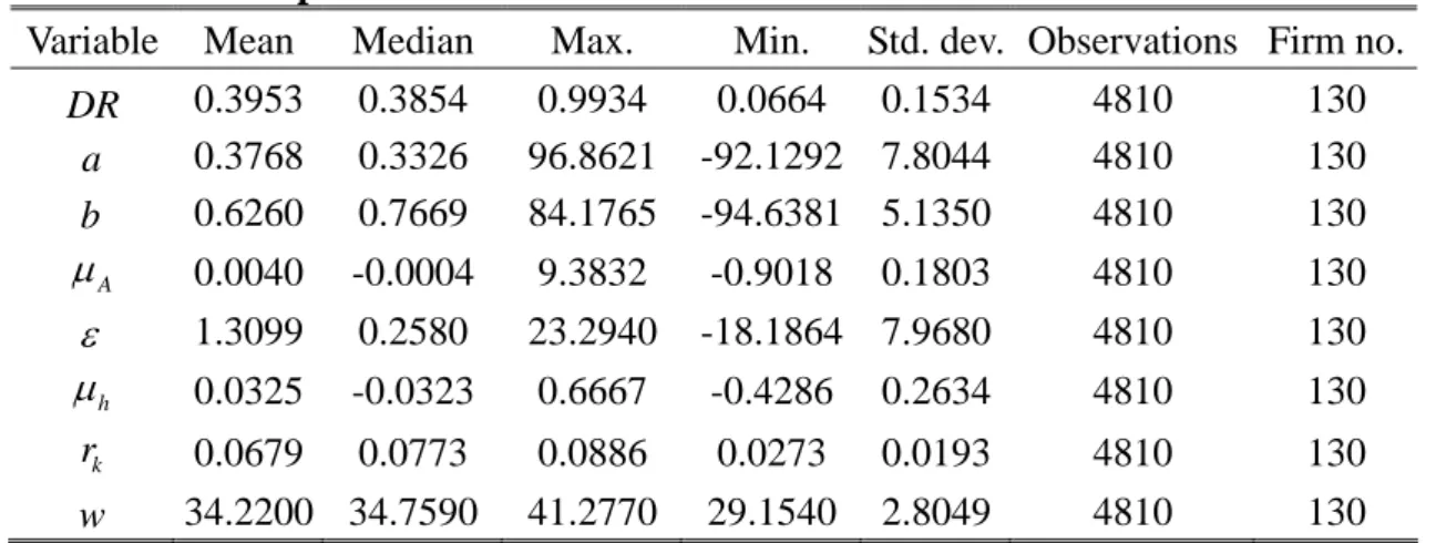
The dependent variable, the firm-level debt ratio DR is calculated as the total debt book value divided by the total asset book value. The sample consists of the 130 Taiwanese manufacturing firms across 37 periods (quarters) from 1994:Q4 to 2003:Q4. The descriptive statistics of the above variables are summarized in Table 1.

Table 1 Descriptive Statistics of Variables

Variable Mean Median Max. Min. Std. dev. Observations Firm no.

DR 0.3953 0.3854 0.9934 0.0664 0.1534 4810 130 a 0.3768 0.3326 96.8621 -92.1292 7.8044 4810 130 b 0.6260 0.7669 84.1765 -94.6381 5.1350 4810 130 A μ 0.0040 -0.0004 9.3832 -0.9018 0.1803 4810 130 ε 1.3099 0.2580 23.2940 -18.1864 7.9680 4810 130 h μ 0.0325 -0.0323 0.6667 -0.4286 0.2634 4810 130 k r 0.0679 0.0773 0.0886 0.0273 0.0193 4810 130 w 34.2200 34.7590 41.2770 29.1540 2.8049 4810 130

Notes: The variables are defined as follows. DR is the firm-level debt ratio; a and

b are the firm-level output elasticities of labor and capital, respectively; μ_A is the mean growth rate of the exponential firm-level gross profit margin; ε is the elasticity of industry demand; μ_h is the mean growth rate of the total score of current business monitoring indicators; r is the loan rate of capital expenditures and _k

w is the mean wage of Taiwanese manufacturing industry expressed in thousand dollars.

2. Pooled Generalized Least Squares (PGLS) Regression

model predictions. Because the firm-level debt ratio is significantly one-period auto- correlated, the following regression is conducted:

,

, 0 1 , 1 2 , 3 , 4 _{i t} 5 6 _t 7 _t 8 ,

i t i t i t i t A t h k t i t

DR = +c c DR ₋ +c a +c b +c μ +cε +c μ +c r +c w +e (16) where 1, 2,...,130i= and t=1(1994 : Q4), 2,..., 37(2003 : Q4). DR is the firm-level debt ratio; a and b are the firm-level output elasticities of labor and capital, respectively; μ_A is the mean growth rate of the exponential firm-level gross profit margin; ε is the elasticity of manufacturing industry demand; μ_h is the mean growth rate of the total score of current business monitoring indicators; r is the loan _k

rate of capital expenditures and w is the mean wage of the manufacturing industry evaluated expressed in thousand dollars. Here the macroeconomic conditions, ε , μ_h,

k

r and w, do not vary across firms but across time periods.

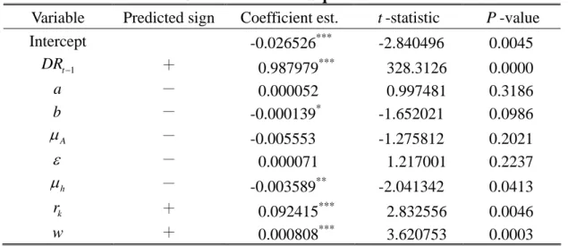
Estimation of Equation (16) is achieved using the pooled cross-section time series data. Table 2 shows the feasible generalized least squares estimations of the pooled cross-section time-series regression, accounting for cross-equation heteroskedasticity by minimizing the weighted sum of squared residuals. The weights are the inverse of the estimated equation variances derived from the unweighted estimation of the parameters of the system. Therefore, pooled cross-section time-series regression allows firm-level debt ratios to vary across both companies and times, resulting in more efficient parameter estimates due to the greater variation of the data. The regression results generally support the model implications, especially those of the macroeconomic conditions. Observe that the positive effects of the loan rate of capital expenditures and the mean wage of the manufacturing industry as well as the negative effect of the mean growth rate of the total score of current business monitoring indicators are quite significant as predicted by our model, but they have been ignored in the previous theoretical literature. As for the microeconomic variables, the effects of the firm-level output elasticity of capital and the mean growth rate of the exponential firm-level gross profit margin are consistent with the model implications, where the former is statistically significant but the latter is not. The two inconsistent variables, the output elasticity of labor a and the elasticity of industry demand ε , are rather dispersed across industries, and therefore would not agree with the model predictions. Overall speaking, the regression has an adjusted R-squared of 0.9801, with the Durbin-Watson statistic of 2.1034.

Table 2 Pooled Feasible Generalized Least Squares Estimation Results Variable Predicted sign Coefficient est. t -statistic P -value

Intercept -0.026526*** -2.840496 0.0045 1 t DR₋ ＋ _0.987979*** 328.3126 0.0000 a － _{0.000052 0.997481 0.3186} b － _-0.000139* -1.652021 0.0986 A μ － _{-0.005553 -1.275812 0.2021} ε － _{0.000071 1.217001 0.2237} h μ － _-0.003589** -2.041342 0.0413 k r ＋ _0.092415*** 2.832556 0.0046 w ＋ _0.000808*** 3.620753 0.0003

Notes: Dependent variable is the firm-level debt ratio DR , and independent variables _t

are: the one-period lagged debt ratio DR_t−1; the firm-level output elasticities of labor and capital, a and b , respectively; the mean growth rate of the exponential firm-level gross profit margin μ_A; the elasticity of manufacturing industry demand

ε ; the mean growth rate of the total score of current business monitoring indicators

h

μ ; the loan rate of capital expenditures r and the mean wage of manufacturing _k

industry expressed in thousand dollars w. The F-statistic, 28,954, is considerably high, and the adjusted R-squared of the regression is 0.9801, with the Durbin-Watson statistic of 2.1034. The notations *, ** and *** signify the 10%, 5%, 1% confidence levels, respectively.

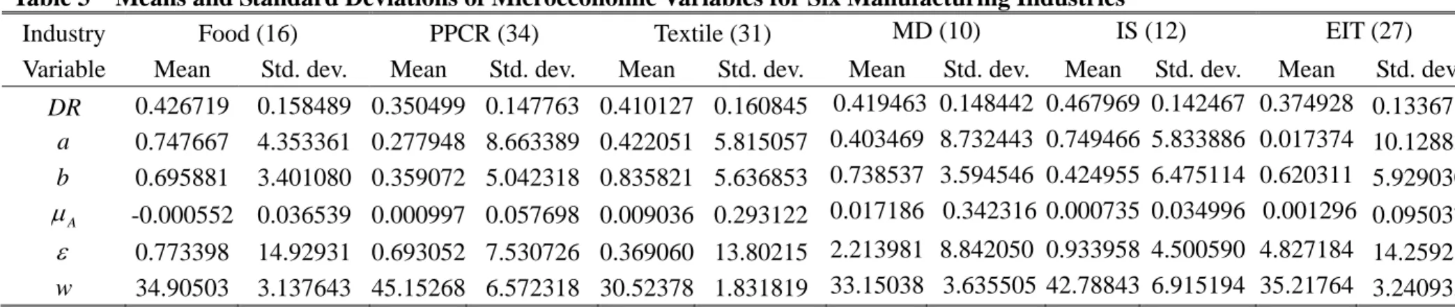
In what follows, according to the classification of Taiwan Stock Exchange Corporation (TSEC), we divide the 130 Taiwanese manufacturing firms into six industries, including Food, Plastic, Petrochemical, Chemical, and Rubber (PPCR), Textile, Machine-Driven (MD), Iron and Steel (IS) and Electronic and Information Technology (EIT) to investigate the distinctions among different industries. Table 3 summarizes the descriptive statistics of the microeconomic factors across six manufacturing industries, while the other macroeconomic conditions are the same as those of Table 1. In view of Table 3, the characteristics across industries are quite distinct. For example, Textile industry has the highest labor share of 0.84, and IS industry has the highest capital share of 0.75, while EIT industry has the greatest difference between the labor and capital share, about 0.60. The reason is that Textile industry is a light industry mainly depending on labor, and IS industry is a heavy industry essentially relying on capital, while EIT industry is a high-tech industry, demanding low labor but high capital. Moreover, the elasticity of the industry of living goods, such as that of Textile industry, 0.37, is much less than that of the industry of luxury goods, such as that of EIT industry, 4.83.

Subsequently, the individual seemingly unrelated regression is conducted for each of the six manufacturing industries to investigate the performance in individual industry and explore the differences among industries.

3. Seemingly unrelated Regression (SUR) in Different Manufacturing Industries

The above analysis has not differentiated debt ratios among different industries. However, such a distinction may be important that it may lead to different inferences with respect to the effect of some variables in the model, and may thus have varying impacts on the firm-level debt ratios due to differences within each manufacturing industry. For example, the business cycle, such as the total score of current business monitoring indicators, may have a particular impact on debt ratios of different industries. To examine differences among industries in a more systematic way, the Zellner’s seemingly unrelated regression (SUR) is conducted separately on the firm-level debt ratios for the following manufacturing industries: Food, Plastic, Petrochemical, Chemical, and Rubber (PPCR), Textile, Machine-Driven (MD), Iron and Steel (IS) and Electronic and Information Technology (EIT). The SUR system is as follows: , , 0 1 , 1 2 , 3 , 4 j 5 6 7 8 , t t i t j j j j j j j j j j j j j j j j i t i t i t i t A t h k t i t DR =c +c DR ₋ +c a +c b +c μ +c ε +c μ +c r +c w +e , (17) where j= Food, PPCR, Textile, MD, IS and EIT, and other notations are the same as those of Equation (16). The major difference between the regression (16) and the SUR system (17) is the industry price index P is now extracted from each of the six

industries. This is relevant to the calculations of Y and _s Y , which in turn affect the _d

calculations of the elasticities, a, b and ε . In addition, the industry mean wage

w is also collected separately from each industry.

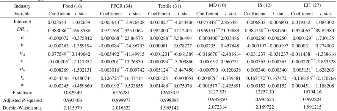
The (cross-section) SUR results, with the correction of cross-section heteroskedasticity and contemporaneous correlation in the feasible GLS specifications, are reported in Table 4. The results among industries are quite different. First, the estimations of PPCR industry are all very significant, and are consistent with those of the pooled FGLS, showing the firms on the PPCR industry behave much like the average one of the whole manufacturing industry. For the firm-level variables, the coefficients of labor share are positive for all industries except for the Food industry, and are significant for the PPCR, Textile, MD and EIT industries, while the positive effects of capital share are only significant for the PPCR and IS industry. The effect of the mean growth rate of the exponential firm-level gross profit margin is significantly negative for the PPCR, Textile and MD industries but significantly positive for the Food industry. As for the industry-specific variables, the effect of elasticity of industry demand is significantly negative for the Food, Textile and EIT industries, whereas is significantly positive for the PPCR industry. The coefficients of the industry average wage are significantly positive for the PPCR and Textile industries but significantly negative for the MD industry. As for the macroeconomic variables, the coefficients of the mean growth rate of the total score of current business monitoring indicators are significantly negative for the PPCR and Textile industries but are significantly positive for the EIT industry. The significant positive effect of the loan rate of capital expenditures reveals in the PPCR and IS industries, while the significant negative coefficients appear in the MD and EIT industries.

V. Summary and Concluding Remarks

This research develops and examines a partial equilibrium model to explore the effects of the macroeconomic, industry and microeconomic firm-level production factors on the firm-level debt ratio. The present model extends the contingent-claims models of the firm’s capital structure, such as Leland (1994) and Goldstein et al. (2001), to take into account not only the macroeconomic demand conditions, including the macroeconomic demand shocks, the elasticity of industry demand, the mean industry wage and the cost of capital, but also the microeconomic firm-level supply conditions, including the firm-level productivity shocks and the output elasticities of production inputs, labor and capital.

Our model predictions are generally supported by the pooled feasible generalized least squares estimation results of the 130 Taiwanese manufacturing firms in the sample period from 1994:Q4 to 2003:Q4. The optimal debt ratio is positively correlated to the cost of capital and the industry mean wage but is negatively correlated to the mean growth rate of the macroeconomic demand and the elasticity of demand. In addition, the optimal debt ratio is negatively correlated to the output elasticities of labor and capital and the mean growth rate of firm-level productivity. Moreover, we also conduct the seemingly unrelated regression separately for each industry, showing different industries may lead to quite diverse results and can be further used to capture the properties of the six manufacturing industries.

The findings provide us a better understanding of how both the macro and micro economic conditions affect and account for the determination of the firm’s optimal capital structure, and are of importance to investors, financial managers of firms and officials of the relevant supervisory authorities.

Table 3 Means and Standard Deviations of Microeconomic Variables for Six Manufacturing Industries

Industry Food (16) PPCR (34) Textile (31) MD (10) IS (12) EIT (27) Variable Mean Std. dev. Mean Std. dev. Mean Std. dev. Mean Std. dev. Mean Std. dev. Mean Std. dev.

DR 0.426719 0.158489 0.350499 0.147763 0.410127 0.160845 0.419463 0.148442 0.467969 0.142467 0.374928 0.133678 a 0.747667 4.353361 0.277948 8.663389 0.422051 5.815057 0.403469 8.732443 0.749466 5.833886 0.017374 10.12883 b 0.695881 3.401080 0.359072 5.042318 0.835821 5.636853 0.738537 3.594546 0.424955 6.475114 0.620311 5.929030 A μ -0.000552 0.036539 0.000997 0.057698 0.009036 0.293122 0.017186 0.342316 0.000735 0.034996 0.001296 0.095037 ε 0.773398 14.92931 0.693052 7.530726 0.369060 13.80215 2.213981 8.842050 0.933958 4.500590 4.827184 14.25921 w 34.90503 3.137643 45.15268 6.572318 30.52378 1.831819 33.15038 3.635505 42.78843 6.915194 35.21764 3.240933

Notes: The variables are defined as follows. DR is the firm-level debt ratio; a and b are the firm-level output elasticities of labor and capital, respectively; μ_A is the mean growth rate of the exponential firm-level gross profit margin; ε is the elasticity of industry demand and w is the industry mean wage expressed in thousand dollars. The industries are defined as follows. Food is the Food industry; PPCR is the Plastic, Petrochemical, Chemical, and Rubber industry; Textile is the Textile industry; MD is the Machine-Driven industry; IS is the Iron and Steel industry and EIT is the Electronic and Information Technology industry. The parentheses show the number of firms in each industry.

Table 4 Seemingly unrelated Regression Results in Different Manufacturing Industries

Industry Food (16) PPCR (34) Textile (31) MD (10) IS (12) EIT (27) Variable Coefficient t-stat. Coefficient t-stat. Coefficient t-stat. Coefficient t-stat. Coefficient t-stat. Coefficient t-stat. Intercept _{0.023544 1.032639 -0.005643}*** -3.976408 -0.033827***-4.044406 0.077848***2.856481 -0.006803 -0.006803 0.019352 1.084302 1 t DR_{− 0.983086}*** 166.8586 0.972768***925.0064 0.982000***312.2405 0.969151***71.33889 0.984750***0.984750 0.934065*** 89.82980 a _{-0.000072 -0.375842 0.000068}*** 23.86573 0.000288***5.586494 0.000400**2.033486 0.000250 0.000250 0.000129* 1.730135 b -0.000263 -1.359194 -0.000084***-24.86793 0.000081 2.078227 0.000235 0.457648 -0.000197*-0.000197 0.000031 0.274003 A μ _0.077549*** 3.149642 -0.005492***-11.49915 -0.001231**-0.661389 -0.016670**-2.481614 -0.031237 -0.031237 -0.011438 -1.338616 ε _-0.000205** -2.117352 0.000201***13.76830 -0.000094***-3.309860 0.000192 0.960731 0.000365 0.000365 -0.000220*** -3.853528 h μ _{-0.008269 -1.502131 -0.003016}*** -7.009742 -0.005124***-3.447450 -0.000790 -0.120638 0.000340 0.000340 0.005151* 1.628203 k r _{-0.044346 -0.480744 0.126724}*** 16.47414 -0.020428 -0.904054 -0.204876* -1.739481 0.167472**0.167472 -0.138185** -2.170766 w _{-0.000245 -0.459860 0.000192}*** 9.533855 0.001486***6.075076 -0.001517**-2.425891 0.000152 0.000152 0.000451 1.188208 F-statistic 10829.49 6576281 126030.9 3127.533 12257.10 16794.16 Adjusted R-squared 0.993406 0.999977 0.998895 0.985850 0.995623 0.992824 Durbin-Watson stat. 2.115979 2.016322 1.965142 2.072314 2.169722 1.991215

Notes: Dependent variable is the firm-level debt ratio DR_t, and independent variables are: the one-period lagged debt ratio DR_t−1; the firm-level output elasticities of labor and capital a and b, respectively; the mean growth rate of the exponential firm-level gross profit margin μ_A; the elasticity of manufacturing industry demand ε ; the mean growth rate of the total score of current business monitoring indicators μ_h; the loan rate of capital expenditures r and the mean _k

wage of manufacturing industry expressed in thousand dollars w. The industries are defined as follows. Food is the Food industry; PPCR is the Plastic, Petrochemical, Chemical, and Rubber Industry; Textile is the Textile industry; MD is the Machine-Driven industry; IS is the Iron and Steel industry and EIT is the Electronic and Information Technology industry. The parentheses show the firm numbers in each industry, and the notations *, ** and *** signify the 10%, 5%, 1% confidence levels, respectively.

Appendix

To derive the formulas, we need the distribution of τ_B =inf

(

t>0 : ( )V t ≤V_B

)

, which is well known and can be easily derived by the reflection principle and Girsanov’s Theorem (see, for example, Harrison (1985)). The distribution is given as follows:

(

)

(

)

1 ln( ) 2

₍

₎

2 2 2 3 Pr ln ( ; , ) , where 0.5 . 2 B V V t t B B B d t V V f t V V e dt _t δ λ σ δ δ δ τ λ μ σ πσ ⎛ + ⎞ − ⎜_⎜ ⎟_⎟ ⎝ ⎠ ≤ ≡ = = −

Because Equation (10) can be expressed as

(

)

₀ 0 0 ; E E (1 ) 1 E (1 ) E 1 (1 ) , B B B B r rs B B r r B B B B D V V Ce ds V e C e ds V e ds r C V V V r V V τ _τ τ τ γ γ α α α − − ∞ ₋ ∞ ₋ ⎡ ⎤ _{⎡ ⎤} = _{⎢ ⎥}+ _⎣ − _⎦ ⎣ ⎦ ⎛ ⎡ ⎤⎞ ⎡ ⎤ = ⎜ − _{⎢⎣ ⎥⎦}⎟+ − _{⎢⎣ ⎥⎦} ⎝ ⎠ ⎛ _{⎛ ⎞} ⎞ _{⎛ ⎞} ⎜ ⎟ = −_{⎜ ⎟} + − _{⎜ ⎟} ⎜ _{⎝ ⎠} ⎟ _{⎝ ⎠} ⎝ ⎠

∫

∫

∫

Q Q Q Q

all what we need to do is to prove

(

)

0 E rB B e τ ds V V γ ∞ ₋ − ⎡ _{⎤ =} ⎢ ⎥ ⎣

∫

⎦ Q

with the technique of

completing squares and changing variables as follows.

(

)

( )

(

)

( ) 2 * _* 2 2 ln 1 2 2 3 0 0 0 ln 1 2 _{* 2 2} 2 3 0 ln E ( ; , ) 2 ln

, where 2 (by completing squares) 2 B B B V V t t B r rt rt B V V t t B B B V V e ds e f t V V ds e e ds t V V V e ds r V _t V V δ δ _δ λ σ τ δ λ λ _λ σ _σ δ δ πσ λ λ σ πσ ⎛ + ⎞ − ⎜ ⎟ ∞ ₋ ∞ ₋ ∞ ₋ ⎜_⎝ ⎟_⎠ ⎛ − ⎞ _{⎛ + ⎞} −⎜_⎜ ⎟_{⎟ − ⎜ ⎟} ∞ ⎜ ⎟ ⎝ ⎠ _{⎝ ⎠} − ⎡ _{⎤ = =} ⎢ ⎥ ⎣ ⎦ ⎛ ⎞ =_{⎜ ⎟} = + ⎝ ⎠ ⎛ ⎞ = ⎜ ⎟ ⎝ ⎠

∫

∫

∫

∫

Q ( )

(

)

(

(

)

)

(

)

(

(

)

)

* _* 2 2 * * 2 2 ln 1 _{* *} * 2 2 3 2 3 0 2 * * 2 3 ln ln by 2 2 ln ln by 2 B V V t B t B B B B B V V t dt V V t t e ds d t t t V V t dt V V t V V d V V t t δ δ δ δ λ λ _λ σ _σ δ δ δ λ λ λ σ σ δ δ λ λ λ σ πσ πσ λ λ σ πσ ⎛ − ⎞ _{⎛ + ⎞} ⎜ ⎟ _{⎜ ⎟} ⎜ ⎟ _∞ − _{⎜ ⎟} ⎝ ⎠ _{⎝ ⎠} ⎛ − ⎞ −⎜_⎜ ⎟_⎟ − ⎝ ⎠ ⎛ _{⎛− − ⎞ −} ⎞ ⎜ ⎜_⎜ ⎟_⎟= ⎟ ⎜ _{⎝ ⎠} ⎟ ⎝ ⎠ ⎛ _{⎛− + ⎞ +} ⎞ ⎛ ⎞ ⎛ ⎞ ⎜ ⎟ =⎜ ⎟ ⎜ ⎟ _⎜ ⎜_⎜ ⎟_⎟= _⎟ ⎝ ⎠ ⎝ ⎠ _⎝ ⎝ ⎠ _⎠ =

∫

( ₂) ( ₂)2 ₂ * 2 2 0.5 0.5 2 . r B B B V V V V V V δ δ δ δ δ δ δ μ σ μ σ σ λ λ _γ σ σ ⎛ ⎞ − + − + ⎜ ⎟ ⎛ + ⎞ _{⎜ ⎟} −⎜_⎜ ⎟_⎟ − − ⎜ ⎟ ⎝ ⎠ _{⎜ ⎟} ⎝ ⎠ ⎛ ⎞ ⎛ ⎞ ⎛ ⎞ = = ⎜ ⎟ ⎜ ⎟ ⎜ ⎟ ⎝ ⎠ ⎝ ⎠ ⎝ ⎠

By the same token, Equation (12) can be therefore derived.

References

Athanassakos, G. and P. Carayannopoulos, 2001, “An Empirical Analysis of the Relationship of Bond Yield Spreads and Macroeconomic Factors,” Applied

Financial Economics 11, 197-207.

Basu, S. and J.G. Fernald, 1997, “Returns to Scale in U.S. Production: Estimates and Implications,” Journal of Political Economy 105, 249-283.

Black, F. and J. Cox, 1976, “Valuing Corporate Securities: Some Effects of Bond Indenture Provisions,” Journal of Finance 31, 351-367.

Problem of Optimal Capital Structure,” Journal of Business 51, 103-114.

Brennan, M. and E. Schwartz, 1984, “Optimal Financial Policy and Firm Valuation,”

Journal of Finance 39, 593-607.

Brennan, M., 1995, “Corporate Finance Over the Past 25 Years,” Financial

Management 24, 9-22.

Duffie, D. and K. Singleton, 2003, Credit Risk: Pricing, Measurement and Management (Princeton University Press, Princeton, N.J).

Goldstein, R., N. Ju, and H. Leland, 2001, “An EBIT-Based Model of Dynamic Capital Structure,” Journal of Business 74, 483-512.

Hackbarth, D., J. Miao, and E. Morellec, 2004, “Capital Structure, Credit Risk, and Macroeconomic Conditions,” Working paper, Department of Economics, Boston Universiy.

Harrison, J. and D. Kreps, 1979, “Martingales and Arbitrage in Multiperiod Securities Markets,” Journal of Economic Theory 20, 381-408.

Harrison, J., 1985, Brownian motion and stochastic flow systems (Wiley, New York). Korajczyk, R. and A. Levy, 2003, “Capital Structure Choice: Macroeconomic

Conditions and Financial Constrains,” Journal of Financial Economics 68, 75-109.

Leland, H., 1994, “Corporate Debt Value, Bond Covenants, and Optional Capital Structure,” Journal of Finance 49, 1213-1252.

Leland, H. and K. Toft, 1996, “Optimal Capital Structure, Endogenous Bankruptcy, and the Term Structure of Credit Spreads,” Journal of Finance 51, 987-1019. Levinsohn, J. and M.J. Melitz, 2003, “Productivity in a Differentiated Products

Market Equilibrium,” Working paper, Department of Economics, Harvard University.

Marchetti, D. and F. Nucci, 2004, “Price Stickiness and the Contractionary Effect of Technology Shocks,” European Economic Reviews, forthcoming.

Melitz, M.J., 2001, “Estimating Firm-Level Productivity in Differentiated Product Industries,” Working paper, Department of Economics, Harvard University.

Merton, R., 1974, “On the Pricing of Corporate Debt: The Risk Structure of Interest Rates,” Journal of Finance 29, 449-470.

Miao, J., 2004, “Optimal Capital Structure and Industry Dynamics,” Journal of

Finance, forthcoming.

Modigliani, F. and M. Miller, 1958, “The Cost of Capital, Corporation Finance and the Theory of Investment,” American Economic Review 48, 267-297.

Modigliani, F. and M. Miller, 1963, “Corporate Incomes Taxes and the Cost of Capital: A Correction,” American Economic Review 53, 433-443.

Tang, D.Y. and H. Yang, 2004, “Macroeconomic Conditions and Credit Spread Dynamics: A Theoretic Exploration,” Working paper, Department of Finance, McCombs School of Business, University of Texas at Austin.