符合IEEE802.16e都會區域網路傳輸系統的框同步技術研究

國 立 交 通 大 學

電子工程學系 電子研究所碩士班

碩士論文

符合 IEEE802.16e 都會區域網路傳輸系統的框

同步技術研究

Pilot-Assisted Frame Synchronization Technique for

IEEE 802.16e Wireless Metropolitan Area Network

研 究 生：鍾國洋

指導教授：魏哲和 博士

杭學鳴 博士

符合 IEEE802.16e 都會區域網路傳輸系統的框同步技術研究

Pilot-Assisted Frame Synchronization Technique for IEEE 802.16e

Wireless Metropolitan Area Network

研 究 生:鍾國洋 Student: Gwo Yung Chung

指導教授:魏哲和 博士 Advisor: Dr. Che-Ho Wei

杭學鳴 博士

Dr. Hsueh-Ming Hang

國立交通大學

電子工程學系 電子研究所碩士班

碩士論文

A Thesis

Submitted to Department of Electronics Engineering & Institute of Electronics College of Electrical and Computer Engineering

National Chiao Tung University in partial Fulfillment of the Requirements

for the Degree of Master

in

Computer and Information Science

June 2006

Hsinchu, Taiwan, Republic of China

符合 IEEE802.16e 都會區域網路傳輸

系統的框同步技術研究

研究生:鍾國洋 指導教授：魏哲和 博士

杭學鳴 博士

國立交通大學

電子工程學系 電子研究所

摘要

WiMax 主要是由 IEEE 802.16e 的規格來實現，它利用 OFDM 的技術來傳送

資料，可把資料傳到 30 哩外，並涵蓋半徑一哩內的範圍。IEEE 802.16e 是

802.16-2004 架構的延伸，支援定點或移動環境的傳輸。

OFDM 的系統性能對時間與頻率的同步非常敏感，不同步的情況會造成系

統效能嚴重的衰減。本篇論文針對 IEEE 802.16e 都會區域網路(WiMax)的碼框同

步，提出一個低複雜度的演算法，並與 Schmidl & Cox 的方法在複雜度與系統效

能上分別在 AWGN 及具有移動性以及靜止的多重路徑環境下做一比較 。電腦模

Pilot-Assisted Frame Synchronization

Technique for IEEE 802.16e

Wireless Metropolitan Area Network

Student：Gow-Yung Chung Advisor：Dr. Che-Ho Wei

Dr. Hsueh-Ming Hang

Department of Electronics Engineering

Institute of Electronics

National Chiao Tung University

ABSTRACT

WiMax is realized by the specification of IEEE 802.16e.It can transmit data over 30

miles and contain the range within 1 mile radius .The transmission system is

implemented by OFDM technique. IEEE 802.16e is the extension of 802.16-2004

structure,which supports both fixed position and mobile transmission environments.

OFDM system is very sensitive to the timing and frequency errors,the effect of timing

and frequency error will degrade the system performance seriously.In this paper,a

low-complexity algorithm for the frame synchronization of IEEE 802.16e WiMax is

proposed.The proposed method is compared with the method proposed by Schmidl

and Cox’s in AWGN,mobile,and static mutipath channel，respectively.Simulation

致謝

本篇論文能夠得以順利完成，首先致上最真摯的感謝給魏哲和老師。在這兩 年的指導中，使我了解到從事研究的處理方法與態度，並在我迷失於研究的路途 上，適時指引我一盞明燈，糾正我的研究方向。 另外，我要感謝通訊電子與訊號處理實驗室的師長，提供了良好的研究設備 與環境，還有實驗室的諸位伙伴們慷慨大方的幫助之下，克服研究中遭遇的困境 與生活上的照顧，尤以陳勇竹、陳宜寬、紀國偉、陳韋霖等同學。學姐唐之璇與 學長鐘翼洲的幫忙更是銘記在心。 我要感謝我的好友們，在我心情沮喪時，能夠給予我一股暖流，讓我可以產 生勇氣來面對自己。最後，我要感激我的爸媽，感謝他們一直以來的關心，並支 持我一路走來完成我的學業，我必須要承認，沒有爸媽就沒有今天的我。 在此，將這篇論文獻給所有給予我幫助的人。 鍾國洋 謹誌於風城交大 2006 / 06

Contents

Contents I

Lists of Figures III

Lists of Tables VIII

Chapter 1 Introduction

1

Chapter 2 OFDM Overview

3

2.1 Principle of OFDM Transmission………...4

2.2 Pilot and Vitual Carriers……….12

2.3 Cyclic Prefix………...15

2.4 Timing and Frequency offset………..……19

Chapter 3 IEEE 802.16e WiMax 25

3.1 History of IEEE 802.16………...……….27

3.2 OFDM PHY Specification……….……..……….….29

3.2-1 OFDM Time and Frequency Description………..……….29

3.2-2 Parameter Setting……….………31 3.2-3 Randomization………33 3.2-4 FEC………..………35 3.2-5 Interleaving………..38 3.2-6 Modulation…...………39 3.2-7 Pilot Modulation……….……….……41 3.2-8 Preamble Structure……….43 3.2-9 Frame Structure……….45

3.3 Simulation Parameters…...……….48

3.4 Channel Model ………..49

Chapter 4 Frame Synchronization 51

4.1 Overview of Schmidl & Cox Frame Synchronization

Scheme[4]……….…..…….52

4.2 Proposed Method for Frame synchronization………...…...59

4.3 Simulation and Performance Evaluation………..66

4.3.1 AWGN Channel………...66

4.3.2 Mobile SUI3 Channel Environment………69

4.3.3 Static SUI3 Channel………71

4.4 Comparison………...73

4.4.1 Preamble Structure in Downlink Mode………...78

4.4.2 Preamble Structure in Uplink Mode………....85

Chapter 5 Conclusion 92

List of Figures

Figure 2 OFDM Transmission System………...………3

Figure 2.1-1 The spectra of a FDM system………..…..…….5

Figure 2.1-2 The spectra of an OFDM system………..…………..5

Figure 2.1-3 Conventional OFDM transmitter at passband………...….7

Figure 2.1-4 Conventional equivalent complex baseband OFDM transmitter…..….7

Figure 2.1-5 OFDM transmission model………...………….9

Figure 2.1-6 Implementation of the OFDM transmission system using IFFT……10

Figure 2.2-1(a) Block-Type pilot insertion……….……..12

Figure 2.2-1(b) Comb-Type pilot insertion………..………13

Figure 2.2-2 The modulated sequence are added virtual carriers………..…14

Figure 2.3-1 An example of a subcarrier signal in two-ray multipath channel…….15

Figure 2.3-2 An OFDM symbol diagram with CP………...……….16

Figure 2.3-3 (a) Two-ray multipath effect without ISI………….………16

Figure 2.3-3 (b) Two-ray multipath effect with ISI………..………16

Figure 2.4-1 (a) Timing offset inside CP……….……….19

Figure 2.4-1 (b) Timing offset outside CP………..……….19

Figure 2.4-2 16 QAM constellation with SNR=25……….………20

Figure 2.4-3 Timing offset less than CP………..………21

Figure 2.4-4 Timing offset larger than CP………...………...21

Figure 2.4-5 Sampling OFDM siganl with a frequency offset or not……….……22

Figure 2.4-6 The contellation influenced by a small frequency offset………24

Figure 2.4-7 The contellation influenced by a lager frequency offset………24

Figure 3 Adaptive PHY……….……25

Figure 3.2.1-2 OFDM frequency description……….….….30

Figure 3.2.3-1 PRBS generator for data randomization………33

Figure 3.2-3-2 OFDM randomizer downlink initialization vector for burst #2...N..34

Figure 3.2.3-3 OFDM randomizer uplink initialization vector……….…34

Figure 3.2.4-1 Convolutional encoder of rate 1/2……….…36

Figure 3.2.6-1 BPSK， QPSK，16-QAM，and 64-QAM constellations………...…39

Figure 3.2-7-1 PRBS for pilot modulation ………...……42

Figure 3.2.8-1 Downlink and network entry preamble structure ……….……43

Figure 3.2.8-2 P_EVEN time domain structure………44

Figure 3.2.9-1 Example of OFDM frame structure with TDD……….46

Figure 3.2.9-2 (a) OFDM frame structure with FDD for downlink subframe…….…47

Figure 3.2.9-2 (b) OFDM frame structure with FDD for uplink subframe……….…47

Figure 3.4-1 The angle between propagation path and direction of vehicle………..…………...…….50

Figure 4 OFDM system with timing synchronization……….…………51

Figure 4.1-1 The preamble structure specified in 802.16e…………..…………..…52

Figure 4.1-2 Block diagram of estimator by [4] ………..………….…53

Figure 4.1-3 A sliding window slides to the different position in time domain for searching the first 128-sample block………..…………..……54

Figure 4.1-4 The timing metric has the length of plateau is L……..………55

Figure 4.1-5 The simulation frame structure……….56

Figure 4.1-6 Mean values in different channel condition………..………...56

Figure 4.1-7 MSE values in different channel condition…………..………58

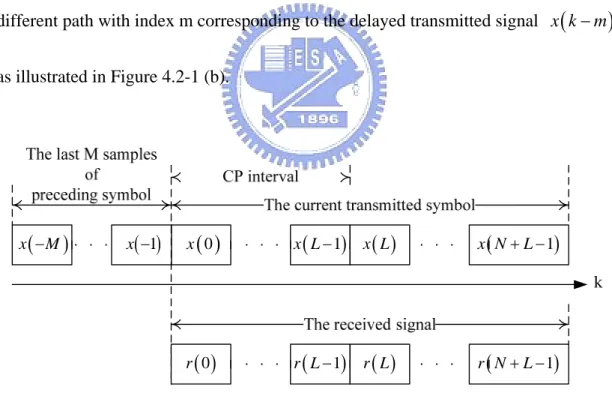
Figure 4.2-1 (a) The relation between transmitted sequence over M+1 path channel and received signal……….…59

Figure 4.2-2 M samples within CP damaged by the preceding OFDM

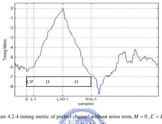
symbol…..………60 Figure 4.2-3 Proposed timing estimator………62 Figure 4.2-4 Perfect channel without noise term，M = ，0 L′ = +L D and

normalized by L′………63 Figure 4.2-5 approximates to zero within summation window

of (4.2-8) with summation window length

( ) (

)

r k −r k+D

L′………64 Figure 4.2-6 Timing metric reach to a plateau in the interval

(M=0) ………...………64 1

L′ − ≤ ≤ + −1k L D

Figure 4.3.1-1(a) Mean in AWGN channel for the case(L′=160,d =1)、

(L′=148,d = )、13 L′=128,d =33)………66 Figure 4.3.1-1(b) MSE in AWGN channel for the case(L′=160,d =1)、

(L′=148,d = )、(13 L′=128,d =33)………67 Figure 4.3.2-1(a) Mean in SUI3 channel with f_d =222.22Hz for the case

(L′=160,d = )、(1 L′=154,d = )、(1 L′=148, )、 ( , 1 d = 128 L′= d =21)………..……68 Figure 4.3.2-1(b) MSE in SUI3 channel with f_d =222.22Hz for the case

(L′=160,d = ),(1 L′=154,d = ),(1 L′=148,d = ) 1

&(L′=128,d =21)………..69 Figure 4.3.3-1(a) Mean in static SUI3 channel for the case

(L′=160,d = ),(1 L′=154,d = ),(1 L′=148,d = ) 1

&(L′=128,d =21)………....……71 Figure 4.3.3-1(b) MSE in static SUI3 channel for the case

(L′=160,d = ),(1 L′=154,d = ),(1 L′=148,d = ) 1

Figure 4.4-1(a) Mean comparison in AWGN channel……….73

Figure 4.4-1(a) MSE comparison in AWGN channel………..73

Figure 4.4-2(a) Mean comparison in mobile SUI3 with fd=222.22Hz………74

Figure 4.4-2(b) MSE comparison in mobile SUI3 with fd=222.22Hz……….74

Figure 4.4-3(a) Mean comparison in static SUI3 Channel………….……….75

Figure 4.4-3(b) MSE comparison in static SUI3 Channel………….………..75

Figure 4.4.1-1 The simulation frame structure in the downlink mode……….78

Figure 4.4.1-2 (a) Mean comparison in mobile SUI2 with fd=222.22Hz in downlink mode………...79

Figure 4.4.1-2 (b) MSE comparison in mobile SUI2 with fd=222.22Hz in downlink mode………...79

Figure 4.4.1-3 (a) Mean comparison in mobile SUI2 with fd=111.11Hz in downlink mode………...80

Figure 4.4.1-3 (b) MSE comparison in mobile SUI2 with fd=111.11Hz in downlink mode………...80

Figure 4.4.1-4 (a) Mean comparison in mobile SUI2 with fd=55.55Hz in downlink mode………...……81

Figure 4.4.1-4 (b) MSE comparison in mobile SUI2 with fd=55.55Hz in downlink mode………...…………81

Figure 4.4.1-5 (a) Mean comparison in mobile SUI3 with fd=222.22Hz in downlink mode………...82

Figure 4.4.1-5 (b) Mean comparison in mobile SUI3 with fd=222.22Hz in downlink mode……….………..82

Figure 4.4.1-6 (a) Mean comparison in mobile SUI3 with fd=111.11Hz in downlink mode………...83

Figure 4.4.1-6 (b) MSE comparison in mobile SUI3 with fd=111.11Hz in downlink mode………...83

Figure 4.4.1-7 (a) Mean comparison in mobile SUI3 with fd=55.55Hz in downlink mode...………84

Figure 4.4.1-7 (b) MSE comparison in mobile SUI3 with fd=55.55Hz in downlink mode………...84

Figure 4.4.2-1 The simulation frame structure in the uplink mode………..85 Figure 4.4.2-2 (a) Mean comparison in mobile SUI2 with fd=222.22Hz in uplink

mode………...86 Figure 4.4.2-2 (b) MSE comparison in mobile SUI2 with fd=222.22Hz in uplink

mode………...86 Figure 4.4.2-3 (a) Mean comparison in mobile SUI2 with fd=111.11Hz in uplink

mode………...…87 Figure 4.4.2-3 (b) MSE comparison in mobile SUI2 with fd=111.11Hz in uplink

mode……….………..87 Figure 4.4.2-4 (a) Mean comparison in mobile SUI2 with fd=55.55Hz in uplink

mode………...88 Figure 4.4.2-4 (b) MSE comparison in mobile SUI2 with fd=55.55Hz in uplink

mode………...88 Figure 4.4.2-5 (a) Mean comparison in mobile SUI3 with fd=222.22Hz in uplink

mode………...89 Figure 4.4.2-5 (b) MSE comparison in mobile SUI3 with fd=222.22Hz in uplink

mode………...89 Figure 4.4.2-6 (a) Mean comparison in mobile SUI3 with fd=111.11Hz in uplink

mode………...90 Figure 4.4.2-6 (b) MSE comparison in mobile SUI3 with fd=111.11Hz in uplink

mode………...90 Figure 4.4.2-7 (a) Mean comparison in mobile SUI3 with fd=55.55Hz in uplink

mode……….. 91 Figure 4.4.2-7 (b) Mean comparison in mobile SUI3 with fd=55.55Hz in uplink

List of Tables

Table 3.2.2-1 OFDM symbol parameters……….………31 Table 3.2.4-2 The inner convolutional code with puncturing configuration………35 Table 3.2.4-3 Mandatory channel coding per modulation………36 Table 3.2.5-1 Block sizes of the Bit Interleaver………37 Table 3.3-1 Simulation Parameters……….…………47 Table 3.4-1 Table 3.4-1 Terrain type for different SUI channel and with its delay

spread………...…………48 Table 3.4-2 SUI 3 channel model for BW=10 MHz………...…48 Table 3.4-3 SUI 2 channel model for BW=10 MHz………...49

Chapter 1 Introduction

Orthogonal Frequency Division Multiplexing (OFDM) is a technique that has a

high bandwidth efficiency in signaling for high-speed wireless communication

system .OFDM is more robust against frequency selective fading by inserting a guard

interval in a frame.

OFDM technology has been applied in many digital transmission systems such

as digital audio broadcasting(DAB) system , digital video broadcasting terrestrial TV

system(DVB-T),wireless local area network(WLAN) and broadband wireless

access(BWA)network.

However , an OFDM system is very sensitive to the non-ideal synchronization

parameters , such as timing offset,carrier frequency offset,sampling frequency

offset.In this thesis,we focus on the issues of timing offset (timing synchronization )

estimation.A symbol timing error will both introduce inter carrier interference(ICI)

and inter symbol interference(ISI), ISI and ICI effect may dramatically degrade the

system performance.Hence,an estimation used to extract a frame timing precisely is

necessary,because of a frame timing error results in a timing error in each symbol

within the frame.

This thesis is organized as follows.In Chapter 2,we demonstrate the essential

In Chapter 4,we review the conventional frame synchronization algorithm [4] and

present the proposed method. We also show computer simulation results and

comparisons of the performance of synchronization algorithms. Finally ,a conclusion

Chapter 2 OFDM Overview

Figure 2 OFDM Transmission System

Multicarrier modulation systems have been employed in military applications

since the 1950s.The concept of using parallel data transmission and orthogonal

frequency division multiplexing was published in early 1970s.Discrete Fourier

transform(DFT) which can be practically implemented with fast Fourier transform

(FFT) ,was applied to perform modulation and demodulation in order to eliminate the

need of banks of subcarrier oscillator and demodulator. A key improvement to OFDM

is adding cyclic prefix in the guard time interval in order to maintain the signal

orthogonality over the dispersive channels. Thus,even relatively complex OFDM

transmission systems with high data-rates are technically feasible.Now,the OFDM

modulation scheme has matured and become a well-established technology.Figure 2

2.1 Principle of OFDM Transmission [1]

For the purpose of enhancing the data transmission rate,the idea of using different

frequency band to parallelly transmit data in parallel is presented.In traditional

frequency division multiplexing(FDM) systems,the total frequency band is divided

into N non-overlapping subcarriers to avoid inter carrier interference(ICI).Because of

these spectrum are non-overlapped for FDM system,we can design a filter to

demodulate each subcarrier at the receiver side. In this case, it is not efficient in terms

of utilization of available spectrum bandwidth. However, the available spectrum

bandwidth can be used much more efficiently if the individual subcarriers are allowed

to overlap.If the frequency spacing between signal in adjacent bands is ,then the

total bandwidth in a FDM system with N sub-carriers needs

f

Δ

f NΔ

2 or more as

illustrated in Figure 2.1-1.But in an OFDM system with N subcarriers,the total

bandwidth needed is

(

N−1

)

Δf +2Δf =

(

N+1

)

Δf , which is more efficient than the conventional FDM system as shown in Figure 2.1-2.

Figure 2.1-1 The spectra of a FDM system

Figure 2.1-2 The spectra of an OFDM system

c f f_c + 4Δf f fc − 4Δ f fc − 8Δ fc + 8Δf f Δ 2 f Δ f f_c − 4Δ f_c f_c + 4Δf f f_c − 2Δ f_c + 2Δf

In the OFDM system,the serial data stream defined as input is rearranged into

a sequence of N QAM symbols at baseband.The time

duration between two QAM symbols is (where symbol rate is

( ) (

0 1 1

)

d k k= , ,_L, N -s T s s T f = 1 ),

At the k-th QAM symbol instant,the complex form of QAM symbol is

represented by an in-phase component

( )

k d

( )

k

d_I and a quadrature-phase component ,i.e. .A block of N QAM symbols are applied to a serial

to parallel converter simultaneously .There are N pairs of balanced modulators which

modulate each pair of QAM symbols, respectively . For example , the in-phase and

the quadrature-phase components ,

( )

k

dQ d

( )

k =dI

( )

k + j⋅dQ

( )

k

( )

k

d_I and dQ

( )

k , of a QAM symbols are

modulated by quadrature carriers ,cos

(

2πf_kt

)

andsin

(

2πf_kt

)

, respectively.Notice that the symbol interval of the subcarriers in the parallel system is N times longer than that

of the serial system giving that T = N⋅T_s ,which corresponds to an N-times lower symbol rate.The sub-carriers frequencies , f_k = f_c +k⋅Δf , are spaced apart by

T f = 1

( )

0 I d

( )

0 Q d

(

2 f₀t

)

cos π

(

2 f₀t

)

sin π −

( )

k d

( )

k d

( )

k d = _I + _Q

(

N−1

)

dI

(

N−1

)

dQ

(

2 f_{N 1}t

)

cos π ₋

(

2 f_{N 1}t

)

sin ₋ − π

Figure 2.1-3 Conventional OFDM transmitter at passband

Figure 2.1-4 Conventional equivalent complex baseband OFDM transmitter

Figure 2.1-3 depicts that an OFDM signal is contructed by the summation of

modulated carriers, that is ,D t_k

( )

=d_I

( ) (

k cos 2π f t_k

)

−d_Q

( ) (

k sin 2π f t_k

)

with different index k, where .Thus,we have N QAM symbols at RF,where

the k-th QAM symbol at RF is given by ： 1 1

0,, ,N-k = _L

( )

( ) (

)

( ) (

)

( )

{

}

( )

{

}

2 2 2 cos 2 sin 2 Re Re c c k I k Q j f t j k ft j f t k D t d k f t d k f t d k e e x t e π π π π π Δ = − = = k (2.1-1)

in (2.1-1) is an eqivalent complex representation for an OFDM signal at

baseband is shown in Figure 2.1-4,where the real and imaginary parts

correspond to the in-phase and quadrature-phase parts of OFDM signal,which have to

be multiplied by a cosine and a sine of the desired carrier frequency ,respectively,to

produce the final OFDM signal.By adding the outputs of each subcarrier

whose carrier frequency are offset by

( )

t x_k

( )

t x_k

( )

t x_k T f = 1

Δ ,we obtain the OFDM signal as

( )

( )

( )

k e d t x t x N-k ft k j N-k k

∑

∑

= Δ = = = 1 0 2 1 0 π T t , T t , ≤ ≤ ≤ ≤ 0 0

( )

( )

∑

= Δ _⋅ ⋅ = 1 0 2 N-k ft k j t u e k d π where

( )

(2.1-2) ⎩ ⎨ ⎧ ≤ ≤ = 0 0 1 elsewhere T t t u

∑

( ) ( )

= ⋅ = 1 0 N-k k t g k d

where ,as shown in Figure 2.1-5.In Figure 2.1-5 , designates

the transmitter filter impulse response.

( )

t e u

( )

t

( )t g₀ ( )0 d ( )t g1 ( )1 d ( )t g_k ( )k d ( )t gN 1− (N−1) d ( )t g* 1 ( )t g k * ( )t g N * 1 − ( )t g* 0 ( )0 ˆ d ( )1 ˆ d ( )k dˆ ( 1) ˆ _N− d

Figure 2.1-5 OFDM transmission model

This set of N QAM signals are transmitted simultaneously over the mobile radio

channel.At the receiver,the OFDM signal is de-multiplexed using a bank of N filters

to regenerate the N QAM signals.Because of the rectangular pulse shaping,the

spectrum of each subcarrier is a sinc function and is formulated as follows：

( )

{

( )

}

(

₍

(

₎

)

)

(

j T

(

f f f f T f f T c T t g F f G_{k k} −Δ Δ −

))

Δ − = = π π π exp sin (2.1-3)

Hence,the spectrum of an OFDM signal is constituted by the spectrum of all

subcarriers which overlap in the adjacent bands.It is shown in Figure 2.1-2.

It can seen that if the block size N is getting larger,we need a larger number of

subcarrier modems.The cost for the subcarrier modems is very high and also difficult

A discrete-time baseband model of OFDM is needed for digital implementation.It can

be shown mathematically that taking the inverse discrete Fourier transform (IDFT) of

the original block of N QAM symbols .Then transmitting the IDFT coefficients

serially is exactly equivalent to the operations required by the OFDM transmitter

employing a bank of N transmitted filter.

The total bandwidth of the OFDM system is B=N⋅Δf .The signal can be reconstructed by the complex samples at the time instant

N T n t = ⋅ with sampling period N T B t_sampling = =

Δ 1 .According to (2.1-2),the samples of the signal waveform

can be written as

( )

∑

− = ⎟ ⎠ ⎞ ⎜ ⎝ ⎛ = 1 0 2 exp N k n N n k j k d x π (2.1-4)

This equation is equivalent to IDFT of d

( )

k and shown in Figure 2.1-6.

( )

k

d

( )

0

d

( )

1

d

( )

N

−

1

d

0

x

1

x

1 − N

x

In practice,IDFT can be implemented efficientlly by inverse fast Fourier

transform (IFFT) at the transmitter side.The computation complexity of IFFT can be

reduced from to or less.Since the receiver performs the inverse

operation of transmitter,so a discrete Fourier transform (DFT) is needed at the

receiver side.DFT also can be implemented efficientlly by fast Fourier transform

(FFT).

2

N N logN

A bank of subcarrier modems are implemented using the computationally

efficient pair of inverse fast Fourier transform and fast Fourier transform (IFFT/FFT).

FFT and IFFT are defined by

1 , , 1 , 0 2 exp 1 0 − = ⎟ ⎠ ⎞ ⎜ ⎝ ⎛− =

∑

− = N k N n k j x X N n n k π L (2.1-5) 1 , , 1 , 0 2 exp 1 0 − = ⎟ ⎠ ⎞ ⎜ ⎝ ⎛ =

∑

− = N n N n k j X x N k k n π L (2.1-6)

2.2 Pilot and Vitual Carriers

In practice,some of subcarriers are allocated to carry already known data and

some of subcarriers are allocated to carry nothing in the window before IDFT

operation.These subcarriers carrying already known data are named pilots,and

subcarriers carrying nothing are named virtual subcarriers.The purpose we exploit the

two types of speciall subcarriers will be explained in the following .

There is necessity of dynamic channel estimation before demodulation of received

OFDM signal,since the wireless communication channel is time-varying and

time-dispersive.Usually,there are two types of arrangement for pilot insertion:

Comb-type and Block-type.

Figure 2.2-1 (b) Comb-Type pilot insertion

For Block-type arrangement,the pilots are inserted into all of the subcarriers of an

OFDM symbol called pilot symbol .These pilot symbols are sent peroidiclly among

the transmitted OFDM symbols.Because these pilot symbols were sent with a specific

period,it is suitable for the following condition ：if the Doppler spread of channel is

,the specificed period should be less than the coherent time

d f Δtp d f 1 ,i.e, d p f t < 1 Δ .

For Comb-Type arrangement,pilots are inserted in some specified subcarriers in

each OFDM symbol.These subcarriers carrying pilot informations are called pilot

tones.In order to estimate the channel for the subcarriers not carrying pilot

information,it needs an efficient interpolation technique.But Comb-type arrangement

is more suitable than Block-type arrangement for flat fading channel and fast fading

channel,because Comb-type arrangement has pilot informations for each transmitted

pilot tones ,Δfp,should be less than the coherent bandwidth max 1 τ ,i.e. max 1 τ < Δfp . k X− 1 − X 0 X 1 X k X 0 X 1 X k X 1 − X k X−

{ }

Xk X

Figure 2.2-2 The modulated sequence are added virtual carriers

Some subcarriers without carying any data information are called virtual

subcarriers.The reason for using zero padding is that the spectra of OFDM signals are

not strictly bandlimited ,there still exits large out-of-band energy.Adding zeros as a

guard band would decrease the energy spread to adjacent frequency bands which are

allocated for other wireless communication systems.It also could avoid aliasing.If

there are 2K+1 modulation variables,such as

{ }

X_k =

{

X_−k,_L,X₋₁,X₀,X₁,_L,X_k

}

, then

{ }

X_k are padded zero as a guard band at the tail of

{ }

X_k .Since the index of IFFT input is from 0 to N-1,the input X of IFFT becomes

{

0, 1, , ,0, ,0, − , , −1

}

= X X _L X_{k L} X _{k L} X

X

2.3 Cyclic Prefix

Due to the multipath propagation,the OFDM symbol may be interfered by

previous OFDM symbol .This phenomenon is called inter symbol interference

(ISI).To eliminate the effect of ISI,a guard interval is inserted before the OFDM

symbol.This is also one of the reasons and characteristics that OFDM system is robust

for multipath fading channel.

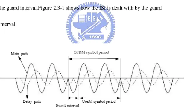
Generally,the length of guard interval should be longer than the root-mean-square

(RMS) delay spread of the channel so that ISI only damages the information within

the guard interval.Figure 2.3-1 shows how the ISI is dealt with by the guard

Interval.

Figure 2.3-1 An example of a subcarrier signal in two-ray multipath channel

The component of guard interval is the duplicate of the last data in an OFDM

symbol block,hence it is named Cyclic Prefix (CP).An OFDM frame diagram with CP

received OFDM siganl may contain the delayed by itself.We would like to

demodulate by FFT operation.However,the result of FFT operation could be exact

because of the orthogonality among each subcarrier,like the case in Figure 2.3-3 (a).

g T time interval guard within samples L u T time interval guard within samples N s T CP included symbol OFDM an of time total the

Figure 2.3-2 An OFDM symbol diagram with CP

CP

FFT window

CP

Path1

Path2

Figure 2.3-3 (a) Two-ray multipath effect without ISI

Noticing that the component of guard interval can not be inserted with zeros.If

we insert zeros within guard interval,then system performance will degrade seriously

after DFT operation.This is because there will lose orthogonality between zero

information and each component of subcarrier.Hence inserting zero information will

introduce inter carrier interference (ICI) during the process of DFT.

The case in Figure 2.3-3 (b) shows that ISI and ICI are introduced.

The channel is modeled as a discrete-time time-invariant system with finite-length

impulse response,ie.：

[ ]

[ ]

0 , 0 0 , g h n n N h n elsewhere ⎧ ≠ ≤ ≤ ⎪ ⎨ = ⎪⎩ ,

The transmitted OFDM signal is given by

[ ]

_{[ ]}

[ ]

, 0

[ ] [

]

, 0 , g g g t g g g x n n N where x n x n N n x n x n N n N N ⎧ ≤ < = + ≤ < ⎪ = ⎨ ≤ ≤ + ⎪⎩ N

and the received OFDM signal without noise is obtained as

[ ]

_{[ ] [ ]}

[ ] [ ]

, 0 , g g r h g g h x n h n n N N x n x n h n N n N N N ⎧ ⊗ ≤ < + ⎪ = ⎨ ⊗ ≤ ≤ + ⎪⎩ + Then

[ ] [ ]

, 0 g g h x n ⊗h n ≤ <n N +N is equal to x n

[ ] [ ]

⊗h n ,N+N_g ≤ ≤ +n N N_g + N k kH X

[ ]

n x h

[ ]

n

After removing the cyclic prefix,the linear convolution of the useful transmitted

The time domain channel effect could be transformed into a multiplicative

effect when demodulating by DFT at the receiver..It is shown that only simple

channel estimation and equalization is needed.

In summary,the cyclic prefixed guard interval not only preserves the mutual

orthogonality between subcarriers but also prevents the ISI between adjacent

2.4 Time and Frequency Offset

At receiver side,OFDM sysytem must operate the inverse process of the

transmitter side.Hence we have to determine the arrival time of an OFDM symbol’s

start point in order to capture the most suitable samples in a window for FFT

operation.Since timing errors may introduce both inter carrier interference(ICI) and

inter symbol interference(ISI),the OFDM system that has synchronization problem

may dramatically degrade the system performance. Timing offset is defined in Figure

2.4-1 (a) & (b).

i

offset

Timing θ

Figure 2.4-1 (a) Timing offset inside CP

1 -i

offset

Timing θ Timingoffset θ_i+1

In discrete-time baseband model,timing offset can be modeled as an integral delay

θ,so the received signal y

( )

n can be easily expressed as x

(

n−θ

)

.If θ is less than the CP length as shown in Figure 2.4-1 (a),the received signal is then given by

( )

n x

[

(

n

)

N

y = −θ

]

.Because of the circular shift property of DFT,the received signal after DFT ,Y_k, in frequency domain is given by

⎟ ⎠ ⎞ ⎜ ⎝ ⎛ = N X Y_{k k}exp 2πθ (2.4-1)

It can be easily explained as the follows. The constellation is a phase rotation if

timing offset is less than the CP length , as illustrated in Figure 2.4-3.However,if

timing offset exceeds the CP length as shown in Figure 2.4-1 (b),then ISI and ICI

occur and the system performance degrades seriously , as shown in Figure 2.4-4.

Figure 2.4-3 Timing offset is less than CP

The frequency difference of the oscilators in transmitter and receiver will result in

the frequency offset,which leads to ICI caused by the loss of orthogonality between

subcarriers , as shown in Figure 2.4-5.

' f

Figure 2.4-5 Sampling OFDM siganl with a frequency offset or not

The solid black lines in Figure 2.4-5 show the perfect synchronized position in

frequency domain.Sampling at these positions of solid black lines will not introduce

ICI and can maintain orthogonality with each subcarrier.If there is frequency offset

illustrated by solid red lines,then an offset occurs when comparing with the solid

black lines.In the descrete-time baseband model,the effect of frequency offset

between two oscillators in the transmitter and receiver can be modelled as ' f ⎟ ⎠ ⎞ ⎜ ⎝ ⎛ N k j2π ε

exp ,where ε is the ratio of the real frequency offset to the intercarrier spacing,i.e.

f f

Δ = '

and can be represented as

(

)

⎟ ⎠ ⎞ ⎜ ⎝ ⎛ = ⎟ ⎠ ⎞ ⎜ ⎝ ⎛ + =

∑

− = N n j x N k n j X N y _n K K k k n ε π ε π 2 exp 2 exp 1 ,n=0,_L,N −1,N ≥ K2 +1 (2.4-2)

where the channel effect and the noise term are ignored.

After the DFT operation,we have

_{k k}

(

( )

( )

)

(

j

(

N

)

N

)

I_k N N X Y = exp −1 + sin sin _πε πε πε ,(2.4.3) where

( )

(

)

(

)

(

N l k N

)

(

j

(

N

)

N

)

(

j

(

l k

)

N

)

X I K k l K l l k − − − ⎭ ⎬ ⎫ ⎩ ⎨ ⎧ + − =

∑

≠− = π πε ε π πε exp 1 exp sin sin .

From (2.4.3),we can see that experiences an amplitude reduction and phase shift.

is the ICI term caused by frequency offset.

k

X

k

I

It can be seen in Figure 2.4-6 and 2.4-7 that the constellation is only rotated by a

small angele under small frequency offset,but the constellation is distored and can not

Figure 2.4-6 The contellation is influenced by a small frequency offset

Chapter 3

IEEE 802.16e WiMax

Worldwide Interoperability for Microwave Access(WiMax) is the common name

associated to IEEE 802.16a/d/e standards.

These standards are issued by the IEEE 802.16 subgroup that originally covered the

Wireless Local Loop technologies with radio spectrum from 10 to 66 GHz.

According to the different locations of subscriber station (SS) and to avoid the

interference from the other base station on SS,the modulation and coding schemes

may be adjusted individually to each subscriber station (SS) on a burst-by-burst basis,

as illustrated by Figure 3.

For downlink(DL) transmission,multiple SSs can associate the same downlink burst;

and for uplink(UL) transmission,SS transmits in an given time slot with a specific

burst.

3.1 IEEE 802.16

IEEE 802.16 standard is for Line-of-Sight (LOS) applications utilizing 10-66

Ghz spectrum. Although this spectral range has a severe atmospheric attenuation, it is

suitable for connections in the operator network between two nodes with high

amounts of bandwidth because many base stations are deployed at elevated positions

from the ground. This is not suitable for residential settings because of the

Non-Line-of-Sight (NLOS) characteristics caused by rooftops or trees.

IEEE 802.16a is an amendment for NLOS utilizing 2-11Ghz,which is good for

Point-to-Multipoint(PMP) and home application.Orthogonal Frequency Division

Multiplexing(OFDM) is adopted for transmission.

IEEE 802.16-2004 revises and replaces 802.16,802.16a,and 802.16REVd. This is

the completion of the essential fixed wireless standard.Some operators are already

interested in integrating this with the Cellular backhaul.After some political debates,it

was decided to support not mobile but fixed wireless and nomadic

communications.Nomadicity is this: Users are attached to the network.After a session

completes,they can move to a different network.But the session should be

re-established (possibly including the authentication) from scratch;；it does not have a

hand-off mechanism.

communications at vehicular speeds.This supports a full hand-off.A user’s session is

3.2 OFDM PHY Specification

3.2.1 Time and Frequency Description of OFDM

The WirelessMAN-OFDM PHY is based on OFDM modulation and designed

for NLOS operation in the frequency bands below 11 GHz.

The transmitter energy increases with the length of the guard interval while the

receiver energy remains the same (the cyclic extension is discarded).Thus there is a

( )

10 log 1 log 10 g g b T T T ⎛ ⎞ − ⎜ ⎟ ⎜ ₊ ⎟ ⎝ ⎠ _{dB loss in} 0 b E N .

On initialization,an SS should search all possible values of CP until it finds the

CP being used by the BS.The SS shall use the same CP on the uplink. Once a specific

CP duration has been selected by the BS for operation on the downlink, it should not

be changed.Changing the CP would force all the SSs to resynchronize to the BS.

Figure 3.2-1 illustrates the time structure of OFDM symbol ,while Figure 3.2-2

gives a frequency description of OFDM signals.

Figure 3.2.1-2 OFDM frequency description

Data sub-carriers：For data transmission.

Pilot- subcarriers：For various estimation purposes.

Null- subcarriers： No transmission at all, for guard bands, non-active subcarriers and the DC subcarrier.

3.2.2 Parameter Setting

(a) Primitive parameter definitions：

– BW ： This is the nominal channel bandwidth. – N_used： Number of used subcarriers.

– n：Sampling factor. This parameter, in conjunction with BW and N_used determines the subcarrier spacing, and the useful symbol time.

– G： This is the ratio of CP time to “useful” time.

(b) Derived parameter definitions ：

– N_FFT：Smallest power of two greater than N_used.

– Sampling Frequency：

(

)

8000

8000

s n BW

F = floor ⋅ × – Subcarrier spacing ：Δ =f F N_{s FFT}

– Useful symbol time： T_b = Δ 1 f – CP Time： T_g = ⋅G T_b

– OFDM Symbol Time：T_s =T_b+T_g – Sampling time：T N_{b FFT}

(c) Table 3.2.2-1 gives the OFDM Symbol parameters

Parameter Value

u sed F F T

N

N

200/256

G 1 4 , 1 8 , 1 16 , 1 32

Frequency offset indices of pilot

carriers –88,–63,–38,–13,13,38,63,88 Frequency offset indices of guard

subcarriers

–128,–127...,–101 (numbers：28) +101,+102,...,127 (numbers：27)

n

For channel bandwidths that are a multiple of {1.75 MHz then n = 8/7 1.5 MHz then n = 86/75 1.25 MHz then n = 144/125 2.75 MHz then n = 316/275 2.0 MHz then n = 57/50

otherwise specified then n = 8/7} Table 3.2.2-1 OFDM symbol parameters

3.2.3

Randomization of Data

A Pseudo Random Binary Sequence(PRBS) generator is shown in Figure 3.2.3-1

Data randomization is performed on each burst of data on the downlink and

uplink.The randomization is performed on each allocation (downlink or

uplink),which means that for each allocation of a data block (subchannels on the

frequency domain and OFDM symbols on the time domain) the randomizer shall

be used independently.If the amount of data to transmit does not fit exactly the

amount of data allocated,padding of 0xFF (“1” only) shall be added to the end of

the transmission block for the unused integer bytes. For RS-CC and CC encoded

data,,padding will be added to the end of the transmission block, up to the

amount of data allocated minus one byte,which shall be reserved for the

introduction of a 0x00 tail byte by the FEC.

On the downlink, the randomizer shall be re-initialized at the start of each frame

with the sequence: 1 0 0 1 0 1 0 1 0 0 0 0 0 0 0. The randomizer shall not be reset at

the start of burst #1. At the start of subsequent bursts,the randomizer shall be

initialized with the vector shown in Figure 3.2.3-2.

Figure 3.2.3-2 OFDM randomizer downlink initialization vector for burst #2...N

On the uplink,the randomizer is initialized with the vector shown in Figure

3.2.3-3.The frame number used for initialization is that of the frame in which the UL

map that specifies the uplink burst was transmitted.

3.2.4

FEC

A Forward Error-Correction code(FEC),consisting of the concatenation of a

Reed–Solomon outer code and a rate-compatible convolutional inner code, shall be

supported on both uplink and downlink. Support of Block Turbo Code(BTC) and

Convolutional Turbo Code (CTC) is optional.

The most robust burst profile shall always be used as the coding mode when

requesting access to the network and in the FCH burst.The encoding is performed by

first passing the data in block format through the RS encoder and then passing it

through a zero-terminating convolutional encoder.

The Reed–Solomon encoding shall be derived from a systematic RS (N = 255, K =

239, T = 8) code.Puncturing patterns and serialization order that shall be used to

realize different code rates are defined in Table 3.2.4-2. In the table,“1” means a

transmitted bit and “0” denotes a removed bit, whereas X and Y are in reference to

Figure 3.2.4-1 Convolutional encoder of rate 1/2

Table 3.2.4-2 The inner convolutional code with puncturing configuration

Table 3.2-4-3 gives the block sizes and the code rates used for the different

modulations and code rates. As 64-QAM is optional for license-exempt bands, the

codes for this modulation shall only be implemented if the modulation is

Table 3.2.4-3 Mandatory channel coding per modulation

When subchannelization is applied, the FEC shall bypass the RS encoder and

use the Overall Coding Rate as indicated in Table 3.2.4-3 as CC Code Rate.The

Uncoded Block Size and Coded Block size may be computed by multiplying the

values listed in Table 3.2.4-3 by the number of allocated subchannels divided by 16.

3.2-5

Interleaving

All encoded data bits shall be interleaved by a block interleaver with a block size

corresponding to the number of coded bits per the allocated subchannels per OFDM

symbol,Ncbps.Table 3.2-5-1 gives the block size of the Bit Interleaver.

3.2.6 Modulation

After bit interleaving,the data bits are entered serially to the constellation

mapper.BPSK,Gray-mapped QPSK,16-QAM,and 64-QAM as shown in Figure

3.2-6-1 shall be supported,whereas the support of 64-QAM is optional for

license-exempt bands.The constellations (as shown in Figure 3.2-6-1) shall be

normalized by multiplying the constellation point with the indicated factor c to

achieve equal average power.For each modulation, b0 denotes the least significant bit

(LSB).

The constellation-mapped data shall be subsequently modulated onto all

allocated data subcarriers in order of increasing frequency offset index.The first

symbol out of the data constellation mapping shall be modulated onto the allocated

3.2.7

Pilot Modulation

Pilot subcarriers shall be inserted into each data burst in order to constitute the

symbol and they shall be modulated according to their carrier location within the

OFDM symbol. The PRBS generator depicted hereafter shall be used to produce a

sequence, w .The polynomial for the PRBS generator shall be _k X11+X9+ . 1

The value of the pilot modulation for OFDM symbol k is derived from wk. On

the downlink ,the index k represents the symbol index relative to the beginning of the

downlink subframe. For bursts contained in the STC zone when the FCH-STC is

present,index k represents the symbol index relative to the beginning of the STC zone.

In the DL Subchannelization Zone,the index k represents the symbol index relative to

the beginning of the burst.On the uplink ,the index k represents the symbol index

relative to the beginning of the burst.On both uplink and downlink,the first symbol of

the preamble is denoted by k=0.The initialization sequences that shall be used on the

downlink and uplink are shown in Figure 3.2-7-1.On the downlink,this shall result in

the sequence 11111111111000000000110… where the 3rd 1, i.e.,w2 =1,shall be used

in the first OFDM downlink symbol following the frame preamble.For each pilot

(indicated by frequency offset index),the BPSK modulation shall be derived as

DL: c₋₈₈ =c₋₃₈ =c₆₃ =c₈₈ =1−2w_k and c₋₆₃ =c₋₁₃ =c₁₃ =c₃₈ =1−2w_k UL: c₋₈₈ =c₋₃₈ =c₁₃ =c₃₈ =c₆₃ =c₈₈ =1−2w_k and c₋₆₃ =c₋₁₃ =1−2w_k

3.2.8 Preamble structure

The first preamble in the downlink PHY PDU,as well as the initial ranging

preamble,consists of two consecutive OFDM symbols.The first OFDM symbol uses

only subcarriers the indices of which are a multiple of 4.As a result, the time domain

waveform of the first symbol consists of four repetitions of 64-sample

fragment,preceded by a CP.The second OFDM symbol utilizes only even

subcarriers,resulting in time domain structure composed of two repetitions of a

128-sample fragment,preceded by a CP.The time domain structure is exemplified in

Figure 3.2-12.This combination of the two OFDM symbols is referred to as the long

preamble.

Figure 3.2.8-1 Downlink and network entry preamble structure

The frequency domain sequences for all full-bandwidth preambles are derived from

the sequence： PALL(-100:100) = {1-j, 1-j, -1-j, 1+j, 1-j, 1-j, -1+j, 1-j, 1-j, 1-j, 1+j, -1-j, 1+j, 1+j, -1-j, 1+j, -1-j, -1-j, 1-j, -1+j, 1-j, 1-j, -1-j, 1+j, 1-j, 1-j, -1+j, 1-j, 1-j, 1-j, 1+j, -1-j, 1+j, 1+j, -1-j, 1+j, -1-j, -1-j, 1-j, -1+j, 1-j, 1-j, -1-j, 1+j, 1-j, 1-j, -1+j, 1-j, 1-j, 1-j, 1+j, -1-j, 1+j, 1+j, -1-j, 1+j, -1-j, -1-j, 1-j, -1+j, 1+j, 1+j, 1-j, -1+j, 1+j, 1+j, -1-j, 1+j, 1+j, 1+j, -1+j, 1-j, -1+j, -1+j, 1-j, -1+j, 1-j, 1-j,1+j, -1-j, -1-j, -1-j, -1+j, 1-j, -1-j, -1-j, 1+j, -1-j, -1-j, -1-j, 1-j, -1+j, 1-j, 1-j, -1+j, 1-j, -1+j,-1+j, -1-j, 1+j, 0, -1-j, 1+j, -1+j, -1+j, -1-j, 1+j, 1+j, 1+j, -1-j, 1+j, 1-j, 1-j, 1-j, -1+j, -1+j, -1+j, -1+j, 1-j, -1-j, -1-j, -1+j, 1-j, 1+j, 1+j, -1+j, 1-j, 1-j, 1-j, -1+j, 1-j, -1-j, -1-j, -1-j, 1+j,1+j, 1+j, 1+j, -1-j, -1+j, -1+j, 1+j, -1-j, 1-j, 1-j, 1+j, -1-j, -1-j, -1-j, 1+j, -1-j, -1+j, -1+j, -1+j, 1-j, 1-j, 1-j, 1-j, -1+j, 1+j, 1+j, -1-j, 1+j, -1+j, -1+j, -1-j, 1+j, 1+j, 1+j, -1-j, 1+j, 1-j, 1-j, 1-j, -1+j, -1+j, -1+j, -1+j, 1-j, -1-j, -1-j, 1-j, -1+j, -1-j, -1-j, 1-j, -1+j, -1+j, -1+j, 1-j, -1+j,1+j, 1+j, 1+j, -1-j,

-1-j, -1-j, -1-j, 1+j, 1-j, 1-j}

The frequency domain sequence for the 4 times 64 sequence P4x64 is defined by：

( )

(

( )

)

mod 4 4 64 mod 4 2 2 0 0 0 ALL conj P k k P k k × ⎧ _{⋅ ⋅ =} ⎪ = ⎨ ≠ ⎪⎩

the factor of 2 equates the Root-Mean-Square (RMS) power with that of the data

section.The additional factor of 2 is related to the 3 dB boost.

The frequency domain sequence for the 2 times 128 sequence PEVEN is defined by：

( )

(

( )

)

mod 2 mod 2 2 0 0 ALL EVEN conj P k k P k k ⎧ ⋅ =0 ⎪ = ⎨ ≠ ⎪⎩

In P_EVEN,the factor of 2 is related to the 3 dB boost.

In the uplink,when the entire 16 subchannels are used,the data preamble,as shown

in Figure 3.2.8-2 ,consists of one OFDM symbol utilizing only even subcarriers.The

time domain waveform consists of two 128 samples preceded by a CP. The subcarrier

values shall be set according to the sequence . This preamble is referred to as

the short preamble. This preamble shall be used as burst preamble on the downlink

bursts when indicated in the DL-MAP_IE.

EVEN

P

3.2.9

Frame Structure

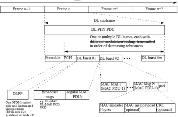
A frame consists of a downlink subframe and an uplink subframe.

(a) Time-Division Duplex(TDD) Frame structure

Figure 3.2.9-1 illustrates an example of OFDM frame structure with TDD. Downlink

– A downlink subframe consists of only one downlink PHY PDU.

– A downlink PHY PDU starts with a long preamble,which is used for PHY

synchronization.

– The FCH burst is one OFDM symbol long and is transmitted using BPSK rate

1/2 with the mandatory coding scheme.

– Each downlink burst consists of an integer number of OFDM

symbols,carrying MAC messages,i.e., MAC PDUs.

Uplink

– A uplink subframe consists of contention intervals scheduled for initial

ranging and bandwidth request purposes and one or multiple uplink PHY

PDUs,each transmitted from a different SS.

– An uplink PHY burst,consists of an integer number of OFDM

In each TDD frame (see Figure 3.2.9-1),the Tx transition gap(TTG) and Rx

transition gap (RTG) shall be inserted between the downlink and uplink subframe and

at the end of each frame,respectively,to allow the BS to turn around.

z Frequency-Division Duplex (FDD) Frame structure

Basically,the frame structure of FDD is same with the frame structure of TDD.

Figure 3.2.9-2 illustrates downlink and uplink frame structure of an OFDM system.

Figure 3.2.9-2 (a) OFDM frame structure with FDD for downlink subframe

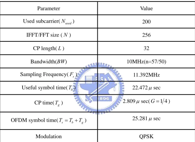
3.3 Simulation Parameter

Table 3.3-1 are the simulation parameters used for each simulation in our study

(Chapter 4).

Parameter Value Used subcarrier(N_used) 200

IFFT/FFT size (N ) 256

CP length(L) 32

Bandwidth(BW) 10MHz(n=57/50) Sampling Frequency(F ) _s 11.392MHz

Useful symbol time(T_b) 22.472μ sec CP time(T_g) 2.809μ sec(G=1 4) OFDM symbol time(T_s =T_b +T_g) 25.281μ sec

Modulation QPSK Table 3.3-1 Simulation Parameters

3.4 Channel Model

There is not a formal channel model issured for 802.16e.In this thesis we still

simulate in SUI channel but make some modifications for Doppler frequency such

that it is suitable for mobile channel.

SUI channel is proposed by Stanford University and has 3 terrain types:

(a) Terrain Type A：The maximum path loss category；hilly terrain with

moderate-to-heavy tree density.

(b) Terrain Type B：The intermediate path loss category.

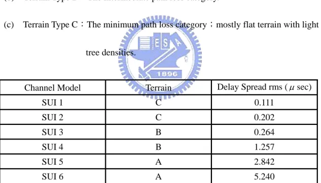
(c) Terrain Type C：The minimum path loss category；mostly flat terrain with light

tree densities.

Channel Model Terrain Delay Spread rms (μ sec)

SUI 1 C 0.111 SUI 2 C 0.202 SUI 3 B 0.264 SUI 4 B 1.257 SUI 5 A 2.842 SUI 6 A 5.240

Table 3.4-1 Terrain type for different SUI channel and with its delay spread

SUI3(10MHz) Tap power(dB) Delay samples

Tap1 0 0 Tap2 -5 6 Tap3 -10 12

SUI2(10MHz) Tap power(dB) Delay samples

Tap1 0 0 Tap2 -12 5 Tap3 -15 13

Table 3.4-3 SUI 2 channel model for BW=10 MHz

Table 3.4-1 illustrates the terrain type for different SUI channels ,while Table

3.4-2 illustrates the SUI3 channel for BW=10MHz.

SUI channel model is used for statistic environment,so it is not suit for mobile

environment.For NLOS (Non-Line-Of -Sight) transmission,the operating frequency

band is between 2~11GHZ.

If relative velocity between transmitter and receiver is =120 km/hr,we can

calculate the Doppler frequency under different operating frequency band.

v

For example：

c

f ：the carrier frequency 2 GHz

c ：velocity of light(3 10× 8m/s)

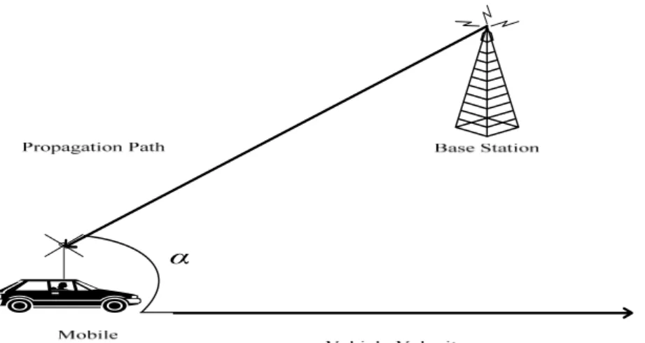
α：the angle between propagation path and direction of vehicle which is plotting in Figure 3.4-1

the definition of Doppler frequency( f ) is _d

( )

( )

( )

9 8 cos 100 2 10 cos 3 3 10 =222.22 cos Hz c d v f f c α α α ⋅ = ⋅ = ⋅ ⋅ ⋅

α

Figure 3.4-1 the angle between propagation path and direction of vehicle

Hence,for the worst case that is α = ,then 0 f =222.22Hz. _d

Next we substitute the Doppler frequency from the each path of original SUI3 or

Chapter 4 Frame Synchronization

In the transmitter,QAM signals are converted into parallel and fed to each port of

IFFT.To add the CP within guard interval in front of an OFDM symbol,the copy of

latter part of OFDM symbol is added to the symbol as a prefix and converted into

serial form for transmission.In the receiving end,received OFDM signal is converted

into parallel form and fed to FFT.Since signal is transmitted over a multipath fading

channel,the received signal is distorted by multipath delayed signals.A guard interval

is often used to reduce the effect of multipath delay spread ,so that the received signal

is distorted by the preceding symbol only within the guard interval.To demodulate the

OFDM symbol correctly,the ideal frame timing is at the end of the guard interval;

otherwise,it should be started at the timing that the signal is not disturbed by the

preceding symbol.Figure 4 illustrates process of frame synchronization .Our goal is to

estimate the start timing of a frame by timing estimator for a frame.

4.1 Overview of Schmidl & Cox Frame Synchronization

Scheme[4]

The downlink preamble structure specified in 802.16e is shown in Figure 4.1-1

which consists of two parts,referred as short preamble and long preamble.The short

preamble consists of four repeated 64-sample blocks,and the long preamble consists

of two repeated 128-sample blocks.In order to avoid inter symbol interference (ISI),

cyclic prefix (CP) is added ,respectively ,in front of short preamble and long

preamble.

Figure 4.1-1 The downlink preamble structure specified in 802.16e

One of the famous estimation methods that exploit the characteristic of preamble

for frame synchronization was proposed by Schmidl & Cox[4].This is mainly used to

estimate the start position of training symbol by using the two repeated 128-sample

blocks.In [4], a timing metric M k is defined as (4.1-3).

( )

( )

1 *

(

) (

)

0 D m P k r k m r k m D − = =

∑

+ + + (4.1-1)

( )

1

(

)

2 0 D m R k r k m D − = =

∑

+ + (4.1-2)

( )

( )

( )

(

)

2 2 P k M k R k = (4.1-3)

where k is a time index

( )

r k is the received signal at k-th sample in time domain

D is the length of the half long preamble ,D=128

( )

r k

( )

* θˆ

( )

2 2

( )

P k

( )

R k

( )

M k

Figure 4.1-2 Block diagram of estimator by [4]

2

From (4.1-1),we can imagine that a sliding window of D samples slides along

the received signals in time .This window slides as the estimator looks for the start

position of the first 128-sample block, as shown in Figure 4.1-3.

Eq.(4.1-2) defines the received energy of the second 128-sample block.

Both (4.1-1) and (4.1-2) can be implemented with the iterative formula such as

(

)

( )

*

(

) (

)

*

( ) (

)

1 2 P k+ = P k +_⎣⎡r k+D r k+ ⋅D _{⎦ ⎣}⎤ ⎡− r k r k+D ⎤⎦ (4.1-4)

(

)

( ) (

)

2

(

)

1 2 R k+ =R k + r k+ ⋅D − r k+D 2 (4.1-5)

Figure 4.1-3 A sliding window slides to the different position in time domain for searching the first 128-sample block

Noting that, a short preamble can also be regarded as a preamble with two

identical halves in time domain.The transmitted long preamble signal is received as a

consecutive sequence and calculated by (4.1-1) & (4.1-2).From Figure 4.1-3,if

channel is non-time-dispersive,then CP is not damaged.Thus,when the first point of

the sliding window is within the interval of CP,then the first half of sliding window is

identical to the second half, until the first point of the sliding window is outside the

interval of CP.

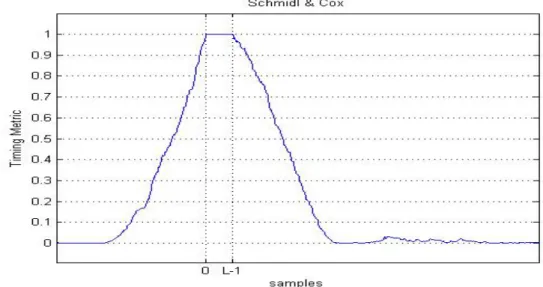
Hence,this gives the result that the timing metric will reach to a plateau which

starts at the first point of CP and ends at the last point of CP.This plateau has a length

equal to the length of guard interval in AWGN channel,as shown in the Figure 4.1-4

Figure 4.1-4 The timing metric has the length of plateau is L

If there is ISI effect which distorts OFDM signal in the front part of guard

interval,then the plateau length is equal to the length of guard interval minus the

length of the channel impulse response.Because we take the undistorted signal

( )

r k within guard interval to calculate the correlation with the delay signal

over a summation range with its size equal to

(

)

r k+D D ,the result of P k is a large

( )

value,until r k is outside of guard interval and not all of

( )

r k is equal to

( )

in the sliding window.The way to extract the estimated position proposed

by [4] is to find the maximum values of timing metric.

(

r k+D

)

The appearance of plateau leads some uncertainty when we want to confirm the

accurate FFT window .The extracted timing gives larger mean and variance for

transition gap in time between two transmitted frames and the first symbol of a frame

is the long preamble.

Figure 4.1-5 The simulation frame structure

In Figure 4.1-5,mean is defined as ：

(

)

F ˆ N i i i Mean θ θ− =

∑

where θ_i：the real start position at i-th frame ˆ

i

θ ：the estimated position by [4] at i-th frame

F

N ：the total numbers of frames

If mean is a negative number, it indicates that the estimated start position is too

early extracted.For a perfect estimation,we prefer the mean value approximately equal

to zero or approximates to a tolerance error in estimation.A tolerance error is that we

would like the mean to be negative and the absolute value of mean not to exceed the

length of guard interval minus the length of channel impulse response.The mean value

in Figure 4.1-5 indicates that although the method of [4] can avoid the ISI effect,it is

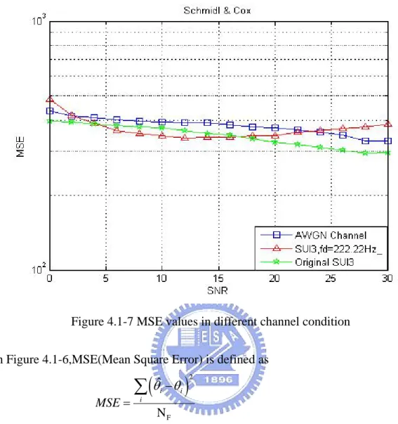
Figure 4.1-7 MSE values in different channel condition

In Figure 4.1-6,MSE(Mean Square Error) is defined as

(

)

2 F ˆ N i i i MSE θ θ− =

∑

where θ_i：the real start position at i-th frame ˆ

i

θ ：the estimated position by [4] at i-th frame

F

N ：the total numbers of frames

The MSE is still quite large indicates that this is not a precise estimation,but this

method still can work at very low signal-to-noise ratio (SNR).