用於H.264視訊解碼器之記憶體控制器與熵解碼器之設計

全文

(1)國立交通大學電子工程學系電子研究所碩士論文. 用於 H.264 視訊解碼器之記憶體控制器與熵解碼器之設計. Designs of Memory Controller and Entropy Decoder for H.264/AVC Video Decoder. 研究生：余國亘指導教授：張添烜博士. 中華民國九十五年十月.

(2) 用於 H.264 視訊解碼器之記憶體控制器與熵解碼器之設計. Designs of Memory Controller and Entropy Decoder for H.264/AVC Video Decoder 研究生：余國亘指導教授：張添烜博士 Chang. Student: Guo-Shiuan Yu Advisor: Dr. Tian-Sheuan. 國立交通大學電子工程學系電子研究所碩士論文 A Thesis Submitted to Department of Electronics Engineering & Institute of Electronics College of Electrical & Computer Engineering National Chiao Tung University in partial Fulfillment of the Requirements for the Degree of Master in Electronics Engineering & Institute of Electronics October 2006 Hsinchu, Taiwan, Republic of China. 中華民國九十五年十月.

(3) 用於 H.264 視訊解碼器之記憶體控制器與熵解碼器之設計研究生：余國亘. 指導教授：張添烜博士. 國立交通大學電子研究所. 摘要. 近年來，數位視訊科技逐漸普及並廣泛得使用在日常生活中。隨著對於更佳編碼效率的需求，H.264/AVC 被視為下一代的國際視訊編碼標準。和之前的標準相比，如：MPEG-2 和 MPEG-4，新的標準藉由各式先進編碼工具明顯降低資料量並維持相同的視訊品質。對於這些技術，特別是框外預測，視訊解碼器系統需要在有限的短時間內存取大量的資料。由於數量的龐大，視訊資料存於晶片外之記憶體，而這些記憶體通常效能較差，因此系統效能高度依賴於外部記憶體與解碼器之間的頻寬。此外熵編碼技術的可變長度編碼特性造成了另一個系統效能的瓶頸，因為在硬體設計上這很難直接運用平行化和管線化來加速。. 為了解決上述的問題，我們首先提出一個考慮到資料對應的記憶體控制器藉由要求內與要求外的最佳化，來改善外部記憶體的頻寬。結果，對於大小格式為 525SD，QP 為 20 的視訊序列，失誤率為 1.8%，而完成即時明度與彩度動態補償所需的頻寬為 46.96MBps。第二，我們設計了一個採用部份多重符號解碼，零跳躍以及跳躍式合併操作的熵編碼技術解碼器，它能夠減少需要的處理時脈，和其它已發表的 CAVLC 解碼器相比，最高可減少 76%。在硬體的成本方面，CAVLC 解 I.

(4) 碼器需要大約 11K 的邏輯閘，而 UVLC 解碼器需要 1.8K。藉由提出的兩個關鍵模組，系統效能可以被有效的提升，特別是那些需要較低功耗與較高視訊品質的應用。. II.

(5) Designs of Memory Controller and Entropy Decoder for H.264/AVC Video Decoder. Student : Guo-Shiuan Yu. Advisor: Dr. Tian-Sheuan Chang. Institute of Electronics National Chiao Tung University. Abstract. In recent years, digital video technology becomes popular and is widely used in our daily life. With demand of better coding performance, H.264/AVC is regarded as the international video coding standard for next generation. Comparing with prior video standards such as MPEG-2 and MPEG-4, the new standard achieve significant bit-rate reduction while still maintain the same video quality with various advanced coding tools. With these techniques especially for inter prediction, a large amount of data within a tightly bounded time is demanded in the video decoder system. Due to the large quantities, video data are stored in off-chip memories, that are usually slow, and thus the system performance strongly depends on the memory bandwidth between decoder and external memory. Besides, the variable length coding characteristics of entropy decoding builds another bottleneck in overall system since it is difficult to speedup the hardware design by directly applying parallelism and pipelining.. To solve above problems, we first proposed a data mapping aware memory III.

(6) controller to improve the external memory bandwidth with the optimized operation of both intra and inter request issues. As a result, the miss rate is about 1.8% for 525SD video sequence format with QP = 20 and the required bandwidth is 46.96MBps for real-time decoding of luma and chroma motion compensation. Second, a entropy decoder, which employee the techniques such as partial multi-symbol decoding, zero skipping and skipped merging operation of runs and levels, is designed to reduce the required processing cycles by up to 76% for the QP=28 case when compared with other CAVLC decoder designs. The hardware cost in gate count is about 11k for CAVLC decoder and 1.8k for UVLC decoder. With these two proposed key modules, the system performance can be greatly enhanced especially for the applications with demand of lower power consumption and higher video quality.. IV.

(7) 誌謝. 首先，我要感謝我的指導教授，張添烜博士，這兩年來給我的支持與鼓勵，研究上解決我的困難和疑問。張教授的支援讓我無後顧之憂，專心於研究，才有這本論文的產生。對此致上深深的感謝。. 同時也要謝謝我的口試委員們，交大電子李鎮宜教授和清華電機陳永昌教授，感謝教授們百忙之中抽空來指導我，各位的寶貴意見讓本論文更加完備。. 接著，感謝實驗室的夥伴們。謝謝張彥中，林佑昆和鄭朝鐘學長，給予課程和研究上的建議與指導，讓研究能順利完成。感謝蔡旻奇，吳錦木同學，在課業和研究上，陪伴我一同的學習與成長。感謝古君偉，王裕仁，與我交流硬體設計及視訊處理上的經驗和技巧。感謝海珊學長，郭子筠，林嘉俊，吳秈璟，李得瑋學弟們，和我一同渡過了實驗室的生活。凡走過的，必留下痕跡，這些，都是我寶貴的回憶。. 感謝我的家人，父母，妹妹給我的溫暖是生活的支柱。感謝京阿尼公司，stack 社，LEAF 社和 KEY 社，你們製作的產品，是我踏入視訊處理領域的肇因。最後，要謝的人太多了，那就謝天吧。. 在此，僅將本論文獻給所有愛我與我愛的人。. V.

(8) Contents. Chapter 1. INTRODUCTION ................................................................................. …1. 1.1. Motivation.................................................................................................. …1. 1.2. Thesis Organization ................................................................................... …4. Chapter 2 OVERVIEW OF H.264/AVC STANDARD… .................................... …5 2.1. Overview…................................................................................................ …5. 2.2. Video Coding Tools................................................................................... …7. 2.3. 2.2.1. Intra Frame Prediction ........................................................................ 7. 2.2.2. Inter Frame Prediction ........................................................................ 8. 2.2.3. Transform.......................................................................................... 11. 2.2.4. Quantization...................................................................................... 11. 2.2.5. Entropy Coding................................................................................. 12. 2.2.5. In-loop Deblocking Filter ................................................................. 13. Profiles ..................................................................................................... …13. Chapter 3 DATA MAPPING AWARE FRAME MEMORY CONTROLLER .. 15 3.1. 3.2. Backgrounds ................................................................................................ 15 3.1.1. Features of SDRAM ......................................................................... 15. 3.1.2. Previous Work .................................................................................. 20. 3.1.3. Problem Definition............................................................................ 21. 3.1.4. Estimation of Bandwidth Requirement............................................. 23. Optimization of Memory Access ................................................................. 27 3.2.1. Intra-request Optimization ................................................................ 27. 3.2.2. The Memory Operations In Single Request...................................... 33. 3.2.3. Burst Length Selection...................................................................... 36. VI.

(9) 3.2.4. Inter-request Optimization ................................................................ 37. 3.2.5. Overall Access Flow ......................................................................... 42. 3.2.6. Performance In Different Frame Size ............................................... 44. 3.2.7. Performance Comparison.................................................................. 46. 3.3. Hardware Architecture of Memory Controller ............................................ 49. 3.4. Summary ...................................................................................................... 53. Chapter 4 4.1. Entropy Decoder...................................................................................... 54 UVLC decoder ............................................................................................. 54 4.1.1. Syntax Organization Under Macroblock Layer................................ 56. 4.1.2 Hardware Architecture of UVLC...................................................... 61 4.2. 4.3. CAVLC decoder .......................................................................................... 63 4.2.1. Introduction....................................................................................... 63. 4.2.2. Overview of CAVLC........................................................................ 64. 4.2.3. The Proposed CAVLC Decoding Flow ............................................ 66. 4.2.4. Hardware Architecture of CAVLC Decoder .................................... 72. 4.2.5. Performance Analysis ....................................................................... 76. Summary ...................................................................................................... 78. Chapter 5. Implement Result..................................................................................... 81. Chapter 6. Conclusion ................................................................................................ 84. References...................................................................................................................... 86. VII.

(10) List of Figures. Fig.1 Basic coding structure for H.264/AVC ................................................................... 6 Fig.2 Intra 4x4 prediction modes ...................................................................................... 8 Fig.3 Inter macroblock partitions...................................................................................... 9 Fig.4 Fractional interpolation for motion compensation ................................................ 10 Fig.5 Multiple reference frame motion compensation.................................................... 11 Fig.6 Profiles................................................................................................................... 14 Fig.7 Simplified architecture of typical 4-bank SDRAM............................................... 15 Fig.8 Typical read/write accesses in SDRAM................................................................ 17 Fig.9 Random read/write access ..................................................................................... 18 Fig.10 Bank alternating read access................................................................................ 19 Fig.11 Memory access under different row miss count.................................................. 22 Fig.12 Cycles overlapped by bank interleaving technique ............................................. 22 Fig.13 Possible required area between adjacent blocks.................................................. 23 Fig.14 Reference blocks for deblocking fliter ................................................................ 25 Fig.15 Block types in H.264 ........................................................................................... 25 Fig.16 1-D row break probability model ........................................................................ 28 Fig.17 Miss rate in different row windows..................................................................... 32 Fig.18 Translation of physical location and image position ........................................... 32 Fig.19 Bank arrangement with optimization .................................................................. 33 Fig.20 Request classification .......................................................................................... 34 Fig.21 Request operations in different cases .................................................................. 35 Fig.22 Distribution of request kinds ............................................................................... 35 Fig.23 Wasted data in different data burst length ........................................................... 37 Fig.24 Memory operation under row miss and row hit .................................................. 40. VIII.

(11) Fig.25 Read/write operation in I-frame and P-frame...................................................... 41 Fig.26 Chroma data arrangement.................................................................................... 42 Fig.27 Read and write request process flow ................................................................... 44 Fig.28 Miss rate average in different frame sizes ........................................................... 45 Fig.29 Miss rate variance in different frame sizes.......................................................... 46 Fig.30 Average bandwidth under different methods ...................................................... 47 Fig.31 Memory controller design ................................................................................... 49 Fig.32 Bit arrangement in address generator .................................................................. 50 Fig.33 Scan order for 4x4 luma blocks........................................................................... 51 Fig.34 Exp-Golomb code construction ........................................................................... 53 Fig.35 Syntax organization ............................................................................................. 60 Fig.36 Architecture of UVLC decoder ........................................................................... 61 Fig.37 Typical CAVLC decoding flow .......................................................................... 64 Fig.38 Cycle count distribution in different process....................................................... 65 Fig.39 The proposed decoding flow of CAVLC ............................................................ 66 Fig.40 Proposed T1s decoding........................................................................................ 67 Fig.41 Different cases of the proposed run decoding and merging ................................ 69 Fig.42 The critical cases for CAVLC decoding design, where the X denotes the nonzero coefficients .......................................................................................... 71 Fig.43 The proposed architectures for CAVLC decoding .............................................. 72 Fig.44 Architecture of coeff_token-sign decoder ........................................................... 73 Fig.45 The architecture of coefficient merging unit ....................................................... 75. IX.

(12) List of Tables. Table 1 SDRAM timing characteristics.......................................................................... 20 Table 2 Maximum area of reference blocks ................................................................... 26 Table 3 Rough estimation of required bandwidth in different frame size ...................... 26 Table 4 Data length distribution ..................................................................................... 29 Table 5 Overheads and benefits of separate bank precharging comparing with all banks precharging. All numbers are in cycles ............................................. 39 Table 6 Average miss rate and required cycles in motion compensation....................... 40 Table 7 Memory data size utilization.............................................................................. 42 Table 8 Performance analysis under SD525................................................................... 42 Table 9 Required bandwidth of proposed controller under different frame sizes .......... 47 Table 10 BW requirement with displayer refresh issue.................................................. 49 Table 11 Exp-Golomb codeword.................................................................................... 54 Table 12 Post mapping of signed/mapped exp-Golomb code syntax element ............... 54 Table 13 Comparisons of Average decoding processing cycles..................................... 76 Table 14 List of gate count for memory controller......................................................... 78 Table 15 Maximum SDRAM operating rate under different CAS latency .................... 79 Table 16 List of gate count for entropy decoder............................................................. 79 Table 17 List of hardware comparison of CAVLC decoder........................................... 80. X.

(13) Chapter 1. INTRODUCTION. With the demand of higher video quality and lower bit rate, a new international video coding standard is developed by the Joint Video Team (JVT) of ISO/IEC MPEG and ITU-T VCEG, which is known as H.264 or MPEG-4 Part 10 Advanced Video Coding (AVC) [1]. The early video standard, MPEG-1, is aimed at CD-ROM based video storage. Subsequently, the MPEG-2 video coding standard [2], as an extension of prior MPEG-1 standard [5], supports the application such as the transmission of standard definition (SD) and high definition (HD) TV signals over satellite, cable, and terrestrial emission and the storage of high-quality SD video signals onto DVDs. Recently the MPEG-4 standard [3] also emerges in some application domains of the prior coding standards. It provides video shape coding capability, and similarly works toward broadening the range of environments for digital video use like interlace TV and internet video. Comparing with MPEG-2 and MPEG-4, H.264/AVC can improve the coding efficiency by up to 50% [4] while still keep the same video quality with various advanced coding tools.. 1.1 Motivation. MPEG-2 was developed in the last decade, and is still popular used in many applications of our daily life. However, with the increasing number of multimedia services and growing popularity of high definition TV, the demand of higher video 1.

(14) coding efficiency is created. In addition, transmission capacity in some media such as cable modem and DSL is much lower than in broadcast channels, which also limits the application of MPEG-2.. MPEG-4 is built in recent years to address the future multimedia applications. The MPEG-4 standard provides the capacity of coding, scalability and access to an individual object, and can achieve better coding efficiency comparing with prior standards. The coding structure of MPEG-4 video standard is based on the organization of MPEG-2 with new coding tools to enhance performance. As a result, it offers modest coding gain at the expense of a modest increase in complexity. To formulate the next generation video coding standard, the joint team of ITU-T VCEG and ISO MPEG was established to co-develop it for nature video. The newest international video coding standard, well-known as H.264/AVC, is approved by ITU-T as Recommendation H.264 and by ISO/IEC as International Standard 14496-10 MPEG-4 Part 10 Advanced Video Coding. H.264/AVC is designed for technical solution of various application areas, for example, broadcast system over cable or satellite, internet video, interactive storage on optical devices, wireless and mobile network and multimedia streaming service. The coding structure of H.264 is different with that of MPEG-2 standard and has noticeable improvement in both encoded bit-rate decrease and preservation of decoded video quality.. The significant improvement in H.264/AVC is caused by various advanced coding tools. These techniques include variable block size, multiple reference frame, quarter-sample interpolation, in-loop deblocking filter, spatial-domain intra prediction, context adaptive entropy coding and arithmetic entropy coding. However, some features like variable block size, multiple reference frame, quarter-sample 2.

(15) interpolation and in-loop deblocking filter leads to a large amount of data within a tightly bounded time. Due to the large quantities, video data are stored in off-chip memories, that are usually slow, and thus the system performance strongly depends on the memory bandwidth between decoder and external memory. As a result, the memory access dominates the process latency especially in inter prediction for real-time decoding.. Besides, these complicated and computational features increase the hardware complexity of video decoder and require higher frequency to meet real-time process. With the growth of frame size and video quality (smaller QP), the processing cycles for every MB in real-time decoding become much less and thus the required frequency increases. If we want to slow down operating frequency for low power issue, the throughput of decoder needs to be enhanced. For example, if the operating frequency is 81MHz with 1080HD format, the available cycle budget of every MB is only 330 cycles for real time decoding. To increase the process throughput, parallelism and pipelining are widely applied in hardware design such as spatial-domain intra prediction, sub-pixel interpolation and deblocking filter, etc. But the entropy coding is hard to speed up since its variable length processing characteristic. Unless we pre-determine the code length of previous coded symbol, we can decode next variable length coded symbol at the same time. Typically the code length is determined while the decoding flow and is quiet difficult to predict the code length. Thus, in a video decoder system, the entropy coding often become the performance bottleneck.. As a result, these two key module designs, memory controller and entropy decoder, influence a large amount of H.264/AVC decoder performance. With increase 3.

(16) of throughput in entropy decoder and bandwidth in external memory, the decoder can run at lower frequency to meet real-time processing requirement, which gains benefit of both hardware cost and power consumption.. 1.2 Thesis Organization. This paper is organized with six parts. Chapter 1 gives the introduction and motivation of this work. Then, in chapter 2, a brief overview of H.264/AVC standard is given. Chapter 3 presents a data mapping aware memory controller design. In Chapter 4 a proposed entropy decoder including UVLC decoder and CAVLC decoder with multi-symbol-like decoding is implemented. The implementation result of memory decoder and entropy decoder is shown in chapter 5. Finally a conclusion remark is given in chapter 6.. 4.

(17) Chapter 2. OVERVIEW OF H.264/AVC STANDARD. H.264 has been developed jointly by ITU-T VCEG and ISO/IEC MPEG. Its data compression efficiency is four and two times better than that in earlier video standards like MPEG-2 and MPEG-4. Thus, H.264/AVC has huge advantage of transmitting more multimedia data over limited channel resource. This is due to that H.264/AVC adopts many complicated and computational video coding tools. With these coding tools help, H.264/AVC has the ability to enhance the coding efficiency and still maintain the video quality as well.. 2.1 Overview. The basic structure of H.264 is the so-called block-based motion-compensated transform coder. The application of H.264 contains terrestrial and satellite broadcast, optical and magnetic devices storage like DVD, wireless and mobile multimedia message service, etc. To support this need for flexibility and customizability, the H.264 covers a VCL, which efficiently codes the video component, and a NAL, which formats the VCL data and provides header information in a manner appropriate for conveyance by variety of transport layers or storage media.. Relative to previous work like MPEG-2, H.264/AVC has following advanced 5.

(18) features to improve the coding efficiency and video quality. z. Variable block-size motion compensation. z. Quarter-sample-accurate motion compensation. z. Multiple reference picture motion compensation. z. In-loop deblock filtering. z. Small block-size transform. z. Exact-match inverse transform. z. Arithmetic entropy coding. z. Context-adaptive entropy coding. Fig.1 Basic coding structure for H.264/AVC. A coded video sequence in H.264/AVC consists of several coded pictures. A coded picture, as well as an interlaced field or a non-interlaced frame, can be partitioned into a number of slices, and each slice contains a series of macroblocks. 6.

(19) The primary unit for video coding in H.264 is a macroblock. To take advantage of human visual system characteristics, the chrominance information is down-sampled in a 4:2:0 format. There are 16x16 luminance (Y) and two 8x8 chrominance (Cb,Cr) components in one macroblock. Fig.1 illustrates the basic coding flow for one macroblock. Detailed coding flow can be referred in [1].. 2.2 Video coding tools. 2.2.1. Intra frame prediction. In contrast to previous video coding standards like H.263 and MPEG-4, where intra prediction is performed in the transform domain, in H.264/AVC it is always conducted in the spatial domain. By referring to neighboring samples of coded blocks which are to the left or/and above current predicted block, most of energy in the block can be removed in the intra prediction process. With the help of intra prediction, the compression performance of small block-size transform is enhanced. There are two kinds of intra prediction for luma components, nine 4x4 prediction modes or four 16x16 prediction modes.. When using the 4x4 intra prediction, each 4x4 blocks is predicted from spatially neighboring samples as shown in Fig. 2 (a). For each block, one of nine direction modes can be chosen. In addition to “DC” prediction (where one value is used to predict the entire 4x4 block), eight directional prediction modes are specified as illustrated in Fig. 2. 7.

(20) Fig. 2 (a)Intra_4_4 prediction is conducted for samples a-p of a block using samples A-Q. (b) Eight “prediction directions” for Intra_4_4 prediction.. For 16x16 prediction modes, the whole luma component of a macroblock is predicted. Four prediction modes are supported. They are vertical prediction, horizontal prediction, DC prediction and plane prediction.. The chroma components are predicted using a similar prediction technique as that in the 16x16 prediction since chroma components are usually smooth over large areas.. Intra prediction and all other forms of prediction are not used while across slice boundaries to keep all slices independent of each other.. 2.2.2. Inter frame prediction. The inter prediction in H.264/AVC is a block matching based motion estimation and compensation technique. It can remove the redundant inter-frame information efficiently. Each inter macroblock corresponds to a specific partition into blocks used. 8.

(21) for motion compensation. For the luma components, partition with 16x16, 8x16, 16x8 and 8x8 are supported by the syntax. Once the 8x8 partition is chosen, additional syntax is transmitted to specify whether the 8x8 partition is further partitioned into 8x4, 4x8 or 4x4 blocks. Fig.3 illustrates these partitions.. Fig.3 Inter macroblock partitions. The prediction information for each MxN block is obtained by displacing an area of the corresponding reference frame, which is determined by the motion vector and reference index. H.264/AVC supports quarter pixels accurate motion compensation. The sub-pixels prediction samples are obtained by interpolation of integer position samples. For the half-pixel position, the prediction value is interpolated by a one-dimensional 6-tap FIR filter horizontally and vertically. For the quarter-pixel position, the interpolation value is generated by averaging the samples at integer-pixel and half-pixel position. Fig.4 shows the fractional sample interpolation.. 9.

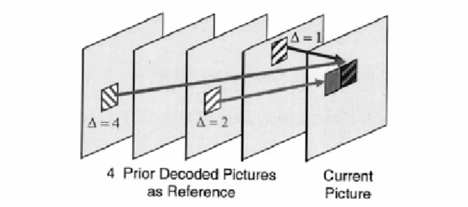
(22) Fig.4. Fractional interpolation for motion compensation. The prediction values for the chroma component are always obtained by bilinear interpolation. Since the chroma components are down-sampled, the motion compensation for chroma has one-eighth sample position accuracy.. The motion vector components are differentially coded using either median or directional prediction from neighboring blocks. Besides, H.264/AVC supports multiple reference frame prediction. That is, more than one prior coded frame can be used as reference for motion compensation as Fig. 5 illustrated.. 10.

(23) Fig. 5. 2.2.3. Multiple reference frame motion compensation. Transform. Similar to previous video coding standards, H.264/AVC utilizes transform coding of the prediction residual. However, the transformation is applied to 4x4 blocks. Instead of a 4x4 discrete cosine transform, an integer transform with similar properties as DCT is adopted. Thus, the inverse-transform mismatches can be avoided due to the exact integer operation of transform. For the 16x16 intra luma or chroma prediction, extra Hadamard transform is applied on the DC coefficients of 4x4 blocks.. There are three reasons for using a smaller size transform. First, the residual signal has less spatial correlation with the advanced prediction. Generally speaking, this transform has less to concern the de-correlation ability. 4x4 transform is essentially as efficient in removing residual correlation as lager transform. Second, the ringing effect is eased for smaller transform. Third, less computation is required in the small size integer transform.. 2.2.4. Quantization. 11.

(24) A quantization parameter is used for determining the quantization of transform coefficients in H.264/AVC. The parameter can take 52 values. The quantized transform coefficients of a block generally are scanned in a zig-zag fashion and transmitted using entropy coding methods. The 2x2 DC coefficients of the chroma component are scanned in the raster-scan order. To simplify the transform, some operation is performed in the quantization stage.. 2.2.5. Entropy coding. In H.264/AVC, there are two methods of entropy coding. The simpler entropy coding method, UVLC, uses exp-Golomb codeword tables for all syntax elements except the quantized transform coefficients. For transmitting the quantized transform coefficients, a more efficient method called Context-Adaptive Variable Length Coding (CAVLC) is employed. In this scheme, VLC tables for various syntax elements are switched depending on already transmitted syntax elements.. In the CAVLC entropy coding method, the number of nonzero quantized coefficients (N) and the actual size and position of the coefficients are coded separately. After zig-zag scanning of transform coefficients, their statistical distribution typically shows large values for the low frequency part and becomes to small values later in the scan for the high-frequency part.. The efficiency of entropy coding can be improved further if the Context-Adaptive Binary Arithmetic Coding (CABAC) is used . In H.264/AVC, the arithmetic coding core engine and its associated probability estimation are specified as multiplication-free low-complexity methods using only shifts and table look-ups. 12.

(25) Compared to CAVLC, CABAC typically provides a reduction in bit rate between 5%–15%. More details on CABAC can be found in [6].. 2.2.6. In-loop deblocking filter. One particular characteristic of block-based coding is the accidental production of visible block structures. Block edges are typically reconstructed with less accuracy than interior. To ease the blocking artifacts due to both prediction and transform operation, an adaptive deblocking filter which can improve the resulting video quality is performed in the motion compensation loop as an in-loop filter. The filter reduces the bit rate typically.. 2.3 Profiles. A profile defines a set of coding tools or algorithms that can be used in generating a conforming bit stream. In H.264/AVC, there are three profiles, which are the Baseline, Main, and Extended Profile. The Baseline profile supports all features in H.264/AVC except the following two feature sets:. ‧ Set 1: B slices, weighted prediction, CABAC, field coding, and picture or macroblock adaptive switching between frame and field coding. ‧ Set 2: SP/SI slices, and slice data partitioning.. The first set of additional features is supported by the Main profile. However, the Main profile does not support the FMO, ASO, and redundant features which are supported by the Baseline profile. The Extended Profile supports all features of the 13.

(26) baseline profile and main profile except CABAC. Baseline profile is used for lower-cost application with less computation resources such as videoconferencing, internet multimedia and mobile application. Main profile supports the mainstream consumer for applications of broadcast system and storage devices. The extended profile is intended as the streaming video profile with extra coding tools for data loss robustness and server stream switching. Fig.6 shows the relationship of these three profiles.. Fig.6 Profiles. 14.

(27) Chapter 3. DATA. MAPPING. AWARE. FRAME. MEMORY. CONTROLLER. 3.1 Backgrounds. Fig.7 Simplified architecture of typical 4-bank SDRAM. 3.1.1 Features of SDRAM. A brief illustration of 4-bank SDRAM architecture is shown in Fig.7. These 15.

(28) kinds of SDRAMs are three-dimensional structures of bank, row, and column. Each bank contains its own row decoder, column decoder, and sense amplifier, while four banks share the same command, address and data buses. SDRAMs provide programmable Burst-Length, CAS Latency, and burst type. The mode register is used to define these operation modes. While updating the register, all banks must be idle, and the controller should wait the specified time before initiating the subsequent operation. Violating either of these requirements will result in unspecified operation.. Fig.8(a) Typical read access in SDRAM. 16.

(29) Fig.8(b) Typical write access in SDRAM. Fig.8(a) and Fig.8(b) shows a typical read and write access. A memory access operation consists of three steps. First, an active command should be sent to open a row in a particular bank, which will copy the row data into the sense amplifier. Second, a read or write command is issued to initiate a burst read/write access to the active row. The starting column and bank address are provided by address bus, and the burst length and type are as defined in mode register in advance. Data for any read/write burst may be truncated with subsequent read/write command as shown in Fig.9(a), and the first data element from the new burst follows either the last element of a completed burst or the last desired data element of a longer burst which is being truncated. Finally, a precharge command is used to deactivate the open row in a particular bank or the open rows in all banks. The bank(s) will be available for a subsequent memory access time after the sense amplifier is precharged. Many SDRAMs provide auto precharge which performs individual-bank precharge function without command issued right after the completion of read/write access. This is 17.

(30) accomplished by setting an index when the read/write access command is sent. Thus we can issue another permitted command during the cycle of precharge command to improve the utilization of command bus.. Fig.9(a) Random read access. Fig.9(b) Random write access. Since each bank can operate independently, a row-activation command can be overlapped to reduce the number of cycles for the row-activation as shown in Fig.10.. 18.

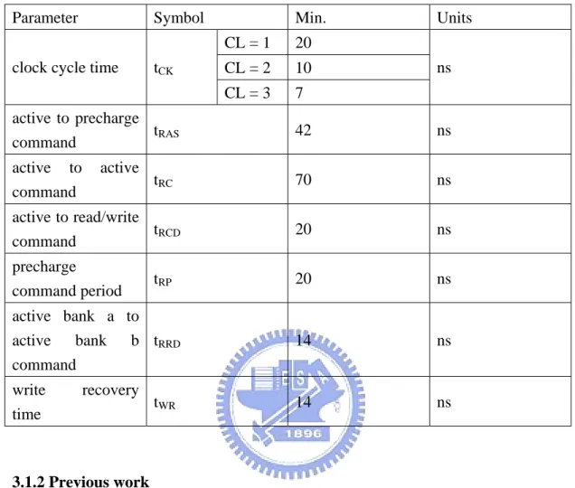
(31) Take a read access as an example. Assume to read 8 data from the SDRAM, and that 4 data lie in row 0 of bank 0 and others lie in row1 of bank 1. Without bank alternating, we need 16 cycles to get 8 data from the SDRAM. This access occupies command bus for 16 cycles. However, only 12 cycles are needed with alternating access and the command bus is busy for 8 cycles. We can send subsequent command to pipeline the following operation. The more data is required, the more cycles can be saved. For 8 data, we gain 25% of speedup for the read memory access latency.. Fig.10 Bank alternating read access. Some important timing characteristics are listed below. The behavior model used in our design is Micron’s MT48LC8M32B2P 256 Mb SDRAM [7] with 4 banks by 4,096 rows by 512 columns by 32 bits.. 19.

(32) Table 1 SDRAM timing characteristics. Parameter. Symbol. clock cycle time. tCK. Min. CL = 1. 20. CL = 2. 10. CL = 3. 7. Units ns. active to precharge tRAS command. 42. ns. active to command. 70. ns. active to read/write tRCD command. 20. ns. precharge command period. 20. ns. active bank a to active bank b tRRD command. 14. ns. write time. 14. ns. active. recovery. tRC. tRP. tWR. 3.1.2 Previous work. Targeted to video codec applications, many papers have been proposed to improve SDRAM bandwidth utilization and achieve efficient memory access. Li [8] develops a bus arbitration algorithm optimized with different processing unit to meet the real-time performance. Ling’s Table 9 controller schedules DRAM accesses in pre-determined order to lower the peak bus bandwidth. Kim’s [10] memory interface adopts an array-translation technique to reduce power consumption and increase memory bandwidth. Park’s [11] history-based memory controller reduces page break to achieve energy and memory latency reduction. For H.264 application, Kang’s [12] AHB based scalable bus architecture and 20.

(33) dual memory controller supports 1080 HD under 130MHz. Zhu’s [13] SDRAM controller employs the main idea of Kim’s memory interface to HDTV application. It focuses on data arrangement and memory mapping to reduce page active overheads so that it not only improve throughput but also provides lower power consumption. However, it doesn’t take the memory operation scheduling into consideration. With careful scheduling, some loss of bus bandwidth introduced by page active operation can be reduced. We combine the data mapping and operation scheduling in our design to decrease the bandwidth requirement for real-time decoding.. 3.1.3 Problem definition. For a memory access, for each time we activate a closed row, we will suffer the latency introduced by SDRAM inherent structure. For read access, the read latency consists of tRP (precharge), tRCD(active) and CAS latency. For write access, the write latency includes tRP (precharge) and tRCD(active). There are two methods to ease this overhead. One is to reduce the required active command. This means either the demand data should lie in as less rows as possible within a single request or the probability of row miss must be as small as possible between successive requests. Since the numbers of row opening is decreased, the latency we suffered can be shortened. Fig.11 shows the effect of row opening reduction on access latency. The other is to apply bank alternating to hide the latency. However, the number of total required operation remains the same. Taking the advantage of banks architecture, the free bank can continue another operation while other banks process requested works, and thus the latency of current access will be overlapped as shown in Fig.12. For such case, the required data should lie in different banks when row miss is happened, or the bank interleaving technique will fail to improve the data bus utilization. 21.

(34) Fig.11 Memory access under different row miss count. Fig.12 Cycles overlapped by bank interleaving technique. For video applications, the memory request is usually to get a determined size of rectangle image from frame memory like those in motion compensation, intra prediction and deblocking filter process. These data are continuous in spatial domain separately and the area we may request between two consecutive blocks has high probability to be overlapped. For instance, when we process motion compensation, the range of data we may need is bounded by block size and search range set during encoding. If the search range is L and the block length is N, a 2L by 2L+N rectangle is overlapped. Data in this region has high probability to be opened in previous block access. Thus we can find a method to avoid the row miss. Fig.13 illustrates an. 22.

(35) example to explain this characteristic.. Fig.13 Possible required area between adjacent blocks. According to the characteristics of video data, the translation between physical location in memory and pixel coordinates in spatial domain will affect the probability of row miss. We can analyze the statistics of video sequence to find an optimized translation to minimize the times of row opening and then the controller can schedule memory operations to enhance the efficiency. As a result, the bandwidth utilization of the same SDRAM can be increased.. 3.1.4 Estimation of bandwidth requirement. H.264 has high efficiency of video compression comparing with previous video processing standards such as MPEG-2 and MPEG-4. This is contributed to its 23.

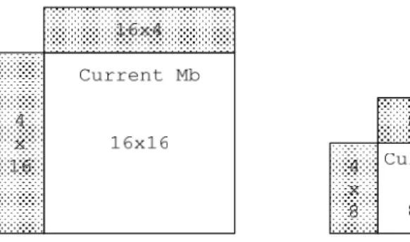
(36) advanced features like fractional pixel interpolation, variable block sizes, multiple reference frames, etc. However, these lead to high bandwidth requirement in implementation. Below we briefly discuss the requirement of bandwidth in different processing unit. Assume that the frame width is W, height is H, the frame rate is F and all are in 4:2:0 format.. Reference frame storage. In H.264 decoder, the processed frame must be store in memory for following. frame. reference.. The. required. bandwidth. is. BWRFS = W * H * (1Y + 0.25Cb + 0.25Cr ) * F. Loop filter. A deblocking filter is adopted in H.264 to improve the subjective quality. For luma, a 16x4 block and a 4x16 block adjacent to current macroblock are referenced while deblocking current macroblock. For chroma, we need to reference an 8x4 block and a 4x8 block. As a result, the bandwidth we required is BWLP = (W / 16) * ( H / 16) * ((16 * 4 * 2)Y + (8 * 4 * 2) Cb + (8 * 4 * 2) Cr ) * F Fig.14. illustrate the reference blocks for loop filter.. 24.

(37) Fig.14 Reference blocks for deblocking fliter. Motion compensation. H.264 supports variable block size motion compensation to enhance coding efficiency as shown in Fig.15.. Fig.15 Block types in H.264. Beside, sub-pixel interpolation is applied to further improve the performance but extra bandwidth is required to meet the real-time decoding. Table 2 lists the maximum reference block size for different block type. Considering the worst case, all blocks are broken into smallest 4x4 size with maximum reference blocks and all frames are p-frame except first frame. The requirement of bandwidth is 25.

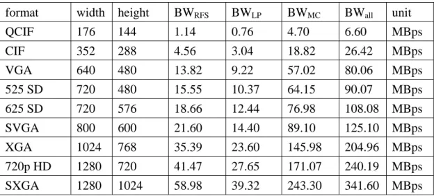
(38) BWMC = (W / 16) * ( H / 16) * ((9 * 9 * 16)Y + (3 * 3 * 16) Cb + (3 * 3 * 16) Cr ) * F. The effect of first frame is neglected in above formula.. Table 2 Maximum area of reference blocks. luma block. max. size of chroma block reference block. max. size of reference block. 16 x 16. 21 x 21. 8x8. 9x9. 16 x 8. 21 x 13. 8x4. 9x5. 8 x 16. 13 x 21. 4x8. 5x9. 8x8. 13 x 13. 4x4. 5x5. 8x4. 13 x 9. 4x2. 5x3. 4x8. 9 x 13. 2x4. 3x5. 4x4. 9x9. 2x2. 3x3. Summing up all above three cases, we can get rough bandwidth requirement for H.264 decoder. The bandwidth for different frame size is listed in Table 3 with assuming that frame rate is 30 fps in all cases.. Table 3 Rough estimation of required bandwidth in different frame size. format. width. height. BWRFS. BWLP. BWMC. BWall. unit. QCIF. 176. 144. 1.14. 0.76. 4.70. 6.60. MBps. CIF. 352. 288. 4.56. 3.04. 18.82. 26.42. MBps. VGA. 640. 480. 13.82. 9.22. 57.02. 80.06. MBps. 525 SD. 720. 480. 15.55. 10.37. 64.15. 90.07. MBps. 625 SD. 720. 576. 18.66. 12.44. 76.98. 108.08. MBps. SVGA. 800. 600. 21.60. 14.40. 89.10. 125.10. MBps. XGA. 1024. 768. 35.39. 23.60. 145.98. 204.96. MBps. 720p HD. 1280. 720. 41.47. 27.65. 171.07. 240.19. MBps. SXGA. 1280. 1024. 58.98. 39.32. 243.30. 341.60. MBps. 26.

(39) 1080 HD. 1920. 1080. 93.31. 62.21. 384.91. 540.40. MBps. With the growth of frame size, the required bandwidth increase rapidly and motion compensation processing unit dominates the demand for memory bandwidth. However, SDRAM bandwidth can not achieve 100% utilization. It needs to improve the performance with optimized data arrangement and careful operation scheduling.. 3.2 optimization of memory access. 3.2.1 Intra-request optimization. In this section we discuss the memory access operation within a single request and build a mathematic model to describe this behavior. According to the model, we can find optimized mapping between physical location and the position in spatial domain. With the optimized translation, the probability of row miss can be reduced. The maximum of row break times is 3. Employing the bank interleaving mechanism, some latency can be hidden to further improve the bus utilization.. In H.264 decoder, the most bandwidth consuming part is motion compensation. In which, luma interpolation takes most of bandwidth for motion compensation. With the data arrangement optimization based on luma interpolation behavior, we can improve the common case of bandwidth usage. For luma interpolation, the referenced data ranges from 21x21 to 4x4 rectangles. These data can be characterized with starting point, data width, and data height.. 27.

(40) Fig.16 1-D row break probability model. To ease analysis without loss of generality, we degrade this 2-D problem to 1-D domain. Assume that a SDRAM row contains L pixels and N continuous data are requested. The situation of row miss could be as follows. For the case without row misses, the starting point shall lie in the first L-N position of the row. However, if the starting points lie in last N-1 pixels, row miss happened. The last N-1 positions build an alert interval as shown in Fig.16. Assuming the probability of starting point position is uniform distributed, the probability of row miss is prow−miss −1D =. N −1 L. For constant data length N, larger size of row means fewer row miss and the longer data length leads to higher row-miss probability with fixed row size. Extending above conclusion to 2-D domain, the total row miss consists of horizontal row miss and vertical row miss. The probability of total row miss is prow−miss −2 D =. N X − 1 NY − 1 + LX LY. LX, LY denote the length of memory window in horizontal and vertical separately. However, the row size is fixed for SDRAM. The width and height of the row window are influenced each other. The row miss probability should be adjusted as follows:. 28.

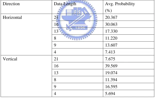
(41) N X − 1 N Y − 1 Ω * ( N X − 1) + L X * ( N Y − 1) , NX, NY, LX >0 + = LX Ω / LX LX * Ω 2. prow−miss −2 D =. where Ω denotes the row size. For worst case, NX = NY = maximum data length. Thus, the row-miss probability has the minimum value when LX is equal to Ω .. In H.264 the data length we may request for motion compensation is 4, 8, 9, 13, 16 and 21 pixels. The length selection is judged by block modes and sub-pixel motion vectors. The distribution of data length is as shown below.. Table 4 Data length distribution. Direction. Data Length. Avg. Probability (%). Horizontal. 21. 20.367. 16. 30.063. 13. 17.330. 8. 11.220. 9. 13.607. 4. 7.413. 21. 7.675. 16. 39.569. 13. 19.074. 8. 11.394. 9. 16.595. 4. 5.694. Vertical. With the increasing of quantization parameter, the encoder tends to choose larger size block mode. This means that the long length data is requested more frequently. The test sequences are crew, night, sailormen, and harbour with 525 SD frame size and QP=32. 29.

(42) However, the starting point doesn’t distribute uniformly in many video sequences. The position number that is divisible by 4, which means the 0th, 4th, 8th, 12th …4kth …pixels of row window in vertical or in horizontal, has higher probability to appear. Generally speaking, p4k is 1.5 to 2.5 times larger than others, where p4k denotes the probability of 0th, 4th, 8th, 12th …4kth …positions. This is because the smallest block length is 4 and the zero motion vector effect. The blocks with zero motion vectors are usually referenced for background image. For larger quantization parameter, this effect becomes more significant. Thus, the row miss probability of H.264 motion compensation is. prow−miss−MC = =. ∑. N X =4 ,8, 9 ,13,16 , 21. LX. ( pN X *. ∑ pn ) +. n = LX − N X +1. ∑. NY = 4 ,8, 9 ,13,16 , 21. LY. ( p NY *. ∑p. m m = LY − NY +1. 5 * PN X 4 + 11 * PN X 9 + 10 * PN X 8 + 16 * PN X 13 + 20 * PN X 16 + 25 * PN X 21 LX + LX / 4. ). +. 5 * PNY 4 + 11 * PNY 9 + 10 * PNY 8 + 16 * PNY 13 + 20 * PNY 16 + 25 * PNY 21 LY + LY / 4 Ω * (a ) + LX * (b) = 5 ΩL X 4 2. Where (a) and (b) are. 5 * PN X 4 + 11 * PN X 9 + 10 * PN X 8 + 16 * PN X 13 + 20 * PN X 16 + 25 * PN X 21......(a ) 5 * PNY 4 + 11 * PNY 9 + 10 * PNY 8 + 16 * PNY 13 + 20 * PNY 16 + 25 * PNY 21.........(b). The PNX4 is the probability of data length equal to 4 pixels in horizontal and we assume p4k is twice than others for simplification.. Applying the statistics in table.4, we can find the row miss probability function is. 30.

(43) 16.866 * Ω + 16.133 * L X Lx * Ω. 2. For Lx >0, this function has a minimum vale when LX equal to 1.04Ω . Typically, a row of a SDRAM can store 16384, 8192 or 4096 bits, that is 2048, 1024 or 512 pixels. The SDRAM behavior model we used contains 2048 pixels in a row. The optimized window size should be a 46x44 rectangle.. However, it is hard to implement the translation with the 46x44 windows. We adjust the window size to 64x32. Because 32 and 64 are powers of 2, the translation can be easily implemented with bits shift. Fig.17 shows the statistics of row miss in different window size. The test sequences are crew, night, sailormen, and harbour in 525 SD frame size.. Comparing with the linear translation like 1x2048 and 2048x1 window, the 64x32 mapping reduces about 84% in miss rate. The rows with large size can decrease the probability of row break, thus the 32x32 window has higher row miss count than 64x32. Due to the video sequences characteristic, the occurrence of horizontal break is more frequent than vertical. The widow with slightly large width can lead to better performance.. 31.

(44) row miss prob. in different windows 70. miss rate (%). 60 50. 2048x1 64x32 46x44 32x64 32x32 1x2048. 40 30 20 10 0 2048x1 64x32 46x44 32x64 32x32 1x2048. qp20. qp32. qp40. 44.83032999 6.820379894 6.778230921 6.846469165 7.403632408 44.8864127. 47.24833619 7.529893801 7.545193255 7.60661285 8.116680411 49.0488445. 54.99977362 9.3924985 9.533249351 9.521609834 9.96107406 58.74551384. Fig.17 Miss rate in different row windows. Fig.18 Translation of physical location and image position. Fig.18 illustrates the mapping between physical location in memory and image position in spatial domain. The latency of single request can be reduced with bank alternating operation. Considering the SDRAM architecture, the banks we requested 32.

(45) in single request should be different. It is because this will lead to the more reduction of latency. Thus, it is easy to find a good bank arrangement that all adjacent banks are different as shown in Fig.19. If the requested data amount is less than twice of DRAM window size for both vertical and horizontal directions, the maximum of row break occurrence is 4. For example, for a 64x32 window, the request data length shall smaller than 128x64.. Fig.19 Bank arrangement with optimization. 3.2.2 The memory operations in single request. With the data arrangement mentioned before, the requests can be classified to 3 kinds as shown in Fig.20. We open all required rows at the beginning of every request. Thus we can reduce the control overhead and ease the hardware design.. Case 1: all data of single access are contained in a row.. It is clear that this case introduces no row miss, since all the data to be requested 33.

(46) are stored in a row. The memory operation contains the row activation, data reading and precharging. Fig.21 shows the operations under case 1. L+4 cycles are needed to complete this access, where L denotes the number of accessed data.. Case 2: all data of single access are contained in two rows. The data may be discontinuous in horizontal or in vertical as illustrated in Fig.20.. In this case, we suffer two row miss since the accessed data are contained in different rows. However, they are in different banks. We can shorten the latency with bank alternating access. Fig.21 shows the operations of case 2. We open the rows we may access, read the data in determined order and then precharge the opened row. Total cycle count is L+5.. Fig.20 Request classification. Case 3: all data of single access are stored in four rows. The data break in horizontal and vertical as illustrated in Fig.20.. Four row breaks are encountered in this case. Due to the limitation of tRRP, one cycle latency is introduced to meet timing requirement. Fig.21 illustrates the 34.

(47) operations. The number of total cycles is L+7.. Fig.21 Request operations in different cases. bank cross distribution 100% 90% 80% 70% 60% case 3 case 2 case 1. 50% 40% 30% 20% 10% 0% case 3 case 2 case 1. qp20. qp32. qp40. 1.763961321 23.55624675 74.67979193. 1.536542139 20.01307293 78.45038493. 1.088995216 14.54669593 84.36430885. Fig.22 Distribution of request kinds. The distribution of the cases mentioned before is as shown above. The test sequences are crew, night, sailormen, and harbour in 525 SD frame size. With the increasing of quantization parameter, the bank-across cases decreases rapidly. Encoder tends to choose zero motion vector in high QP, and thus the data for motion 35.

(48) compensation process usually lie in the same row within single request. According to the statistics, case 1 takes most cases in total accesses. This means we usually only need to open one row in single request. Since our data arrangement reduces the row miss times, the bandwidth can be enhanced comparing with the other mappings.. 3.2.3 Burst length selection. The SDRAMs support burst read access to enhance the bus utilization. However, this feature introduces extra overhead in the data arrangement discussed above. We put all data required in single request in one row as possible as we can. But the locations within a request are usually discontinuous. Every time we encounter the data discontinuity, we may waste cycles to read the unnecessary data. Take 9 by 9 block for example, we waste 9 cycles with BL = 2, 9 cycles with BL = 4 and 45 cycles with BL = 8 as shown in Fig.23. Many motion compensation units prefer received data in z scan order to ease data reuse. This characteristic worsens the over access problem.. 36.

(49) Fig.23 Wasted data in different data burst length. Though the read burst can be truncated by another read or burst terminate command, extra control overhead increase the complexity of hardware design. Thus we set BL equal to 1 in our design. For every required data, we take one cycle to set the address of read/write access. All data we access are necessary for video process.. 3.2.4 Inter-request optimization. In intra-request optimization, we have determined the optimized data mapping to reduce the row misses. Furthermore, for successive requests, the requested data has high probability to be stored in the same row due to overlapped search range. This 37.

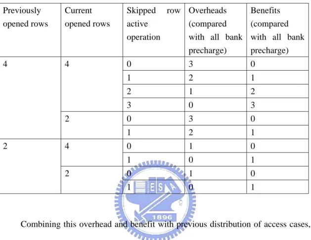
(50) access can get the same benefit as the intra request without any row miss. However, there is still a certain amount of data that is stored in different rows, and thus closing unused rows by precharging the banks and opening the new rows will cause row miss. To reduce such row misses, we shall consider when and how to close the row by precharing.. The SDRAMs support auto precharge which performs the same individual-bank precharge function right after the last read/write command without requiring an explicit command. When we get data in z scan order, the data location may cross banks frequently. We may read one data from row 0, then from row 1 and then from row 0 again. With auto precharge, an extra row break is introduced. Thus mutual precharge operation leads to high bandwidth efficiency. When we finish a request, we should check whether the opened rows still active in next request or not. If the rows has been opened in the previous request, we can skip the row active and precharging operation. In our design, since we open all required rows at beginning of the request, we suffer no latency with the row-cross data access.. There are two types of precharge command, precharge all banks or precharge single bank. Precharing each bank separately is preferred to easy reduce row miss. If not all rows are the same with previous request, we can also skip the row active operations that have been done before. However, individual precharging has overheads to send more explicit commands to close corresponding rows while only one command is needed for all banks precharging. The benefit we gain from 2 row breaks to 1 break is comparatively small with the one from no break to 1 break. The overheads and benefits in different situation are as listed below.. 38.

(51) Table 5 Overheads and benefits of separate bank precharging comparing with all banks precharging. All numbers are in cycles.. Previously opened rows. Current opened rows. Skipped row Overheads active (compared operation with all bank precharge). Benefits (compared with all bank precharge). 4. 4. 0. 3. 0. 1. 2. 1. 2. 1. 2. 3. 0. 3. 0. 3. 0. 1. 2. 1. 0. 1. 0. 1. 0. 1. 0. 1. 0. 1. 0. 1. 2 2. 4 2. Combining this overhead and benefit with previous distribution of access cases, the actual gain by simulation is about 0.1% in total memory access cycles. The benefit is so small that we can neglect it. Considering the hardware control cost and bandwidth performance, we choose all banks precharging as our solution. Every time we request new data, we will check whether all required rows for current block has been opened or not. If all rows have been opened, we will skip the active and precharging operations. In this case, only the CAS latency is suffered. Otherwise, we need to close rows for previous request and active new rows. The suffered latency for this case includes tRP(precharge), tRCD(active) and CAS latency. The average row miss and required cycles with all banks precharging is listed in Table 6.. 39.

(52) Table 6 Average miss rate and required cycles in motion compensation. Test sequences = crew, night, sailormen, and harbour with 525 SD frame size QP. 20. 32. 40. miss rate without 6.82 detection (%). 7.53. 9.39. miss rate with 1.45 detection (%). 1.28. 1.16. enhancement (%). 78.62. 82.48. 86.79. required cycles. 79802862. 75043239. 58408725. 7.50. 5.84. required frequency 7.98 (MHz). Fig.24 shows the memory operations under row miss and row hit detection. With the detection mechanism, we can reduce about 80% of row miss comparing with no detection mapping. To meet the real time luma motion compensation process, the required frequency of SD frame size is about 8MHz.. Fig.24 Memory operation under row miss and row hit. In order to take the advantage of row active operation skipping, we should separate the read and write request in different memories. This is because the location of read and write data lies in different frames. We store reference and current frame data in different rows according to the result of inner request optimization. Thus we 40.

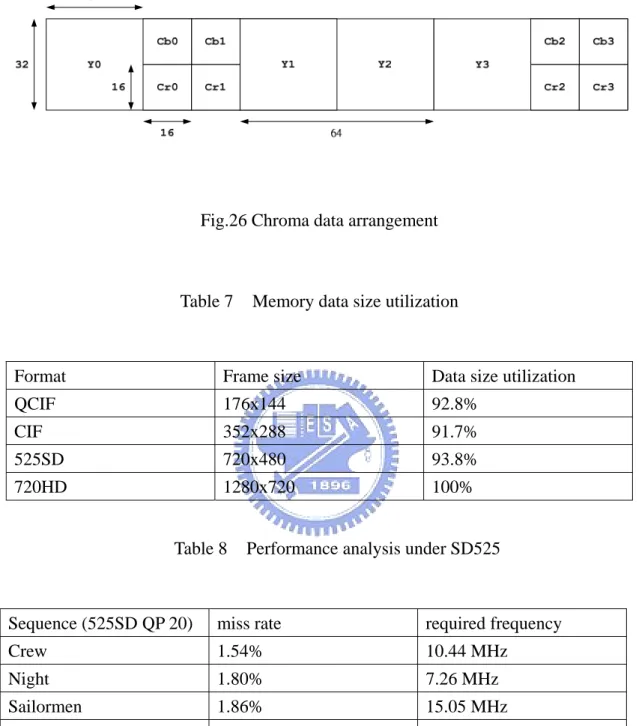
(53) need dual channel environment such as conventional ping-pong structured memories, which one stores reference frame and another stores current frame. Fig.25 shows the read/write operation in I-frame and P-frame. Typically speaking, the write latency is hide by read latency since we do not suffer row cross situation when writing.. Fig.25 Read/write operation in I-frame and P-frame. Considering the interleaved decoding flow of chroma component, the data arrangement should be as shown in Fig.26 to gain the benefit from active operation skipping. Three rows build a set to store four luma 32x32 block data and their corresponding chroma data. However, we suffer the loss of memory data size utilization. For instance, at the tail of every image row, we may only need to store Y2, Cb2 and Cr2, and thus we waste the data size for Y3, Cb3, Cr3. With this data arrangement, the single request of chroma interpolation may access different row data in the same bank, which is guaranteed not to be happened in luma interpolation by the bank arrangement. This may cause more latency. However, since the block size and reference data access of chroma are relatively small than the ones of luma, the overall performance does not drop too much. Table 7 lists the data size utilization in different format and Table 8 lists the required frequency to support motion compensation of 41.

(54) luma and chroma component in 525 SD format.. Fig.26 Chroma data arrangement. Table 7. Memory data size utilization. Format. Frame size. Data size utilization. QCIF. 176x144. 92.8%. CIF. 352x288. 91.7%. 525SD. 720x480. 93.8%. 720HD. 1280x720. 100%. Table 8. Performance analysis under SD525. Sequence (525SD QP 20). miss rate. required frequency. Crew. 1.54%. 10.44 MHz. Night. 1.80%. 7.26 MHz. Sailormen. 1.86%. 15.05 MHz. Harbour. 1.93%. 14.20 MHz. Average. 1.78%. 11.74 MHz. 3.2.5 Overall access flow. The flows of data read and write is as shown in Fig.27. For read access, we check if all required rows are opened in previous request at begging. If yes, we go 42.

(55) throw to data access stage. If not, we should close all used rows and determine how many rows should be active in current request. There are three cases that we need to open one, two or four rows. For the case that we open four rows, read commands can be inserted between 2nd, 3rd and 4th active commands with bank alternating access. After the row open operation, we can random access data in demand order. When we finish the final data access, the flow goes back to the initial state and preparing the operations in following requests. For read chroma data, if we suffer bank conflict which means we access different row data in the same bank during single request, we spilt them in two separate requests at the beginning. For write access, since the data within single macroblack never cross different rows and typically the elementary storage unit is one macroblock, only one row could be opened in single request. The row number checking can be simplified.. 43.

(56) Fig.27 Read and write request process flow. 3.2.6 Performance in different frame size. The bandwidth performance differs in different frame size due to the sequence characteristics and encoding of mode selection and motion vectors. With larger frame size, the row miss rate slightly increases. This is due to few rows contained in one small frame. For instance, four rows cover 32% area of the qcif format frame. Thus, most of the reference data are stored in the opened rows. However, if we don’t apply. 44.

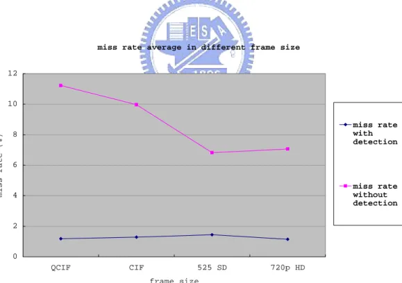
(57) detection mechanism, the miss rate varies largely and becomes irregular in small frame sizes. The result differs dramatically depending on the sequences contents. This is due to that reference data concentrate in some regions especially in small sizes. When these regions cross rows, the probability of row breaks increase greatly. For large frame size, the effort becomes light due to the more uniform distribution of reference data. Below illustrates the miss rate in different frame sizes. With the detection, the row break probability remains almost the same in different frame size. For large size, the increase of bandwidth is mainly to support the growth of decoding data throughput instead of the row setup overheads. The test sequences are akiyo, mobile, stefan, coastguard and foreman in QCIF and CIF, crew, night, sailormen, and harbour in 525SD and parkrun, shield and stockhelm in 720HD with QP = 20.. miss rate average in different frame size 12. miss rate (%). 10 miss rate with detection. 8. 6 miss rate without detection. 4. 2. 0 QCIF. CIF. 525 SD. 720p HD. frame size. Fig. 28 Miss rate average in different frame sizes. 45.

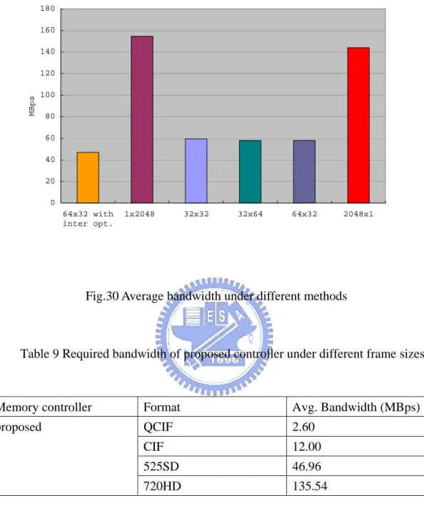
(58) miss rate variance in different frame size 30. miss rate variance. 25. without detection. 20. 15. with detection. 10. 5. 0 QCIF. CIF. 525 SD. 720p HD. frame size. Fig.29 Miss rate variance in different frame sizes. 3.2.7 Performance comparison. Fig.30 illustrates the average required bandwidth for motion compensation of luma and chroma components. With the 64x32 window mapping, the required bandwidth reduces about 97MBps comparing to 1x2048 mapping. With the inter request optimization described in 2.2.4, we can further reduce about 10MBps. As a result, the required bandwidth is 46.96MBps, where the test sequences are crew, night, sailormen, and harbour in 525 SD frame size with QP = 20.. 46.

(59) Average Bandwidth 180 160 140. MBps. 120 100 80 60 40 20 0 64x32 with inter opt.. 1x2048. 32x32. 32x64. 64x32. 2048x1. Fig.30 Average bandwidth under different methods. Table 9 Required bandwidth of proposed controller under different frame sizes. Memory controller. Format. Avg. Bandwidth (MBps). proposed. QCIF. 2.60. CIF. 12.00. 525SD. 46.96. 720HD. 135.54. Table. 9. lists. the. average. required. ban. dwidth of the proposed controller under different frame sizes ranged from QCIF to 720 HD. Comparing with the proposed controller, Zhu [13] only choose a 64x64 window mapping and does not take more detailed mode selection of memory operation into consideration. For example, auto precharge is still used in Zhu’s design.. 47.

(60) When data cross different rows, the extra latency introduced by the auto precharge command can not be reduced. Besides, the inter-request optimization described in previous section 3.2.4 can not be applied if we select auto precharge as our precharging method. Wang [14] schedules the memory operation and arranges the data organization to ease the access latency. However, Wang’s bank arrangement may cause different row data accesses in the same bank during single interpolation request, which only happens in chroma interpolation of proposed controller. Wang does not find an optimized data mapping for the intra-request access as discussed in section 3.2.1. When decoding large frame size, this case may occur more frequently, and thus the performance may decrease. On the other hand, Wang’s bank arrangement tends to open multiple banks within a single request, while most cases only need to open one banks in the proposed as shown in Fig.22. The proposed controller may be more suitable for the applications with low power issues.. Besides, take the memory access of displayer into consideration, the required bandwidth is as listed in Table 10. The bandwidth contains the access cycles of frame data and latency caused by row break. According to our data arrangement, every 64 columns a row break will happen for every row in the frame. Since the displayer refreshment is row by row in spatial domain, this kind of breaks can not be hidden by bank alternating operation. For every row break in memory access, 4 cycles are required to meet the SDRAM timing constraint, where 2 cycles are for active command and the others are for precharge command. However, the insertion of displayer refreshment accesses may introduce extra latency because they break statistics of motion compensation accesses which proposed controller is optimized with. For the worst case, inter-request optimization can not help to reduce latency and every time the switch of memory access causes a row break which will introduce 48.

(61) another 4 cycles latency. In our assumption, at the end of every image row in displayer refreshment process, the switch of motion compensation requests and displayer refreshment ones will happen. For the best situation, the required bandwidth is only the summation of two kinds of accesses due to the assumption that no extra latency is introduced by the insertion of displayer refreshment. If we use the same memory for both displayer refreshment and motion compensation, the actual bandwidth should lie between the worst case and the best one as listed in Table 10.. Table 10 BW requirement with displayer refresh issue. Sequence format. BW for displayer BW in best case BW in worst case (MBps). (MBps). (MBps). QCIF. 1.16. 3.76. 4.75. CIF. 4.64. 16.64. 20.21. 525SD. 16.81. 63.83. 74.77. 720HD. 42.12. 187.66. 109.98. 3.3 Hardware architecture of memory controller. The entire memory controller is shown in Fig.31. The controller includes a read address generator, read command generator, write address generator, write command generator, arbitrator, data masker, detection unit and control unit.. 49.

(62) Fig.31 Memory controller design. The read address generator is mainly composed by two 11-bit adders and temp registers. One adder calculates the address of horizontal coordinate, and the other is for vertical. The translation between image coordinate and memory address is as shown in Fig.32. In horizontal calculation, the last 6 bits present column address, the 6th bit means the bank address and the first 4 bits are for representation of row address. While vertical calculating, the first 5 bits are translated to row address, the 5th bit is for bank selection, the 2nd to 4th bits are decoded as column address and the last 2 bit determine the byte index which controls the data masker for final output. Frame index. 50.

(63) is sent from outer component and it contains the information of frame indexes. The bit arrangement can support up to 2048 by 2048 frame size. For larger sizes, the row address part should be adjusted. Every time a new request is sent to this controller, the address generator calculates the end address at the beginning. According to these address, we can check whether all required rows are opened or not. Besides the detection, we can determine how many rows should be opened by the bank address. If the bank addresses of stating point and ending point are different, we suffer one row break in the corresponding axis. If we suffer row breaks in both direction, four bank alternating access is necessary for this request. After the detection and operation selection, the address generator is used to generate the address of read data. The temp registers store the turning points which will be used to calculate following addresses. The increments are decoded from the data length from outer signal and operation states from control unit.. Fig.32 Bit arrangement in address generator. The detection unit detects the row activation requirement and sends to control unit to determine the operation modes. The read command generator receives the modes operations and translates them to memory commands. The data masker buffers. 51.

(64) two words and mask out the redundant data with the masking logic. The output data is organized as that the first n bits are affective if not all output is demand. The masking information comes from control unit and the byte index of address generator. The data masker also sends data enabling signal to connected processing unit. The write address generator and write command generator are duplicates of the ones of read. The arbiter allocates read/write data and command to and from the external memories.. The control unit includes total control FSM and motion compensation scheduler FSM. The total control FSM schedules the memory operation like active, read/write and precharge. To determine the operations, the necessary information like that all rows has been opened or not and how many row should be opened is supported by the detection unit. Once the total control FSM changes to read/write mode, the controller is controlled by motion compensation scheduler FSM. It controls address generator to produce demand column address. The address order is aimed to generate the z scan order for motion compensation. If we want other orders, we add another read/write scheduler. Fig.33 illustrates the z scan order when motion compensation.. Fig.33 Scan order for 4x4 luma blocks Through this memory controller, the optimization of data arrangement and the 52.

(65) row prediction can be realized with simple hardware design. The separation of horizontal and vertical address calculation can ease the complexity for cross bank and discontinuous address generation. Comparing with [], this architecture is more friendly for H.264 application due to the z scan order, more flexible block types and sub-pixel interpolation. This controller can effectively enhance the bus utilization meanwhile the throughput of video decoder can be improved.. 3.4 Summary. In this chapter we proposed a SDRAM memory controller dedicated for H.264 video decoder. We analyze statistics of video sequences and characteristics of SDRAMs. According to the information, we set an optimized data arrangement which can effectively reduce the memory setup overheads. Besides, we employ a simple prediction mechanism to enhance the performance. We schedule the memory access with the bank alternating technique and have a chance to skip the row active operations. The memory controller is helpful to improve the bus utilization and ease the bandwidth requirement in overall decoder. The performance of controller doesn’t crashes in large frame size. The row miss remains stable in different frame size and sequences. By the way, this controller performance can be enhanced with advanced DRAM like DDR and wider data bus width.. 53.

(66) Chapter 4. ENTROPY DECODER. 4.1 UVLC decoder. In H.264/AVC, the Exp-Golomb coding, also known as UVLC, is adopted for all syntax except fixed codes and the quantized transform coefficients. The UVLC entropy coding uses a single finite-extent codeword table. Thus, this coding type is constructed in a regular way, characterized by having predetermined code pattern [15]. Instead of designing a different VLC table for each syntax element, only mapping to the exp-Golomb code table is customized according to the data statistics. These mapping can be divided into four kinds, unsigned element (ue), signed element (se), truncated element (te) and mapped element (me).. Fig.34. Exp-Golomb code construction. Exp-Golomb codes are variable length codes with a regular construction. The code structure is separated by the bit string into “prefix” and “suffix” bits as shown in Fig.34. The leading N zeros and the middle “1” can be regarded as “prefix” bits. The 54.