在PMC模式下對k元n維立方體局部診斷能力之研究

國

立

交

通

大

學

資訊科學與工程研究所

碩

碩

碩

碩

士

士

士

士

論

論

論

論

文

文

文

文

在 P M C 模 式 下 對 k 元 n 維 立 方 體

局

部

診

斷

能

力

之

研

究

Local Diagnosability of k-ary n-cube Networks

under the PMC Model

研 究 生：林銘皇

在 PMC 模式下對 k 元 n 維立方體局部診斷能力之研究

Local Diagnosability of k-ary n-cube Networks under the PMC Model

研 究 生：林銘皇 Student：Ming-Huang Lin

指導教授：譚建民 Advisor：Jimmy J.M. Tan

國 立 交 通 大 學

資 訊 科 學 與 工 程 研 究 所

碩 士 論 文

Submitted to Institute of Computer Science and Engineering College of Computer Science

National Chiao Tung University in partial Fulfillment of the Requirements

for the Degree of Master

in

Computer Science

June 2006

Hsinchu, Taiwan, Republic of China

在

在

在

在 PMC

PMC 模式下對

PMC

PMC

模式下對

模式下對 k

模式下對

kk

k 元

元 n

元

元

nn

n 維立方體

維立方體

維立方體

維立方體

局部診斷能力之研究

局部診斷能力之研究

_{局部診斷能力之研究}

局部診斷能力之研究

研 究 生：林銘皇 指導教授：譚建民 教授

國 立 交 通 大 學 資 訊 科 學 與 工 程 研 究 所

摘要

摘要

摘要

摘要

在這篇論文裡，我們介紹了一個新的衡量錯誤診斷能力的方法，稱為局部診

斷能力。依據不同的觀點，來做不同的詮釋研究，從原本廣域的觀點轉換成局

部的觀點來觀察。在新的觀點下，我們展示了一個簡單的方法來診斷一個多處

理機系統。我們把局部診斷能力的研究應用在連線無損壞的 k 元 n 維立方體上，

並觀察得每個點的價數(degree)即為其局部診斷能力。接著我們把局部診斷能

力的研究應用在有任意連線損壞的 k 元 n 維立方體上。根據我們在這篇論文裡

的証明，在任意的損壞連線數不超過 2n−2 個數時，每點的局部診斷能力仍為每

點的價數。此外，我們提出了一個更為有效率的演算法來診斷錯誤的發生。

關鍵字：診斷能力，局部診斷能力，k 元 n 維立方體，價數。

Local Diagnosability of k

Local Diagnosability of k

Local Diagnosability of k

Local Diagnosability of k-

--

-ary n

ary n

ary n-

ary n

--

-cube

cube

cube

cube

Networks under the PMC Model

Networks under the PMC Model

Networks under the PMC Model

Networks under the PMC Model

Student：Ming-Huang Lin

Advisor：Jimmy J.M. Tan

Institute of Computer Science and Engineering

National Chiao Tung University

Abstract

In this thesis, we introduce a new measure for diagnosability, called local

diagnosability, by changing the original global viewpoint to a local viewpoint. With this

new viewpoint, we yield an easy way to diagnose a multiprocessor system. We apply the

concept of local diagnosability to k-ary n-cube with no missing links and the local

diagnosability of each node is exactly the degree of each node. Then we investigate the

local diagnosability of k-ary n-cube with arbitrarily distributed missing links. Based on

the result proved in this thesis, the number of missing links can be up to 2n−2 and the

local diagnosability of each node is the remaining degree of each node. Moreover, we

propose a more efficient diagnosis algorithm.

Contents

1 Introduction 4

2 Preliminaries 6

2.1 Terminology and Preliminaries . . . 6 2.2 Basic properties of Qk n . . . 7 2.3 The PMC Model . . . 8 3 Locally t-diagnosable 12 3.1 Local Diagnosability . . . 12 3.2 Local Diagnosability of Qk

n with No Faulty Edges . . . 14

3.3 Local Diagnosability of Qk

n with Faulty Edges . . . 18

3.4 Diagnosis Algorithm (Counting Algorithm) . . . 25

List of Figures

2.1 Examples of k-ary n-cubes; (a) Q4

1 and (b) Q 3

2. . . 8

2.2 An example of a k-ary n-cubes; (c) Q3 3 . . . 9

2.3 Qk n is divided into Q[0], Q[1], ..., Q[k − 1]. . . 10

2.4 Illustrations of a distinguishable pair (F1, F2). . . 11

3.1 Illustrations of a local distinguishable pair (F1, F2). . . 13

3.2 An illustration of a Type I. . . 15

3.3 An indistinguishable pair of S1, S2 in Q41, but also in Q 2 2. . . 15

3.4 A Type I in Qk 1, for all k ≥ 5. . . 16

3.5 Illustrations of three cases (of the proof of Lemma 6). (a) Case 1, (b) Case 2, and (c) Case 3. . . 17

3.6 An illustration of the proof of Theorem 4. . . 19

3.7 An illustration of indistinguishable pair S1 and S2 (of Qk_n with 2n broken edges). . . 20

3.8 Illustrations of indistinguishable pair S1 and S2 (of Q32 with two broken

edges). . . 21 3.9 Illustrations of case 1 (of the proof of Lemma 7), (a) Case 1.1 and (b) Case

1.2 . . . 22 3.10 Illustrations of case 2 (of the proof of Lemma 7), (a) Case 2.1 and (b) Case

2.2 . . . 28 3.11 Illustrations of case 3 (of the proof of Lemma 7), (a) Case 3.1 and (b) Case

3.2 . . . 29 3.12 Illustrations of case 1 (of the proof of Theorem 5), (a) Case 1.1 and (b)

Case 1.2 (c) Case 1.3. . . 30 3.13 Illustrations of case 2 (of the proof of Theorem 5), (a) Case 2.1 and (b)

Case 2.2. . . 31 3.14 Illustrations of (a) Local syndrome and (b)From left to right, there are

Chapter 1

Introduction

As the rapid development of digital technology, the architecture of multiprocessor system has become more and more complex today, and often with a large number of processors (nodes). It is important to maintain the reliability of such system. Therefore, fault diagnosis has become an important issue in the design of multiprocessor systems.

It is impractical to test each processor (node) individually in a large multiprocessor system, when there are faulty processors (nodes). Preparata et al. [1] first introduced a fault diagnosis model (called PMC model) for system level diagnosis. This is much more efficient than testing one node by one node. Also several different models have been proposed in the literature [2], [3].

Hakimi and Amin [4] proved that a multiprocessor system is diagnosable if it is t-connected with at least 2t + 1 nodes. Besides, a necessary and sufficient condition was given for verifying if a system is t-diagnosable under the PMC model.

In this thesis, we adopt PMC model as the fault diagnosis model and proposed a new measure of diagnosability, called local diagnosability. Besides we investigate the

local diagnosability of k-ary n-cube [5] with no missing links and learn that the local diagnosability of each node is exactly the degree of each node, and the local diagnosability of k-ary n-cube with arbitrarily distributed missing links, as the number of missing links is not exceed 2n − 2, the local diagnosability of each node is the remaining degree of each node.

The rest of this thesis can be categorized as follows: Section 2 provides terminology and preliminaries. Section 3 introduces the concept of local diagnosability and defines the local t-diagnosability of a system. We then study the local diagnosability of k-ary n-cube (Qk

n) in Section 4. Moreover, we propose a fault diagnosis algorithm in Section 5. Finally,

Chapter 2

Preliminaries

2.1

Terminology and Preliminaries

The architecture of an interconnection network can be represented as a graph in which the nodes correspond to processors and the edges to communication links.

Let G = (V, E) be a graph if V is a finite set and E is a subset of {(u, v) | (u, v) is an unordered pair of V }. We say that V is the vertex set and E is the edge set. Two vertices u and v are adjacent if (u, v) is an edge of G. The neighborhood of u, denote by N(u), is {v | (u, v) ∈ E}. The degree deg(u) of a vertex u of G is the number of edges incident with u. The components of a graph G are its maximal connected subgraphs. A component is trivial if it has no edges; otherwise, it is nontrivial. The set of nodes in component C is denoted by Vc and Cx is the component which contains node x. For a set

F ⊂ E, the notation G − F represents the graph obtained by removing the edges F from G.

There are many mutually conflicting requirements in designing the topology for com-puter networks. The n-cube is one of the most popular topologies [6], and the class of k-ary

n-cubes is another commonly used interconnection topology for parallel and distributed systems. In this thesis, we study the local diagnosability of k-ary n-cube.

2.2

Basic properties of Q

The k-ary n-cube Qk

n is a 2n regular graph consists of N = kn nodes, and is highly

symmetric. Each node has the form X = xn−1, xn−2, ..., x0, where 0 ≤ xi ≤ k − 1, for

all 0 ≤ i ≤ n − 1. Two nodes X = x_n−1, x_n−2, ..., x0 and Y = y_n−1, y_n−2, ..., y0 are

interconnected if and only if there exists an i, 0 ≤ i ≤ n − 1, such that xi = yi± 1 (mod

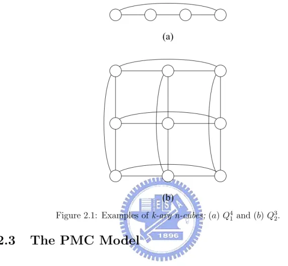
k) and xj = yj, for i 6= j. Figure 2.1. and Figure 2.2. shows some examples of the k-ary

n-cubes.

A k-ary n-cube Qk

n can be decomposed into k copies of Qkn−1 or in general kβ copies

of Qk

n−β subcubes for all β ≤ n. If we refer to d∗(x, y) ∈ E(Q k

n) where x differs from y

in the dth position of bitwise representation, for 0 ≤ d ≤ n − 1, we then have an edge of dimension d. We say that Qk

nis divided into k copies of subgraph, Qkn[0], Qkn[1], ..., Qkn[k−1]

(abbreviated as Q[0], Q[1], ..., Q[k − 1], if there are no ambiguities), along dimension d for some 0 ≤ d ≤ n − 1, and the edges loop around these subgraphs above is the so called, dimension edges. The bitwise represent of Qk

n[l] is labeled by xn−1...xd+1lxd−1...x0, for

every 0 ≤ l ≤ k − 1 (see Figure 2.3). It is clear that each Qk

n[l] is isomorphic to Qkn−1 for

0 ≤ l ≤ k − 1. As a result, there are n ways that a Qk

n can be divided into k copies of

Qk

Figure 2.1: Examples of k-ary n-cubes; (a) Q4

1 and (b) Q 3 2.

2.3

The PMC Model

In the study of multiprocessor systems, there are several different models of self-diagnosis, the PMC Model [1] was adopted each vertex (node) will test all its neighboring vertices (neighboring nodes) and it is assumed that there is no vertex tested by itself.

Definition 1 Under the PMC model, a syndrome σ for system G is defined as follows: for any two distinct adjacent vertices u and v,

σ(u, v) =  



0, if v is tested by u, that u is fault-free and v is fault-free. 1, if v is tested by u, that u is fault-free and v is faulty. 0/1, if v is tested by u, that u is faulty.

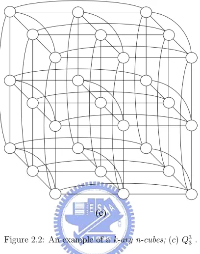
Figure 2.2: An example of a k-ary n-cubes; (c) Q3 3 .

Let σ(F ) represent the set of all syndromes which could be produced if F is the set of faulty vertices.

Definition 2 Two distinct sets F1, F2 ⊂ V are said to be indistinguishable if σ(F1)T σ(F2) 6=

∅ ; otherwise, F1, F2 are said to be distinguishable. We say (F1, F2) is an indistinguishable

pair if σ(F1)T σ(F2) 6= ∅, else, (F1, F2) is a distinguishable pair.

Definition 3 [1] A system of n units is t-diagnosable if all faulty units can be identified without replacement, provided that the number of faults presented does not exceed t.

Q [0] Q [1] Q [k-2] Q [k-1]

Figure 2.3: Qk

n is divided into Q[0], Q[1], ..., Q[k − 1].

Let F1, F2 ⊂ V be two distinct sets and let the symmetric difference F1△F2 = (F1 −

F2)S(F2− F1). |F1| represent the number of nodes in F1.

Lemma 1 [7] A system G(V, E) is t-diagnosable under PMC model if and only if for each pair F1, F2 ⊂ V with |F1|, |F2| ≤ t and F1 6= F2, there is at least one test from

V − (F1S F2) to F1△F2.

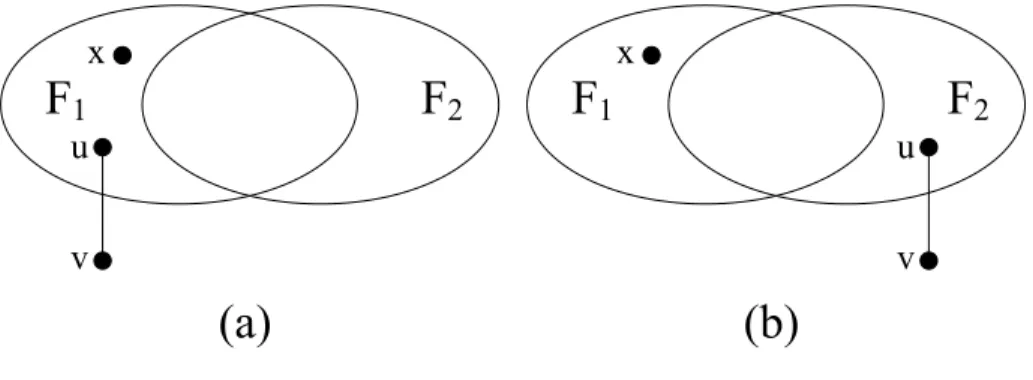
Lemma 2 [9] For any two distinct sets F1, F2 ⊂ V , (F1, F2) is a distinguishable pair if

and only if there exists a vertex u ∈ V − (F1S F2) and there exists a vertex v ∈ F1△F2

such that (u, v) ∈ E (see Figure 2.4).

Theorem 1 [9] Let G(V, E) be the graph of a system G. Then, G is t-diagnosable if and only if, for each vertex set S ⊂ V with |S| = p, 0 ≤ p ≤ t − 1, every component C of G − S satisfies |VC| ≥ 2(t − p) + 1.

1 2 u v 1 2 u v

Chapter 3

Locally t-diagnosable

3.1

Local Diagnosability

Definition 4 A system of n units is locally t-diagnosable at vertex x, F is the set of all faulty units, x can be identified without replacement, provided that the number of faults presented does not exceed t.

Lemma 3 A system G(V, E) is locally t-diagnosable at vertex x under PMC model if and only if for each pair F1, F2 ⊂ V with |F1|, |F2| ≤ t and F1 6= F2, and x ∈ F1△F2, there

is at least one test from V − (F1S F2) to F1△F2.

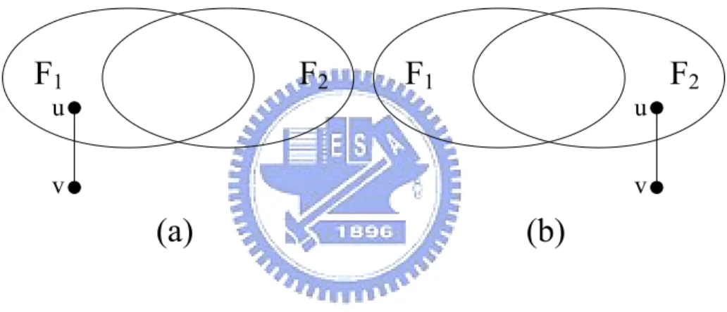
Lemma 4 For any two distinct sets F1, F2 ⊂ V , (F1, F2) is a local distinguishable pair

if and only if there exists a vertex u ∈ V − (F1S F2), a vertex v ∈ F1△F2 and a vertex

x ∈ F1△F2 such that (u, v) ∈ E (see Figure 3.1).

Theorem 2 Let G(V, E) be the graph of a system G. Then, G is locally t-diagnosable at vertex x if and only if, for each vertex set S ⊂ V with |S| = p, 0 ≤ p ≤ t − 1, every component Cx of G − S satisfies |VCx| ≥ 2(t − p) + 1.

1 2 u v 1 2 u v x x

Figure 3.1: Illustrations of a local distinguishable pair (F1, F2).

Proof. We prove |VCx| ≥ 2(t − p) + 1 is necessary by contradiction. Suppose that

there exists a set of vertices S ⊂ V with |S| = p, 0 ≤ p ≤ t − 1 and x 6∈ S such that, in graph G-S, the connected component which x belongs to has strictly less than 2(t − p) + 1 vertices. Let Cx be such a component with |VCx| ≤ 2(t − p). We then arbitrarily partition

VCx into two disjoint subsets, VCx = A1S A2 with |A1| ≤ t − p and |A2| ≤ t − p. Let

F1 = A1S S and F2 = A2S S. Then |F1| ≤ t and |F2| ≤ t. It is clear that there is no

edge between V − (F1S F2) and F1△F2. By Lemma 4, F1 and F2 are indistinguishable

and x ∈ F1△F2. This contradicts to the assumption that G is locally t-diagnosable at

vertex x.

To prove the sufficiency, suppose on the contrary, that G is not locally t-diagnosable at vertex x, i.e., there exists an indistinguishable pair (F1, F2) with |Fi| ≤ t, i = 1, 2

and x ∈ F1△F2. By Lemma 4, there is no edge between V − (F1S F2) and F1△F2. Let

|F1△F2| ≤ 2(t − p), where |S| = p and 0 ≤ p ≤ t − 1. Therefore, there is at least one

component Cx of G − S with |VCx| ≤ 2(t − p), which is a contradiction. This completes

the proof of the theorem.

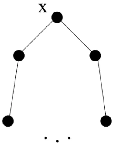
A Type I graph at vertex x is defined by every neighboring node of x must has a different good neighbor to other neighboring nodes of x, (see Figure 3.2).

Theorem 3 Let G(V, E) be the graph of a system G. Then, G is locally t-diagnosable at vertex x, if there exists a Type I subgraph.

Proof. In highly structure, the total number of nodes is 2t + 1, t is the degree of node x (deg(x) = t), and |VCx| ≥ 2t + 1. Each time we remove one node (not include node x) in

the highly structure, the number of nodes will loss connection to x is at most two. So, if we removed a set of nodes P , P ⊂ V with |P | = p, for 0 ≤ p ≤ t − 1, then the number of nodes it will loss is at most 2p. The number of nodes of VCx is the total number of nodes

2t + 1 minus the number of losing nodes 2p. As a result represent, |VCx| ≥ 2(t − p) + 1.

By Theorem 2, G at node x is locally t-diagnosable.

3.2

Local Diagnosability of Q

with No Faulty Edges

In the following, if we not mention that a k-ary n-cube is missing links or with faulty edges, then we consider k-ary n-cube as a complete k-ary n-cube. On the other hand, we do not discuss the case of missing nodes.

We study case by case on the growth of the size to show that whether k-ary n-cue is locally t-diagnosable or not. It is clear that Q4

1 and Q 2

2 (usually we take Q 2

Figure 3.2: An illustration of a Type I.

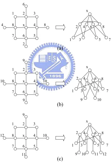
of n = 2) is not locally 2-diagnosable, because of there exists an indistinguishable pair S1 ∈ {x, a} and S2 ∈ {y, b} at node x by Lemma 4 (see Figure 3.3).

1 2

Figure 3.3: An indistinguishable pair of S1, S2 in Q41, but also in Q 2 2.

Lemma 5 There exists a Type I at any vertex x ∈ Qk

1, and for all k ≥ 5.

Proof. With out loss of generality, let x be any node in Qk

1 for all k ≥ 5 and the degree

of each node x is 2. Therefore, every neighboring node of x (N(x)) has a link to test another node which has not been tested yet, for all k is greater than 5. Clearly, there exists a Type I in any node x (see Figure 3.4).

Figure 3.4: A Type I in Qk

1, for all k ≥ 5.

Lemma 6 There exists a Type I at any vertex x ∈ Qk

2, and for all k ≥ 3.

Proof. Since k-ary n-cube is highly symmetric. With out loss of generality, let node x be any node in the Qk

2. Then, we have three different cases: 1) k = 3, 2) k = 4, and 3)

k > 4.

Case 1: k = 3.

Because there are four different nodes which are adjacent to the neighboring nodes of x, by Pigeonhole Principle, each node of the N(x) has at least a link to test a different node.

Case 2: k = 4.

Because there are six different nodes which are adjacent to the neighboring nodes of x, by Pigeonhole Principle, each node of the N(x) has at least a link to test a different node.

Case 3: k > 4.

Because there are eight different nodes which are adjacent to the neighboring nodes of x, by Pigeonhole Principle, each node of the N(x) has at least two links to test two different nodes. (See Figure 3.5) 1 2 3 8 x 4 7 6 5 8 4 6 2 x 2 4 6 8 1 3 5 7 1 2 3 8 x 4 7 6 5 10 10 9 9 x 2 4 6 8 1 3 5 7 10 9 1 2 3 8 x 4 7 6 5 10 12 9 11 x 2 4 6 8 1 3 5 7 10 9 11 12

Figure 3.5: Illustrations of three cases (of the proof of Lemma 6). (a) Case 1, (b) Case 2, and (c) Case 3.

For all the cases prove above, we observe that there exists a Type I at any vertex x ∈ Qk

2, for all k ≥ 3.

Theorem 4 There exists a Type I at any vertex x ∈ Qk

n, for some n ≥ 2 and for all

k ≥ 3.

Proof. We prove this theorem by induction on n. Clearly by Lemma 6, this theorem is true for Qk

2, for all k ≥ 3. Assume it holds for some n ≥ 2, for all k ≥ 3. We now show

that it holds for n + 1. Let Qk

n+1 be obtained from k copies of subgraph Qkn, denoted by Qkn[0], Qkn[1], ..., and

Qk

n[k − 1], by adding dimension edges between them.

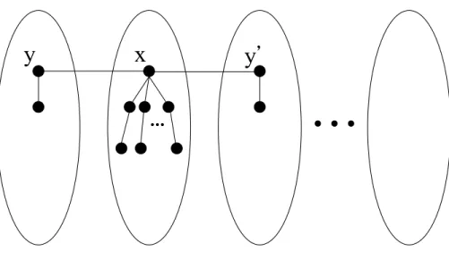
Without loss of generality, we take node x to be one node of the subgraph Qk

n. Let y

and y′ _{be the neighboring nodes of x exclusive those in the subgraph Q}k

n which contains

the node x. For the degree of each node is two, therefore there are one more node (not the node x) links to y and y′_{, y and y}′ _{are in different subgraph. Also, by induction}

hypothesis, there exists a Type I at node x ∈ Qk

n (see Figure 3.6).

Consequently, this theorem holds.

3.3

Local Diagnosability of Q

with Faulty Edges

Commonly, there are faults occur in a multi-processor system. In this thesis, we discuss the issue when the linking edges are broken or missing, called faulty edges.

But exactly, how many missing links or broken edges will make the system not locally t-diagnosable for any vertex x? Let t be the degree of each node, that is 2n. When there

’

Figure 3.6: An illustration of the proof of Theorem 4.

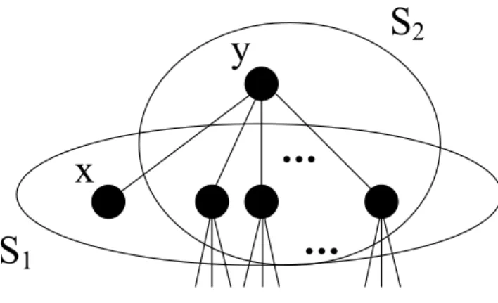
are 2n broken edges then we learn that, if all these 2n broken edges gather at one specific node, then the system is not locally t-diagnosable at this node. Because this node is totally isolated, there are no any edges linking to this node. Further more, if there are 2n − 1 broken edges, simply as above, let all these 2n − 1 broken edges gather at one specific node x, and let node y be the only node connected to x. Then the system is not locally t-diagnosable at node y. By lemma 4, there exists a indistinguishable pair, S1 = N(y) and S2 = yS N(y) − x , |S1| = t and S2 = t (see Figure 3.7). As results show

above, we then investigate when there are 2n − 2 broken edges. Q3

2 with two broken edges is not locally t-diagnosable at vertex x, x ∈ Q 3

2 , because

of there exists an indistinguishable pair S1 ∈ {x, a, b, c} and S2 ∈ {y, a, b, c}, by lemma 4

1

2

Figure 3.7: An illustration of indistinguishable pair S1 and S2 (of Qk_n with 2n broken

edges).

Lemma 7 Let Qk

2, for all k ≥ 4, has no more than two faulty edges. Then there exists a

Type I at any vertex x ∈ Qk

2, for all k ≥ 4.

Proof. Let node x be any node in Qk

2, we discuss the number faulty edges around node

x. We have three cases: 1) There are two faulty edges on the neighboring edges of x, 2) There is exactly one faulty edge on the neighboring edges of x, and 3) No faulty edges are the neighboring edges of x.

Case 1: There are two faulty edges on the neighboring edges of x.

Case one can be further discussed into two subcases, for how many faulty edges are there on the dimension edges.

Case 1.1: In case one, there are two faulty edges on the dimension edges. Case 1.2: In case one, there are only one faulty edge on the dimension edges. (see Figure 3.9).

Figure 3.8: Illustrations of indistinguishable pair S1 and S2(of Q32 with two broken edges).

Clearly, we learn that each neighboring node of x in the Case 1.1 and Case 1.2, connects at leat two different nodes which are not including node x.

Case 2: There is exactly one faulty edge on the neighboring edges of x. Case two can be further discussed into two cases, with k = 4 and k > 4. Case 2.1: k = 4.

Because there are six different nodes which are adjacent to the neighboring nodes of x, and there are only one more faulty edge may happened, by Pigeonhole Principle, each node of the N(x) has at least two links to test two different nodes.

Figure 3.9: Illustrations of case 1 (of the proof of Lemma 7), (a) Case 1.1 and (b) Case 1.2 .

Case 2.2: k > 4.

Because there are seven different nodes which are adjacent to the neighboring nodes of x, and there are only one more faulty edge may happened, by Pigeonhole Principle, each node of the N(x) has at least two links to test two different nodes.

(see Figure 3.10).

Case 3: No faulty edges are the neighboring edges of x.

Case 3.1: k = 4.

Because there are six different nodes which are adjacent to the neighboring nodes of x, and there are two faulty edges may happened, by Pigeonhole Principle, each node of the N(x) has at least one link to test a different nodes.

Case 3.2: k > 4.

Because there are seven different nodes which are adjacent to the neighboring nodes of x, and there are two faulty edges may happened, by Pigeonhole Principle, each node of the N(x) has at least one link to test a different nodes.

(see Figure 3.11).

For all the cases prove above, we observe that there exists a Type I at any vertex x ∈ Qk

2, with no more than two faulty edges, for all k ≥ 4.

Theorem 5 Let |F | be the number of faulty edges in Qk

n, for some n ≥ 2 and for all

k ≥ 4. Then there exists a Type I in any vertex x ∈ Qk

n, for some n ≥ 2, for all k ≥ 4

and |F | ≤ 2n − 2.

Proof. We prove this theorem by induction on n. Clearly by Lemma 7, this theorem is true for Qk

2, for all k ≥ 4. Assume it holds for some n ≥ 2, for all k ≥ 4. We now show

that it holds for n + 1. Let Qk

n+1 be obtained from k copies of subgraph Qkn, denoted by Qkn[0], Qkn[1], ..., and

Qk

n[k − 1], by adding dimension edges between them. Let x be any node in Qkn+1. We

investigate two cases: 1) There are not more than two faulty edges and at least one faulty edges on the dimension edges along some dimension, 2)There are not more than one faulty

edges on the dimension edges.

Case 1: There are not more than two faulty edges and at least one faulty edges on the dimension edges along some dimension.

We discuss the case, when n + 2 ≤ |F | ≤ 2n. By Pigeonhole Principle, there are at least two faulty edges on the dimension edges along some dimension d, 0 ≤ d ≤ n.

Thus there are at most two dimensional edges that connect to each node, we then have three more subcases:

Case 1.1: There are two faulty edges on the dimension edges and this two faulty edges are adjacent to the node x.

By induction hypotheses, there exists a Type I at node x.

Case 1.2: There are one faulty edge on the dimension edges and the faulty edge is adjacent to the node x.

Let y be the neighboring node of x, because each node has at least two good neighbors and by induction hypotheses, there exists a Type I at node x.

Case 1.3: There are no faulty edges on the dimension edges which is adjacent to the node x.

Let y and y′ _{be the neighboring nodes of x, because each node has at least two good}

neighbor and by induction hypotheses, there exists a Type I at node x. (see Figure 3.12).

We discuss the case, when 1 ≤ |F | ≤ n + 1. There are not more than one faulty edge on the dimension edges and there are at most n + 1 faulty edges along dimension n + 1. For each subgraph there are at most n broken edges, we have 2n − 2 ≥ n, for some n ≥ 2. There are at most two dimension edges that connect to each node. We have two more subcases:

Case 2.1: There are one faulty edge on the dimension edges, and the faulty edge is connected to the node x.

Let y be the neighboring node of x, because each node has at least two good neighbor and by induction hypotheses, there exists a Type I at node x.

Case 2.2: There are no faulty edges on the dimension edges which is connected to the node x.

Let y and y′ _{be the neighboring node of x, Similarly above, each node has at least two}

good neighbor and by induction hypotheses, there exists a Type I at node x. (see Figure 3.13).

3.4

Diagnosis Algorithm (Counting Algorithm)

Base on Type I, we propose an algorithm to diagnose a system and the time-complexity is O(n log n). It is more efficient than the fault identification algorithm which the time-complexity is O(n2.5_{) [7].}

Let node p be the node which adjacent to node x, and node q be the node which adjacent to node p, both p and q are in the Type I of node x. A vote is said to be

positive, negative or spoilt is defined as follows: Positive vote, if σ(q, p) = 0 and σ(p, x) = 0. Negative vote, if σ(q, p) = 0 and σ(p, x) = 1.

Spoilt vote, if σ(q, p) = 1 and σ(p, x) = 0, or σ(q, p) = 1 and σ(p, x) = 1

A local syndrome is the set of syndrome which are tested in Type I of node x, showed as above.

(see Figure 3.14).

In a locally t-diagnosable system, the number of faulty nodes are under t. First, we have a set of local syndrome from the Type I of node x, then we count the positive votes and negative votes to tell if node x is faulty or fault free. Third, provided that the positive votes are greater than or equal to the negative votes, we say the node x is fault free, vice versa.

Theorem 6 For the local syndrome from Type I of node x of a locally t-diagnosable system, the node x is fault-free if the positive votes are greater than or equal to the negative votes.

Proof. By contradiction, let node x be the faulty node. Without loss of generality, we have A positive votes, B negative votes and C spoilt votes in the set of local syndrome of node x, for A + B + C = t and deg(x) = t. As the node x is faulty, the minimum number of faulty nodes of Type I is 2A + C + 1, for a positive vote have two faulty nodes, a spoilt vote have at least one faulty node and the node x is one faulty node.

the total faulty nodes are greater than or equal to t + 1. This contradicts the assumption that the node x is fault-free.

Theorem 7 For the local syndrome from Type I of node x of a locally t-diagnosable system, the node x is faulty if the positive votes are less than the negative votes.

Proof. By contradiction, let node x be the faulty-free node. Without loss of generality, we have A positive votes, B negative votes and C spoilt votes in the set of local syndrome of node x, for A + B + C = t and deg(x) = t. The minimum number of faulty nodes of Type I is 2B + C, for a negative vote have two faulty nodes and a spoilt vote have at least one faulty node.

As a result, 2B + C > A + B + C, for A − B < 0. Because A + B + C = t, the total faulty nodes is greater than t. This contradicts the assumption that the node x is faulty.

1 2 3 x 4 7 6 5 9 8 8 x 2 4 6 1 3 5 7 8 9 1 2 3 x 4 7 6 5 9 8 10 x 2 4 6 1 3 5 7 8 9 10

Figure 3.10: Illustrations of case 2 (of the proof of Lemma 7), (a) Case 2.1 and (b) Case 2.2 .

1 2 3 8 x 4 7 6 5 10 10 9 9 x 2 4 6 8 1 3 5 7 10 9 1 2 3 8 x 4 7 6 5 10 12 9 11 x 2 4 6 8 1 3 5 7 10 9 11 12

Figure 3.11: Illustrations of case 3 (of the proof of Lemma 7), (a) Case 3.1 and (b) Case 3.2 .

’

Figure 3.12: Illustrations of case 1 (of the proof of Theorem 5), (a) Case 1.1 and (b) Case 1.2 (c) Case 1.3.

’

Figure 3.13: Illustrations of case 2 (of the proof of Theorem 5), (a) Case 2.1 and (b) Case 2.2.

Figure 3.14: Illustrations of (a) Local syndrome and (b)From left to right, there are positive, negative, spoilt, and spoilt votes.

Chapter 4

Conclusion

In this thesis we introduce a new concept, called local diagnosability, and we studied the local diagnosability of k-ary n-cube both with no missing links and with missing links. We then proved that the local diagnosability of each node of k-ary n-cube equals to the degree of each node of k-ary n-cube, with the missing links limited to the number of 2n − 2. Moreover, by observing whether there exists a Type I at a node of k-ary n-cube, we can determine whether a node of k-ary n-cube is locally t-diagnosable. By the method described in this thesis, we represented an efficient algorithm to diagnose a multiprocessor system.

Bibliography

[1] F. P. Preparata, G. Metze, and R. T. Chien, ”On the Connection Assignment Prob-lem of Diagnosable Systems,” IEEE Trans. Electronic Computers, vol. 16, no. 6, pp. 848–854, Dec. 1967.

[2] J. Maeng and M. Malek, ”A Comparison Connection Assignment for Self-Diagnosis of Multiprocessors Systems,” Proc. 11th Int’l Symp. Fault-Tolerant Computing, pp. 173–175, 1981.

[3] M. Malek, ”A Comparison Connection Assignment for Diagnosis of Multiprocessor Systems,” Proc. Seventh Int’l Symp. Computer Architecture, pp. 31–35, 1980. [4] K. L. Hakimi and A. T. Amin, ”Characterization of Connection Assignment of

Di-agnosable Systems,” IEEE Trans. Computers, vol. 23, no. 1, pp. 86–88, Jan. 1974. [5] L. Gravano, G. Pifarre, P. Berman, and J. Sanz, ”Adaptive Deadlock- and

Livelock-Free Routing with All Minimal Paths in Torus Networks,” IEEE Trans. Parallel and Distributed Systems, vol. 5, no. 12, pp. 1,233–1,251, Dec. 1994.

[6] F.T. Leighton, Introduction to Parallel Algorithms and Architectures: Arrays · Trees · Hypercubes, Morgan Kaufmann, San Mateo, CA 1992.

[7] A. T. Dahbura and G. M. Masson, ”An O(n2.5_{) Fault Identification Algorithm for}

Diagnosable Systems,” IEEE Trans. Computers, vol. 33 no. 6, pp. 486–492, June 1984.

[8] Guey-Yun Chang, Gerard J. Chang, and Gen-Huey Chen, ”Diagnosabilities of Reg-ular Networks,” IEEE Trans. Parallel and Distributed Systems, vol. 16 no. 4, pp. 314–323, Apirl 2005.

[9] Pao-Lien Lai, Jimmy J. M. Tan, Chien-Ping Chang, and Lih-Hsing Hsu, ”Conditional Diagnosability Measures for Large Multiprocessor Systems,” IEEE Trans. Comput-ers, vol. 54 no. 2, pp. 165–174, February 2005.