利用分部合成達到人物動作參數空間擴展與延伸之研究

全文

(1)!. ୮ Ҥ ҫ ೮ δ Ꮱ! !. !. !. !. !. ֍෾ᣯѠ໓ঔ‫!ެے‬ Ⴧ !̀ !ኢ !͛ !. 利用分部合成達到人物動作參數空間擴展與延伸之研究 Parameterized Motion Interpolation and Extrapolation Using Partial Blending. 研究生：陳彥儒指導教授：林奕成. 助理教授. ̚!ර!ϔ!઼!!˝!Ȉ!̱!!ѐ!˛!͡!.

(2) 利用分部合成達到人物動作參數空間擴展與延伸之研究 Parameterized Motion Interpolation and Extrapolation Using Partial Blending. 研究生：陳彥儒. Student：Yan-Ju Chen. 指導教授：林奕成. Advisor：I-Chen Lin. 國立交通大學多媒體工程研究所碩士論文. A Thesis Submitted to Institute of Multimedia Engineering College of Computer Science National Chiao Tung University in partial Fulfillment of the Requirements for the Degree of Master in. Computer Science July 2007 Hsinchu, Taiwan, Republic of China. 中華民國九十六年七月.

(3) 利用分部合成達到人物動作參數空間擴展與延伸之研究. 研究生：陳彥儒. 指導教授：林奕成博士. 國立交通大學多媒體工程研究所. 摘要要獲得準確且真實的人物動作資料，動態動作捕捉是最常使用的技術之一。但是在如遊戲的互動應用上，要如何才能有效的利用並控制這些動作資料仍是令人困擾的問題。在本論文中，我們提出一個在使用不足的動作資料下，擴增角色動作可能性的合成方法。首先我們在時間上對齊這些動作資料樣本，使其呈同步播放的狀態，並將初始動作的朝向都調整成相同以建立參數空間。為了對這些動作資料達到更大化的利用，我們把整個人體之動作分區段。對每個部分分別做合成以及角度上的調整後再接合起來，就可以產生自然且更多樣化的動作。此初始空間在使用我們的動作調整方式後會進一步的擴大。使用者只要指定參數空間的一個位置，就可以得到攻擊到該目標的動作。此方法可以在動作資料有限的情況下應用於武打遊戲中，且可以事先估測可能的攻擊範圍。關鍵字：動態動作捕捉，動作合成，分部混合 I.

(4) Parameterized Motion Interpolation and Extrapolation Using Partial Blending. Student: Yan-Ju Chen. Advisor: Dr. I-Chen Lin. Institute of Multimedia Engineering National Chiao Tung University. ABSTRACT. Human motion capture is one of the most plausible techniques to acquire realistic animation data. However, in interactive applications, e.g. TV games, how to interactively and accurately control the captured data is still a troublesome issue. In this thesis, we present a blending method to extend the possibility of human actions from imperfect motion data. We first align example motions in time and adjust their facing directions to build a initial constraint parameter space. To more efficiently utilize the motion data, we segment human body into several parts. After angular adjustments to each body part individually, more various but natural-looking motion can be synthesized by splicing all the segments back. With our method, the range of the space is extended. Users can simply assign the normalized position in the parameter space, and get a motion that hit the desired target. The proposed method can provide an accurate motion prediction and apply to fighting games with limited motion data. Keyword: motion capture, motion synthesis, partial blending II.

(5) Acknowledgements. First of all, I would like to thank my advisor, Dr. I-Chen Lin, for his help and guidance in the past two years. Also, I thank for all members of Computer Animation and Interactive Graphics Lab. for their assistance and comments. Finally, I am grateful to my family for their support and encouragement.. III.

(6) Contents 摘. 要……………………………………………………………………………………I. ABSTRACT…………………………………………………………………………………..II ACKNOWLEDGEMENTS..………………………………………………………………...III CONTENTS....………………………………………………………………………………IV LIST OF FIGURES………………………………………………..………………………....V LIST OF TABLES…………………………………………………………………………..VII 1. INTRODUCTION…………………………….…………………………………….........1 1.1 Motivation….…………………………………………………………………………1 1.2 Overview………………………………………………………………………….…..3 2. RELATED WORK………………………………………………………………………..6 3. PREPROCESS PHASE………………………………………………………………….11 3.1 Time Alignment………………………………………………………………………11 3.2 Parameter Extraction and Denser Sampling…………………………………………16 4. RUNTIME PHASE………………………………………………………………………19 4.1 Human Body Segmentation………………………………………………………….19 4.2 Parameter Query, Body Part Splicing, and Joint Orientation Adjustments………….20 4.3 Motion Length Rearrangement………………………………………………………29 5. EXPERIMENTAL RESULTS…………………………………………………………...30 5.1 Environment and Sample Data………………………………………………………30 5.2 Results…………………………..……………………………………………………30 5.3 Experimental Evaluation and Analysis………………………………………………35 5.4 Discussion…………………………………………………………………………....40 6. CONCLUSION AND FUTURE WORK……………………………………………...…42 7. REFERENCE…………………………………………………………………………….43. IV.

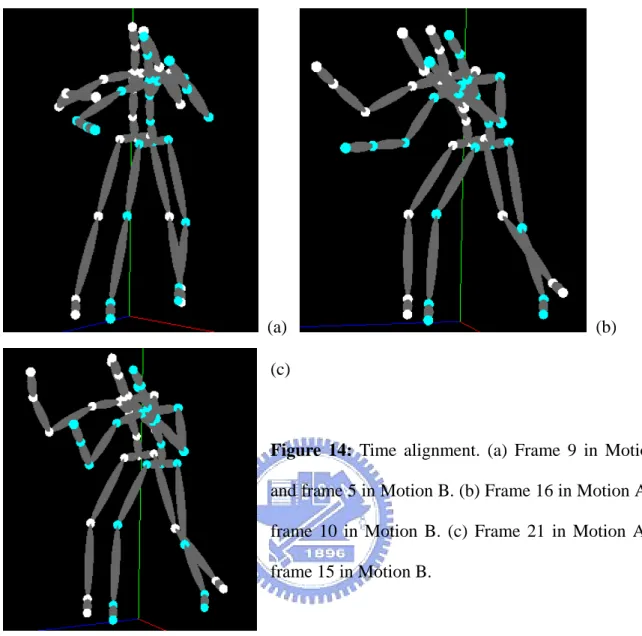
(7) List of Figures Figure 1: Flowchart of the whole framework…………………………………………...…….4 Figure 2: Detailed steps in the preprocess phase.…………………………………...………...5 Figure 3: Detailed steps in the runtime phase.………………………………………………...5 Figure 4: Motion retargeting. (a) Original motion. (b) Retargeting to a smaller-scale skeleton. (c) Retargeting to a longer body with shorter limbs…………………………………………..6 Figure 5: Motion transitions apply to path fitting. The motions are generated to fit a word “motion”……………………………………………………………………………………….7 Figure 6: Time alignment path. Play motions according to the indexes of the alignment path makes these two motions do actions simultaneously……………………………….…………8 Figure 7: (a) Before sampling. There is a significant error between the desired location and the result motion. (b) After denser sampling. More parameters are produced, and more accuracy is provided…………………………………………………………………….…….9 Figure 8: Reliability map. The blue areas represent high reliability, while the red areas represent low reliability……………………………………………………….……………..10 Figure 9: When carrying a heavy box, the green motion leans back to balance the weight of the box………………………………………………………………………………………..10 Figure 10: Calculating frame distance. (a) Two motion frames differ in facing direction and location in the world. (b) Representing two motion frames in terms of joint positions. (c) Apply T transformation on one point cloud for pose matching with the other one………….12 Figure11: A distance grid graph of two motions……………………………………………..13 Figure 12: The path in red shows time alignment between Motion A and Motion B……..…14 Figure 13: Motion A (white joint) and Motion B (blue joint) in original timing. (a) Frame 5. (b) Frame 10. (c) Frame 15.………………………………………………………………….14. V.

(8) Figure 14: Time alignment. (a) Frame 9 in Motion A and frame 5 in Motion B. (b) Frame 16 in Motion A and frame 10 in Motion B. (c) Frame 21 in Motion A and frame 15 in Motion B.………………………………………………………………..……………………………15 Figure 15: Time alignment of a punching motion set. (a) Ready to attack. (b) The attack moment………………………………………………………………………………………16 Figure 16: Denser sampling. Each little red dot represents the motion attack to that position……………………………………………………………………………………….17 Figure 17: The white dots represent the original attack space. We extend the space to the red frame. The motions whose parameters are within the red frame can still be synthesized…...18 Figure 18: The human skeleton hierarchy model……………………………………………20 Figure 19: Joint angular adjustment…………………………………………………………21 Figure 20: Parameter query for motion synthesis……………………………………………22 Figure 21: Hierarchical adjustments of punching motion…………………………………....24 Figure 22: Angular difference of adjustment joints between two motions…………………..25 Figure 23: Comparison between adjust right arm directly and hierarchical adjustment…….26 Figure 24: Unnatural kicking result by using the adjustment scheme of punching motion…27 Figure 25: Right leg orientation adjustment with extra “lift up” or “lay down” for kicking motion………………………………………………………………………………………..28 Figure 26: There is an angular difference in the hip vector of motions that kick differs in height…………………………………………………………………………………………29 Figure 27: An example of time alignment………………………………………………...…29 Figure 28: Straight punch…………………………………………………………………….31 Figure 29: Hook punch……………………………………………………………………....32 Figure 30: Straight kick……………………………………………………………………...33 Figure 31: Side kick………………………………………………………………………….34. VI.

(9) List of Tables Table 1: Statistics of hit position difference………………………………………………….35 Table 2: Hook punch. (a) Regular interpolation with 9 motions. (b) Partial blending with 8 motions……………………………………………………………………………………….36 Table 3: Hook punch. (a) Regular interpolation with 9 motions. (b) Partial blending with 8 motions…………………………………………………………………………………….…37 Table 4: Straight kick. (a) Regular interpolation with 8 motions. (b) Partial blending with 7 motions………………………………………………………………………………….……38 Table 5: Straight kick. (a) Regular interpolation with 8 motions. (b) Partial blending with 7 motions……………………………………………………………………………………….39. VII.

(10) 1. Introduction 1.1 Motivation Character animation has been widely used in real world, especially in games, cartoon, and movie industry. To acquire accurate, realistic, and natural-looking animation data, motion capture is one of the most satisfactory techniques used in recent years. To capture one’s action, a common approach, optic mocap, is to place numbers of sensors on an actor, usually at important joint positions. When the actor performs actions, several calibrated cameras track these sensors to estimate joint positions and orientations. After data cleaning and correction by the artist manually, clean motion data are produced. With motion capture, one may get almost any kind of motion that the actor is able to perform. For instance, it is used to acquire complex martial art motions in most modern fighting games. However, if all of the motion resources are extracted by motion capture, the cost will be expensive, and they require large storage. Furthermore, motion data itself also lack flexibility. So how to enrich the usage of the original captured data becomes a significant issue. And several motion editing approaches has been proposed.. One of the most known approaches to synthesize motions is motion blending. Suppose we have a set of “logically similar” motion data, which means the actor performs the same action. For example, punching motions in the same style but different in attack directions. Once these motions are time-warped together, a new motion can be constructed by a weight combination of the whole data set. After applying a denser sampling, that is, using more pre-designed weight combination sets to blend more motions and extract their parameters, a parameterized motion space can be established. Users may control the parameter in the space freely to produce desired motions.. 1.

(11) Though the method is quite useful, the range of the parameter space is restricted by the quality and quantity of the original motion data. The range of plausible motion we can produce is also limited within the affine summation space. To build a complete shape of parameter space, a well-designed motion capture procedure has to be accomplished, and sufficient motion clips with the same style are also needed. Suppose we want to construct a parameter space for a set of hook-punch motions. The actor’s facing directions have to be the same, and their ready poses have to be as similar as possible. Then, the actor tries to hook-punch toward various direction with the same ready pose in order to enlarge the parameter space. However, the database may not always be “good” enough for us to build desired space. Usually there are defects.. Our goal is to utilize limited motion captured data but create motions that are able to attack a variety of directions and positions. Since we focus on interactive usages, especially in fighting games, the process should be done in real-time. To achieve this purpose, we proposed an example-based method to extend defective parameter space established from imperfect motion data set.. From our observation, we found that a fighting action can be regarded as combination of two behaviors: waist turning from an initial orientation to a proper direction and arm-or-leg attack at a given height. That is, we no longer treat human body as just one single unit. By contrast, we segment a human body into several parts, and apply blending techniques to those parts individually. Given sets of fighting actions, we separate them into different categories according to the body part that performs the attack. So there will be two main types of motions — punching motion and kicking motion. Then, we establish a defective parameter space using these data, and extend it to a possible partial blending space. When a user assigns a desired attack position which is not within the original space, we query two parameters in 2.

(12) the original space. One is used to decide the turning part; the other one is used to decide the attack part. Once we derive the correlations between the two motions, joint orientation adjustments are applied to each body part so as to make the actor hit the desired target as close as possible. The body parts are then spliced together to get the final result — a new motion attacking a position not in the original parameter space. Due to its simple and interactive control, it can be applied to advanced game controls easily. The proposed blending by body parts allows motions to be extrapolated to new expanded region. While the attack region was known in advance, motion prediction is another evident application.. 1.2 Overview When we get a set of sample motions with a similar action but different in direction, and plan to synthesis motions with more various directions, we need to establish an initial parameter space for the full-body sample motions in advance. The parameters are received by interpolation among the sample motions. To get good blending results, we time-align the motions to the same length for action synchronization. The procedure is described in Chapter 3.. After the space is established and extended, a user can assign a position in the extended space to produce a new motion. If it is not in the original space, partial blending is put into practice. Our system will query two parameters in the original space, and apply angular adjustments dependent on the motions they represent. One stands for the orientation movement, the other one is for the attack height. The result motion is then resized in length for proper timing. More detail is described in Chapter 4.. 3.

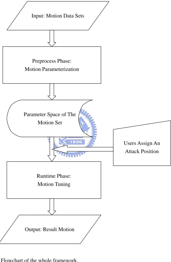
(13) The following graph (Figure 1) shows the whole framework:. Input: Motion Data Sets. Preprocess Phase: Motion Parameterization. Parameter Space of The Motion Set. Users Assign An Attack Position. Runtime Phase: Motion Tuning. Output: Result Motion. Figure 1: Flowchart of the whole framework.. 4.

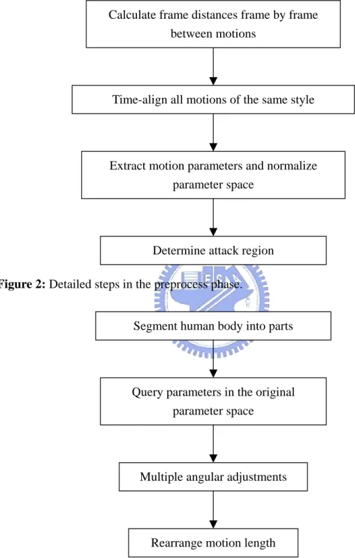
(14) There are further detailed steps in the preprocess phase and the runtime phase. Following are two graphs (Figure 2, Figure 3) that show each step in order: Calculate frame distances frame by frame between motions. Time-align all motions of the same style. Extract motion parameters and normalize parameter space. Determine attack region Figure 2: Detailed steps in the preprocess phase. Segment human body into parts. Query parameters in the original parameter space. Multiple angular adjustments. Rearrange motion length. Figure 3: Detailed steps in the runtime phase.. 5.

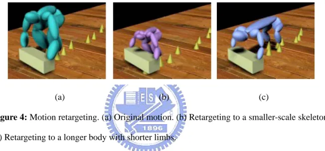
(15) 2. Related Work There are various editing or synthesis schemes to modify captured data for different purposes. Gleicher [6] proposed a method called “retargeting” to map a motion from the original skeleton to another one but keep significant constraints, as shown in Figure 4. For a walking motion, the feet must step right “on” the ground but not penetrate it or float up, and each footstep also needs to locate on the same spot.. (a). (b). (c). Figure 4: Motion retargeting. (a) Original motion. (b) Retargeting to a smaller-scale skeleton. (c) Retargeting to a longer body with shorter limbs.. Another mechanism is called “transition”. This technique smoothly connects the end of one motion clip to the start of another in time domain to generate a longer continuous motion. In practice, transition does not always happen on either side of a motion but may take place on an arbitrary frame in a motion clip. The critical issue is to decide the best transition point which results in a smooth transition. It’s reasonable to assume that the more similar the two frames are, the more seamless transition becomes. Kovar et al. [13] proposed a distance metric to quantify the “similarity” of two poses and using a rigid transformation function to adjust one pose, so it will become the closest match for the target one. Then a graph structure was designed to record the transition nodes and motions that could be smoothly transited. Further application falls on applying transition to a desired purpose like path fitting, 6.

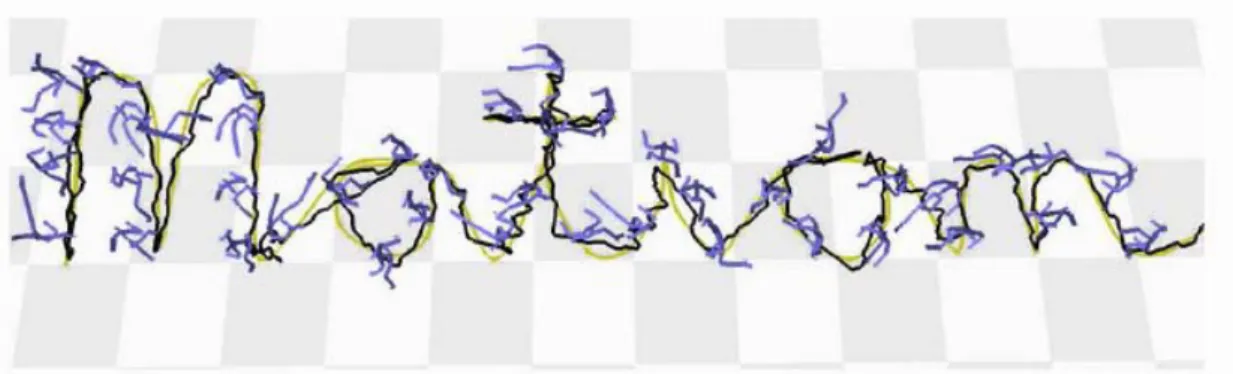
(16) locomoting on a designed path, as shown in Figure 5. Gleicher et al. [7] rearranged the graph structure by collecting similar nodes into a hub node, and varied the possibility of transition. The additional process to accomplish transition could be easily performed by applying transformations among the entrance, exit, and the “common pose”, which is the representative of the hub node.. Figure 5: Motion transitions apply to path fitting. The motions are generated to fit a word “motion”.. To attain a smooth transition, an intuitive interpolation scheme is using a weight set of (0.5, 0.5) on both frames of the two motions at the transition point. Moreover, if we expand this interpolation to a few more frames, and apply a weight function from (1, 0) to (0, 1) gradually, we will get a smoother result. While extending this idea to the whole motion clip, the procedure becomes the foundation of “blending”. The main issue now turns to not only find the most similar poses of two motions but to figure out the total alignment of multiple motion clips.. Kovar and Gleicher [11] employed the distance cost metric proposed earlier on each pair of motions to form a 2D grid graph. This graph shows the similarity relations between all pair of frames of the two motions. Then, they find a minimal-cost connecting path that best aligns these two motions in time domain, as shown in Figure 6. After all paths were. 7.

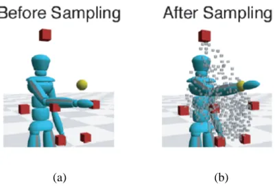
(17) combined together, blending can be applied to make new motions.. Figure 6: Time alignment path. Play motions according to the indexes of the alignment path makes these two motions do actions simultaneously.. They [12] use this idea to classify motions into different categories. Starting with a random sample motion, and apply the method to search other similar motions in the database as the outcome of classification. They also proposed an approach to directly control the blended motions. To achieve this goal, they defined and extracted parameters from a set of motion that best represent the type of those motions. For a punching motion set, the wrist joint might be the defined parameter, and the punching positions were extracted. For a walking cycle motion set, the root joint might be the defined parameter, and the vertical projections of final root positions were extracted. After denser sampling, more parameters will be produced, as shown in Figure 7. Collecting these parameters together forms a discrete parameterized motion space. Users can simply assign a location in the space, and the system will respond a set of blending weights that blend the sample motions most closely to the assigned location.. 8.

(18) (a). (b). Figure 7: (a) Before sampling. There is a significant error between the desired location and the result motion. (b) After denser sampling. More parameters are produced, and more accuracy is provided.. Other research uses various approaches to achieve motion interpolation. Grochow et al. [8] presented an Inverse Kinematics (IK) system and a learning mechanism for motion data training. New motions can be edited by controlling a few constraint parameters. Mukai and Kuriyama [14] proposed a statistical approach to motion prediction and a modified Radial Basis Function (RBF)-like distribution function to construct a smooth parameter surface. And provided a way to estimate the reliability of the predicted motion, as shown in Figure 8. Glardon et al. [5] translated different speeds and types of locomotion data to a new space and applied hierarchical Principal Component Analysis (PCA) for data dimension reduction and style classification. In the hierarchical PC structure, they discovered the relationship between the principal component and its corresponding speed value. Therefore, interpolation as well as little extrapolation of the speed value can be performed on this peculiar space to get new PC coefficient, so as to get the edited motion.. 9.

(19) Figure 8: Reliability map. The blue areas represent high reliability, while the red areas represent low reliability.. The concept of motion editing by segmenting human body into parts and combining different parts from different motions was used by Heck et al. [9]. They treat human motion as a combination of upper-body action and lower-body locomotion. So the body is divided into two parts. They time-align the two target motions, and compute a rotation transformation for the splice point to keep natural balance. For a walking motion, when left arm swings forward, right leg should also be in front of the main body. In Figure 9, when a person carries a heavy box using both hands, the upper-body should leans back to balance the weight of the box.. Figure 9: When carrying a heavy box, the green motion leans back to balance the weight of the box. 10.

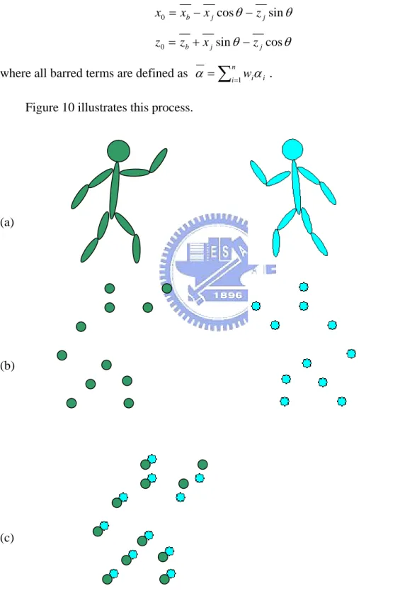
(20) 3. Preprocess Phase The purpose of this phase is to generate a parameter space for later runtime query and joint angular adjustments. The process includes two main steps: 1. Time Alignment. Since motion data are not always well designed and captured, their frame amount or acting speeds may not be the same. This step is to discover temporal relations among the same style of example motions, and then they are time-warped for better blending results. 2. Parameter Extraction and Denser Sampling. We select a representative parameter for each different type of motion. Then various weight combinations are applied to gain more reliable samples for parameter space construction. The remainder of this chapter gives more detailed explanations.. 3.1 Time Alignment We start by aligning a pair of motion. The procedure is done by finding all pairs of “similar” match-frames while keep the order in time. To quantify similarity between two frames, we calculate Euclidean difference between corresponding joints in space domain. So joint representation is converted into a position in world coordinate in advance. We use the distance function proposed by Kovar et al [13] as follow: D ( Fb , F j ) = min. θ , x0 , z 0. ∑. p b ,i − Tθ , x0 , z0 p j ,i. 2. (1). i. where pb ,i and p j ,i are the i th joint of the two motion frames, and T is a transformation which rotates p j ,i by θ degrees about the vertical axis and then translates it horizontally by ( x 0 , z 0 ) .. The transformation T is used to remove the difference of world location between the two frames, and consider only their pose difference. There is a closed-form solution of 11.

(21) Tϑ , x0 , z0 as follows:. ⎛ ∑ wi ( xb ,i z j ,i − x j ,i zb ,i ) − ( xb z j − x j z b ) ⎞ i ⎟ ⎜ ∑ wi ( xb ,i x j ,i + zb ,i z j ,i ) − ( xb x j + xb z j ) ⎟ ⎝ i ⎠. θ = tan −1 ⎜. (2). x0 = xb − x j cos θ − z j sin θ. (3). z 0 = z b + x j sin θ − z j cos θ. (4). where all barred terms are defined as α = ∑i =1 wiα i . n. Figure 10 illustrates this process.. (a). (b). (c). 12.

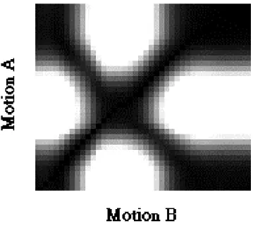
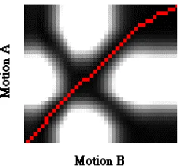
(22) Figure 10: Calculating frame distance. (a) Two motion frames differ in facing direction and location in the world. (b) Representing two motion frames in terms of joint positions. (c) Apply T transformation on one point cloud for pose matching with the other one.. Once the distances of every pair of frames of the two motions have been computed, a grid graph is formed as shown in Figure 11. In this figure, the intensity of cell (x, y) represents the distance between frame x in Motion B and frame y in Motion A. Darker cells represent smaller distances, while lighter ones represent larger distances.. Figure11: A distance grid graph of two motions.. Upon this graph, we look for a minimum cost path starting from the lower left cell to the upper right one. Since time goes forward continuously, the path will only go toward right or up in direction. By this principal, we will find a continuous, and monotonically increasing path with minimal total cost which best time-aligns the two motions. Figure 12 shows the result.. 13.

(23) Figure 12: The path in red shows time alignment between Motion A and Motion B The following two graphs (Figure 13, Figure 14) show two motions in original timing and the result after time alignment.. (a). (b). (c). Figure 13: Motion A (white joint) and Motion B (blue joint) in original timing. (a) Frame 5. (b) Frame 10. (c) Frame 15.. 14.

(24) (a). (b). (c). Figure 14: Time alignment. (a) Frame 9 in Motion A and frame 5 in Motion B. (b) Frame 16 in Motion A and frame 10 in Motion B. (c) Frame 21 in Motion A and frame 15 in Motion B.. Usually there are more than two motions in a motion subject. We have to align them altogether. We select a base motion in a motion subject, and then apply the alignment process to the rest of the entire motion subject. In our experiment, we choose the motion whose attack target is the most general one as the base motion. For example, hit to the front and medium in height, since it is nearly the average of all motions in the same subject. For a punching motion set with N motions, we will get N-1 alignment paths. Figure 15 shows the result.. 15.

(25) (a). (b). Figure 15: Time alignment of a punching motion set. (a) Ready to attack. (b) The attack moment.. 3.2 Parameter Extraction and Denser Sampling Now, we can form a parameter space and its possible attack region. First, we adjust the facing direction of all motions’ ready pose to be as close as the selected base motion, since we would like to get a parameter space for only one ready pose.. Then we pick a joint for each motion subject as the constraint parameter. Because we focus on fighting motions, it is significant to choose the end site of the attack limb. For punching motions, we select the end site of the right arm. For kicking motions, we select the end site of the right leg. After that, we record their attack positions as parameters. So each parameter represents a motion clip that attacks a certain target. These sample parameters can form a convex-hull space. Several of them become the border vertices, others are within the convex hull. Thus we can create reliable motions that attack the targets inside the convex hull. But it is difficult to efficiently estimate for motion from the convex space directly due to the. 16.

(26) sparseness of the convex hull, like the one shown in Figure 7(a).. To gain accuracy, we apply a denser sampling strategy to fulfill the parameter space. New motions are generated by linear interpolation as the following equation.. M new = ∑ wi (c ) M i. (5). i. where c represents a set of blending weight.. We use a constant interval of 0.2 to make a weight group of about a thousand of weight sets. By using these weight combinations, more motions will be created as well as their attack positions. Extracting all parameters makes a denser space, as the figure (Figure 16) shown below:. (a). (b). Figure 16: Denser sampling. Each little red dot represents the motion attack to that position.. When users assign an attack position in the parameter space, a weight set is returned. Blending sample motions using this weight set produces the desired motion. For easier 17.

(27) control, we normalize 3D parameters to a 2D plane.. Obviously, if the sample motions are not well designed and captured, the affine-sum parameter space will be deficient. We take Figure 16(a) as an example. We do not have any motion that punches in the upper-left direction, thus the space looks like a triangle. To our belief, those motions should be synthesized by partial blending. So we find the largest and the smallest values in both horizontal(x) and vertical(y) directions, and extend the possible attack region to the bounding box of the parameter space, as shown in Figure 17. Then, we apply the method describe in the next chapter to synthesis the desired motion.. Figure 17: The white dots represent the original attack space. We extend the space to the red frame. The motions whose parameters are within the red frame can still be synthesized.. 18.

(28) 4. Runtime Phase The parameter space in the previous chapter is constructed by blending the whole body at once. However, it is difficult to create motions attacking the areas that are not in the original parameter space by using the same technique. Motion modifications are needed.. Recall that a martial art action can be regard as a combination of turning the body and attacking at a given height. Usually the orientation of a body pose is mostly dependent on the waist, and the attack height is dependent on the attack limb. Therefore it is plausible to create new motions by rotating joint angles arbitrarily within their predefined limitations, or splicing multiple body segments of different sample motions. By proper joint orientation adjustments, a desired motion can be synthesized. When a user assigns a target parameter, the motion is synthesized by the following approach: 1. Human Body Segmentation. We define several major adjustment joints and divide a human body into several parts. 2. Parameter Query, Body Part Splicing, and Joint Orientation Adjustments. We query two parameters in the original parameter space and discover their correlations to perform reasonable motion adjustments. 3. Motion Length Rearrangement. Due to many-to-one frame matching in time alignment step during the preprocessing phase, the total motion length is longer than the original sample motions. We rearrange motion length to smoothen the synthesized motion.. 4.1 Human Body Segmentation There are two major types of fighting motion — punching and kicking. In general, we define four adjustment joints and segment human body into four parts as well. Figure 18 shows the skeleton we use and how we segment the body. 19.

(29) Y (up ). X (left ). Z ( front ). Figure 18: The human skeleton hierarchy model.. The four partial segments are represented in different colors. The circles are joints, and the brown joints are the defined adjustment joints.. 4.2 Parameter Query, Body Part Splicing, and Joint Orientation Adjustments This step is the major part of this phase. When a user assigns a parameter not in the original space, we apply partial blending and a quick angular adjustment approach to create the desired motion in real-time. Notice that the created motions are still based on the original 20.

(30) parameter space, nevertheless, they are extrapolated by our method.. The following graph (Figure 19) shows the principal idea.. H Adjust. GOAL (b). V (a). (d). (c) Figure 19: Joint angular adjustment.. A motion that punches at upper-left direction (Figure 19(a)) can be regard as: Turn left + Punch toward up Therefore, it can be synthesized by finding a motion that punches at the same height (Figure 19(b)) and a motion that takes left turn with the same angular magnitude (Figure 19(c)).. According to the principal idea, we query two parameters in the original parameter 21.

(31) space to achieve this purpose, as shown in Figure 20:. H. T V. Figure 20: Parameter query for motion synthesis. Given a desired parameter PT , first we want a motion that hits in the same height as we expected. We claim that the attack heights are about the same under the same y parameter, so we query a parameter PH which is closest to PT in horizontal direction. Then we want a motion whose pose turns the same style as the desired target. We claim a turning style is suitable to apply to other motions with various attack height if their x parameters are the same, so we query a parameter PV which is closest to PT in vertical direction.. Now we are going to create the desired motion based on the two queried motions. Notice that there are significant differences in actions and the selected parameter between punching and kicking motion, we divide them into two cases and apply different schemes. Furthermore, we define “right arm” for punching and “right leg” for kicking as the “major active body part”.. Punching Motion There is a high relation between the attack target and the orientation of chest. Imagine 22.

(32) that when a person attacks toward up, his upper body would be straight. On the contrary, when one attacks at a lower target, he may bow his upper body. So it is suitable to blend the target motion M T using the weight set of PH , and adjust the predefined adjustment joints of M H according to the information of M V . We record the following information in advance: The orientation of “Hips” of the first frame of M H and M V . The orientation of “Chest” of the whole motion of M H and M V . The position of “RightCollar” of the whole motion of M H and M V . The position of “End Site” of right arm of the whole motion of M H and M V . We need to compute several variables: All time “Hips” y orientation adjustment jHips . “Chest” y orientation adjustments for each frame jChest _ Y [i ] .. “RightCollar” y orientation adjustments for each frame jRightCollar _ Y [i ] .. Since human body is a hierarchical structure, we apply hierarchical adjustments to “Hips”, “Chest”, and “RightCollar” in order. The orientation adjustments here are specialized in y degree of freedom, as shown in Figure 22.. 23.

(33) (a). (b). (c). (d). Figure 21: Hierarchical adjustments of punching motion.. 24.

(34) θy H's orientation. V's orientation. H’s RightCollar. V’s RightCollar. θy V's End Site. H's End Site. Figure 22: Angular difference of adjustment joints between two motions.. In Figure 21, the desired target is the dot colored in pink, the white dot represents the intermediate result during adjustment. Figure 21(a) is the original queried M H without adjustment. Initially, we compute jHips according to the orientation of “Hips” of the first frame of M H and M V . However, all sample motions are aligned in facing direction of the starting pose, this step only cause a slight adjustment. We apply jHips to create an intermediate result, as shown in Figure 21(b). Then we treat this result as the new M H to compute jChest _ Y [i ] according to the orientation of “Chest” of the whole motion sequence of M H and M V while create another intermediate result, and again treat it as the new M H , as shown in Figure 21(c). Finally, we acquire the vector of the right arm of M H and M V by subtracting the position of “RightCollar” from “End Site”, and compute their angular difference in y degree of freedom as jRightCollar _ Y [i ] , then apply the final adjustment to create the final result shown in Figure 21(d).. It is straightforward to simply adjust the right arm, but it produces unreasonable result. In Figure 23(a), the rotation angle of “RightCollar” exceeds the predefined human joint. 25.

(35) limitation, where Figure 23(b) is our hierarchical adjustment method.. (a). (b). Figure 23: Comparison between adjust right arm directly and hierarchical adjustment.. Kicking Motion Distinct from punching motion, the attack direction is only affected by “Hips” due to the hierarchical structure of human body. As the above-mentioned procedure, there is only a little effect on “Hips” adjustment, unnatural results could be created if using the same scheme as punching motion. In Figure 24, the right leg kicks toward left, but opposite in facing direction.. 26.

(36) Figure 24: Unnatural kicking result by using the adjustment scheme of punching motion.. In this case, we splice the right leg of M H and rest of other parts of M V for proper facing direction of the whole pose. Therefore, “RightHip” is the only adjustment joint of this type of motion. And we record the following information in advance: The position of “Hips” of the whole motion of M H and M V . The position of “RightHip” of the whole motion of M H and M V . The position of “RightKnee” of the whole motion of M H and M V . We also need to compute the following variables: “RightHip” y orientation adjustments of each frame jRightHip _ Y [i ] . “RightHip” x orientation adjustments of each frame jRightHip _ X [i ] .. In Figure 25(a)(c), we acquire the vectors of right leg of M H and M V by subtracting the position of “RightHip” from “RightKnee”, then compute angular difference in y degree of freedom as we did in right arm adjustment. After this step, the direction seems fine, but there are gaps in height. We observed that when one kicks at a higher target, he lifts his right hip, as shown in Figure 26. However, the hip is a critical constraint of the whole motion that we cannot modify it through time. It is difficult to avoid foot-sliding problem if it’s not well 27.

(37) handled. On the other hand, it may take too much computation time to adjust the whole motion if hip adjustment through time is a must, which is against our goal of quick adjustment in real-time.. (a) (b). (c) (d). Figure 25: Right leg orientation adjustment with extra “lift up” or “lay down” for kicking. motion.. Therefore, we compensate the gap at “RightHip” joint. We acquire hip vector by subtracting the position of “Hips” from “RightHip”, then compute their angular differences 「in x degree of freedom」for extra jRightHip _ X [i ] rotation. Thus, the right leg is kicking 28.

(38) higher if the target is high, while kicking lower if the target is low, as shown in Figure 25 (b)(d).. θx. Figure 26: There is an angular difference in the hip vector of motions that kick differs in. height.. 4.3 Motion Length Rearrangement Figure 27 is an example of time alignment. It is obvious to observe the many-to-one frame matching effect. It causes longer and unsmooth result. We shorten the length of the result motion based on M H . A parameter in the original space represents a weight set of sample motions. We find the sample motion which has the largest weight and rearrange the result motion to its length, since M H is more likely to be similar with it than any other sample motions. We take only one iteration of every frame to smoothen the result motion.. Figure 27: An example of time alignment. 29.

(39) 5. Experimental Results 5.1 Environment and Sample Data Our experiments perform on a desktop with a 3.20 GHz CPU, 1.5 GB main memory, and NVIDIA GeForce 6600 graphics card.. There are two punching motion sets and two kicking motion sets as our example data. They are straight punch in seven directions, hook punch in nine directions, straight kick in eight directions, side kick in eight directions. The human skeleton we use contains twenty four joints.. 5.2 Results In this section, we present several result of all four motion sets that attack in various directions.. 30.

(40) Figure 28: Straight punch.. 31.

(41) Figure 29: Hook punch.. 32.

(42) Figure 30: Straight kick.. 33.

(43) Figure 31: Side kick.. 34.

(44) 5.3 Experimental Evaluation and Analysis Evaluation of difference of hit position To evaluate the differences of hit position, we ask a user to assign twenty parameters to each sample data sets randomly, and calculate the differences between the desired parameters and the actual hit parameters. For an actor in 170 centimeters, the difference is measured in centimeters.. Motion Set. Sample. Average. Average. Average. Numbers. Horizontal. Vertical. Difference. Difference. Difference. Straight Punch. 7. 3.55. 0.85. 3.80. Hook Punch. 9. 3.61. 0.51. 3.69. Straight Kick. 8. 2.29. 5.62. 6.42. Side Kick. 8. 2.51. 12.01. 12.95. Table 1: Statistics of hit position difference.. Our method works well on punching motion sets, but it’s not the same as good in kicking motion sets. Actually, we handle the problem of turning behavior better than attacking the desired height. We will talk more in 5.4. Analysis of local joint angle of the spliced joint We utilize the cross validation analysis by taking one of the sample motions away, and forming a parameter space smaller than the original one. Then, we assign the same attack position which is in the original space but not in the newly formed shrunk space. Thus, the former is blended as regular blending while the later is blended and adjusted by our method. We list several examples and illustrate their angle values.. 35.

(45) (a). (b). X Orientation of Chest. X Orientation of RightCollar. partial blending with 8 motions. partial blending with 8 motions. regular interpolation with 9 motions. regular interpolation with 9 motions 1. 50. 0.5 0 Degree. Degree. 40 30 20. -0.5 -1 -1.5 -2. 10. -2.5. 0. Frame. Frame. Y Orientation of RightCollar. Y Orientation of Chest partial blending with 8 motions. partial blending with 8 motions. regular interpolation with 9 motions. regular interpolation with 9 motions 10. 20. 5 0 Degree. Degree. 10 0 -10. -5 -10. -20. -15. -30. -20. Frame. Frame. Z Orientation of RightCollar. partial blending with 8 motions. partial blending with 8 motions. regular interpolation with 9 motions. regular interpolation with 9 motions. 20. 30. 10. 20. 0. 10. Degree. Degree. Z Orientation of Chest. -10 -20. 0 -10 -20. -30 Frame. -30 Frame. Table 2: Hook punch. (a) Regular interpolation with 9 motions. (b) Partial blending with 8. motions. 36.

(46) (a). (b) X Orientation of RightCollar. X Orientation of Chest partial blending with 8 motions. partial blending with 8 motions. regular interpolation with 9 motions. regular interpolation with 9 motions 1. 50. 0 -1. 30. Degree. Degree. 40. 20. -2 -3 -4. 10. -5 -6. 0. Frame. Frame. Y Orientation of Chest. Y Orientation of RightCollar. partial blending with 8 motions. partial blending with 8 motions. regular interpolation with 9 motions. regular interpolation with 9 motions. 15. 10. 10. 5 0. 0. Degree. Degree. 5 -5 -10. -5 -10. -15. -15. -20 Frame. -20 Frame. Z Orientation of Chest Z Orientation of RightCollar. partial blending with 8 motions regular interpolation with 9 motions. partial blending with 8 motions regular interpolation with 9 motions. 15 30. 5. 20. 0. 10. Degree. Degree. 10. -5 -10. 0 -10. -15 Frame. -20 Frame. Table 3: Hook punch. (a) Regular interpolation with 9 motions. (b) Partial blending with 8. motions. 37.

(47) (a). (b). X Orientation of RightHip partial blending with 7 motions regular interpolation with 8 motions 20. Degree. 0 -20 -40 -60 -80. Y Orientation of RightHip. Frame. partial blending with 7 motions. Degree. regular interpolation with 8 motions 20 10 0 -10 -20 -30 -40 -50. Z Orientation of RightHip. Frame. partial blending with 7 motions regular interpolation with 8 motions 10. Degree. 0 -10 -20 -30 -40 Frame. Table 4: Straight kick. (a) Regular interpolation with 8 motions. (b) Partial blending with 7. motions. 38.

(48) (a). (b). X Orientation of RightHip partial blending with 7 motions regular interpolation with 8 motions 20 Degree. 0 -20 -40 -60 -80. Y Orientation of RightHip Frame. partial blending with 7 motions regular interpolation with 8 motions 20 Degree. 0 -20 -40 -60 Frame. Z Orientation of RightHip partial blending with 7 motions regular interpolation with 8 motions 20 Degree. 0 -20 -40 -60 Frame. Table 5: Straight kick. (a) Regular interpolation with 8 motions. (b) Partial blending with 7. motions. 39.

(49) In punching motion examples, we show the local angular values of “Chest” and “RightCollar”. The temporal trends of all values are similar except the medium part of y orientation of “Chest”. The main reason is that we focus on adjusting the upper body of punching motion, there are only slight adjustments at “Hips”. The insufficiency of “Hips” orientation is mostly compensated by “RightCollar”, thus in these two examples, more right turns are taken in that temporal fragment.. In kicking motion examples, we show the local angular values of “RightHip”. It is apparent that the x orientations are shifted down to lift up the right leg additionally. The temporal trends of the medium parts of y and z orientation are much more meaningless due to the large affine transformation differences between global coordinate and the local coordinate of “RightHip” in y and z orientations. However, our adjustments are applied globally.. 5.4 Discussion Our method works better on punching motion sets because they are less affected by the lower body part, and there are several joints between pelvis and the right arm for little by little adjustment. We can change attacking directions by twisting the waist and avoid the problem of root modification.. On the contrary, there is no intermediate joint between pelvis and the right leg, the only joint we can adjust is the “RightHip”. It causes discontinuities in some cases. Imperfect results happen mostly in cases of lifting the right leg up additionally. Our compensation method is not satisfactory to all conditions. The best way to solve this problem is to adjust the hip vector directly, that is, modify “Hips” directly.. However, the pelvis is a critical constraint of motion adjustment. It is the origin of the. 40.

(50) human body hierarchy structure. Any change on it will affect the whole body. The most evident issue is the footskating problem. Though it can be solved by constraining the left foot, the position of the body may change. To smoothen the whole motion sequence, more adjustment has to be put into practice. The computation time is inestimable and real-time requirement cannot be guaranteed.. 41.

(51) 6. Conclusion and Future Work 6.1 Conclusion An efficient example-based method for controlling martial-art motions is presented in this thesis. By parameterizing motion, users could control and produce a motion by simply assign a parameter in the space. By segmenting a human body into parts and apply adjustments to sliced joints individually, motions are extrapolated to new space, and thus enrich the usage of the original imperfect captured data. The adjustment is fast enough to produce new motions for real-time fighting game applications. The proposed approach can deal with not only martial-art motions but also similar motions which can be parameterized.. 6.2 Future Work There are several issues that can be further improved. Our parameter space is downscaled to a 2D plane for simplification. To gain accuracy of the attack position, 3D parameterization may be put into practice. By keeping track of the attack path of a motion rather than a single attack point, a 3D parameter space can be constructed for more possibility of attack positions. Our method does not always conform to kinesiology since it emphasizes more on real-time applications. Physics-based or IK-based approach can be applied for higher motion rationality.. 42.

(52) 7. Reference [1] Al-Ghreimil N., Hahn J. K. 2003. Combined Partial Motion Clips. In WSCG. SHORT PAPERS proceedings, The 11th International Conference in Central Europe on Computer Graphics, Visualization and Computer Vision 2003. [2] Arikan O., and Forsyth D. 2002. Interactive Motion Generation From Examples. ACM Transactions on Graphics, 21, 3, 483-490. [3] Arikan O., Forsyth D. A., and O’Brien J. 2003. Motion synthesis from annotations. ACM Transactions on Graphics 22, 3, 402–408. [4] Arikan O., Ikemoto L., and Forsyth D. A., 2006. Knowing When to Put Your Foot Down. In In ACM SIGGRAPH Symposium on Interactive 3D Graphics 2006, 49-53. [5] Glardon P., Boulic R., and Thalmann D. 2004. A Coherent Locomotion Engine Extrapolating Beyond Experimental Data. In Computer Animation & Social Agents 2004(CASA), 73-84. [6] Gleicher M. 1998. Retargeting Motion to New Characters. In Proceedings Of ACM SIGGRAPH 98, Annual Conference Series, ACM SIGGRAPH, 33-42. [7] Gleicher M., Shin H. J., Kovar L., and Jepsen A. 2003. Snap-Together Motion: Assembling Run-Time Animations. In In ACM SIGGRAPH Symposium on interactive 3D Graphics 2003, 181-188. [8] Grochow K., Martin S. L., Hertzmann A., and Popovic Z. 2004 Style-Based Inverse Kinematics. ACM Transactions on Graphics 23, 3, 522–531. [9] Heck R., Kovar L., and Gleicher M. 2006. Splicing Upper-Body Actions with Locomotion. Computer Graphics Forum(Eurographics 2006 Proceedings)25, 3, 459-466. [10] Ikemoto L., and Forsyth D. A. 2004. Enriching a Motion Collection by Transplanting Limbs. In Proceedings of the 2004 ACM SIGGRAPH/Eurographics Symposium on Computer Animation, 99-108.. 43.

(53) [11] Kovar L., Gleicher M. 2003. Flexible Automatic Motion Blending with Registration Curves. In Proceedings Of ACM SIGGRAPH/Eurographics Symposium on Computer Animation, 214-224. [12] Kovar L., Gleicher M. 2004. Automated Extraction and Parameterization of Motions in Large Data Sets. ACM Transactions on Graphics 23, 3, 559–568. [13] Kovar L., Gleicher M., and Pighin F. 2002. Motion Graphs. ACM Transactions on Graphics 21, 3, 473-482. [14] Mukai T., Kuriyama S. 2005. Geostatistical Motion Interpolation. ACM Transactions on Graphics 24, 3, 1062-1070. [15] Zordan V. B., Majkowska A., Chiu B., Fast M. 2005.Dynamic Response for Motion Capture Animation. ACM Transactions on Graphics 24, 3, 697-701.. 44.

(54)