耐延遲車載網路上利用網路編碼之位置輔助路由 - 政大學術集成

全文

(1)國立政治大學資訊科學系 Department of Computer Science National Chengchi University 碩士論文 Master’s Thesis. 立. 政治大. ‧ 國. 學. 耐延遲車載網路上利用網路編碼之位置輔助路由. ‧. Location assisted Routing with Network Coding in Vehicular Delay Tolerant Networks. n. er. io. sit. y. Nat. al. Ch. hi. en. i n U. gc 研究生：陳界誠指導教授：蔡子傑 . 中華民國一百年一月 January 2011. v.

(2) 耐延遲車載網路上利用網路編碼之位置輔助路由 Location assisted Routing with Network Coding in Vehicular Delay Tolerant Networks. 研究生：陳界誠. Student：Chieh-Cheng Chen. 指導教授：蔡子傑. Advisor：Tzu-Chieh Tsai. 立. 國立政治大學政治資訊科學系碩士論文. 大. ‧ 國. 學 ‧. A Thesis submitted to Department of Computer Science National Chengchi University in partial fulfillment of the Requirements a l for the degree of i v C h Master U n engchi in Computer Science. n. er. io. sit. y. Nat. 中華民國一百年一月. January 2011.

(3) 耐延遲車載網路上利用網路編碼之位置輔助路由摘要. 耐延遲網路(Delay Tolerant Networks)上的路由協定可以區分為兩大類:flooding-based protocols 跟 forwarding-based protocols。. 治政網路編碼(Network Coding)是一種編碼技術可以提高訊息傳輸的可大立 ‧ 國. 學. 靠度；並且運作時不需要知道整體網路的拓樸資訊。. ‧. 我們提出的演算法結合了 flooding-based protocols 跟. sit. y. Nat. forwarding-based protocol 特性，最主要的概念是讓訊息不是被傳. er. io. 送給每一個節點，而是傳送給朝向目的地或是接近目的地的節點。當. n. a. v. l C 節點相遇時，我們的方法會利用節點的路徑、移動方向與速度去預測 ni. hengchi U. 到達目的地的機率。同時我們利用網路編碼的技巧傳送編碼後的資料來代替訊息的片段，來避免重複傳送多餘的訊息；並讓通訊更加可靠。根據實驗模擬的結果，我們的機制有較好的效能，特別是在頻寬的使用上。關鍵字：耐延遲網路、路由協定、網路編碼. i.

(4) Location assisted Routing with Network Coding in Vehicular Delay Tolerant Networks. Abstract The routing protocols of delay tolerant networks could be divided in two categories: flooding-based protocols and forwarding-based protocols. Network coding is an. 立. 治政 encoding technique大that. It operates without the needed of. information about the network topology.. 學. ‧ 國. transmission more reliable.. could make data. ‧. We proposed a routing protocol integrating the characteristic of The main idea. sit. y. Nat. flooding-based protocol and forwarding-based protocol.. of our protocol is to let message would not be flooded to every node but. er. io. n. to the nodes moving atoward or moving closer tov destination.. When. i l C n nodes contact with each other, h eourn gapproach c h i Uwill use the path of node, node’s moving direction and its velocity to estimate the probability to reach the destination of message. At the same time, we exploit network coding to transmit coded block instead of message fragment in order to. avoid sending redundant replication, make data transmit more reliable and more robust to packet losses or delays.. From the result of. simulation, we could see that our protocol have a higher performance especially in the bandwidth consumption compared to other protocols. Keywords: Delay tolerant network, routing, network coding ii.

(5) 致謝辭兩年多的碩士生涯即將結束，此份論文得以完成，必須要感謝很多人的幫助。首先，要感謝我的指導教授，蔡子傑老師。在政大求學的這段日子中，蔡老師對課業或是研究皆熱心地給予許多細心的指導。每當研究進度深陷迷惘停滯不前時，與老師討論之後總是讓我受益良多，才得以找出正確的研究方向繼續前進。若不是老師在研究上的傾力支持，我無法完成這篇論文；也因為老師給予諸多揮灑空間，我才能在撰寫論文時能自由發揮不受限制。另外也要感謝百忙之中抽空前來的口試委員：吳曉光教授、周承復教授與林宗男教授。感謝他們寶貴的意見，點. 政治大. 出這篇論文研究與寫作過程中，未能發現的盲點；並給予我許多建設性的意見。. 立. 並且我也要感謝每一篇我所讀過的論文的作者們，做研究就如同在海上行舟，沒. ‧ 國. 學. 有這些學者孜孜不倦地投入研究工作，不可能勾勒出通往目的地的航海圖。其次，要感謝研究室的所有成員。謝謝勇麟在我車禍骨折後，每天不厭其煩. ‧. 開車送我上下學。謝謝文卿學姊的經驗分享與總是破費請實驗室吃大餐。謝謝泰. y. Nat. sit. 榮與惠翔，常常一起幫忙完成老師交付的每項工作。謝謝欣祺跟貞慈，能與你們. n. al. er. io. 一起口試是我的榮幸。謝謝偉敦每天找我去重訓室，讓我能維持健康的身體。謝. i n U. v. 謝凱禎提供休閑娛樂的材料讓我抒發研究的壓力。謝謝在實驗室一起努力打拼的. Ch. engchi. 思采、英明、昶瑞與欣諦。祝實驗室的各位在未來的日子裡都能身體健康，諸事順利。另外我還要特別感謝宋岳庭的歌曲：Life's a Struggle，在每一個失眠的夜裡陪伴著我。最後，要感謝我的雙親與妹妹，感謝你們多年以來一路包容我的任性、對我所有決定的支持與加油打氣，願意容忍我陰晴不定的暴躁情緒。感謝父母這些年來的養育之恩，也感謝妹妹在我口試之前的關懷與鼓勵。沒有家人的陪伴與無條件付出，就沒有今天的我。此論文得以完成並順利付梓，還有許多未列出的人需要感謝，僅能在此以字句筆墨聊表我心中無限的感激。最後，雖然有點老套，還是不能免俗地說，要感謝的人太多了，不如就感謝國科會吧。 iii.

(6) TABLE OF CONTENTS CHAPTER 1 Introduction.............................................................................................. 1 1.1 Background ................................................................................................ 1 1.1.1 DTNs Routing Protocols ................................................................ 1 1.1.2 Network Coding ............................................................................. 2 1.2 Motivation .................................................................................................. 3 1.3 Organization ............................................................................................... 4 CHAPTER 2 Related Work ........................................................................................... 5 2.1 Flooding-based routing protocol ...................................................................... 6 2.1.1 Direct Contact ....................................................................................... 6 2.1.2 Two-Hop Relay ..................................................................................... 6 2.1.3 Tree-based Flooding.............................................................................. 7 2.1.4 Epidemic Routing ................................................................................. 7 2.2 Forwarding-based routing protocol.................................................................. 8 2.2.1 Location-based Routing ........................................................................ 8 2.2.2 Gradient Routing................................................................................... 8 2.2.3 Link Metrics .......................................................................................... 9 2.3 Flooding-based protocol vs. Forwarding-based protocol ................................ 9 2.4 Random Linear Network Coding ................................................................... 10 2.5 Network Coding on DTNs ............................................................................. 11 CHAPTER 3 The LANC Protocol ............................................................................... 13 3.1 System Model ................................................................................................ 14 3.2 Delivery Probability Estimation .................................................................... 14 3.2.1 Algorithm Path(c) ............................................................................... 15 3.2.2 Algorithm Dir(c) ................................................................................. 17 3.2.3 Algorithm V(c) .................................................................................... 18 3.3 Location-assisted routing with network coding ............................................. 19 3.3.1 Initialization ........................................................................................ 19 3.3.2 Probability Estimation ........................................................................ 20 3.3.3 Coding Operation ................................................................................ 21 3.3.4 Scheduling........................................................................................... 22 3.3.5 Termination ......................................................................................... 24 CHAPTER 4 Simulation and Results .......................................................................... 26 4.1 Performance Evaluation ................................................................................. 26 4.2 Simulation Setup ............................................................................................ 27 4.3 Simulation Results ......................................................................................... 29 4.3.1 Single Flow ......................................................................................... 29 . 立. 政治大. ‧. ‧ 國. 學. n. er. io. sit. y. Nat. al. Ch. engchi. iv. i n U. v.

(7) 4.3.2 Two Flows ........................................................................................... 31 4.3.3 Multiple flows ..................................................................................... 34 CHAPTER 5 Conclusion and Future Work ................................................................. 38 . 立. 政治大. ‧. ‧ 國. 學. n. er. io. sit. y. Nat. al. Ch. engchi. v. i n U. v.

(8) LIST OF FIGURES Figure 1: The concept of network coding ...................................................... 3 Figure 2: Flooding-based protocol vs. Forwarding-based protocol ............. 10 Figure 3: The encoding process of RLNC ................................................... 11 Figure 4: Algorithm Path(c)......................................................................... 15 Figure 5:Calculate Path(c) ........................................................................... 16 Figure 6: Algorithm Dir(c)........................................................................... 17 Figure 7: Calculate Dir(c) ............................................................................ 18 Figure 8: Algorithm V(c).............................................................................. 18 Figure 9: Encoding a single block in source ................................................ 21 Figure 10: Re-encoding in relay .................................................................. 22 Figure 11: The scheduling scheme of LANC .............................................. 23 Figure 12: a snap shop of simulation ........................................................... 27 Figure 13: The parameters of simulation ..................................................... 28 Figure 14: Delivery ratio of single flow ...................................................... 29 Figure 15: Average delay of single flow ...................................................... 30 Figure 16: Overhead ratio of single flow ..................................................... 31 Figure 17: Delivery ratio of two flows ........................................................ 32 Figure 18: Average delay of two flows ........................................................ 33 Figure 19: Overhead ratio of two flows ....................................................... 34 Figure 20: Delivery ratio of varying flow .................................................... 35 Figure 21: Average delay of varying of flow ............................................... 36 Figure 22: Overhead ratio of varying flow .................................................. 37 . 立. 政治大. ‧. ‧ 國. 學. n. er. io. sit. y. Nat. al. Ch. engchi. vi. i n U. v.

(9) CHAPTER 1 Introduction. 1.1 Background. 政治大 The立 purpose is to make communication possible in challenging. Delay tolerant networks or disruption tolerant networks (DTNs) is a kind of special designed network architecture.. The main challenge is that the network lacks of stable, continued end-to-end. ‧ 國. 學. environments.. route paths from source to destination.. Because of these reasons: high node mobility, rapidly. ‧. changing network topology, short transmission range and limited energy resources,. sit. y. Nat. forwarding message in DTNs often suffers frequent disconnection, long-time propagation. n. al. er. io. delay and data losses. A skill called “Store-Carry-Forward” is widely used to overcome the. i n U. v. intermittent connectivity. ”Store-Carry-Forward” works as follow: relay node may store. Ch. engchi. message in buffer for a while and utilize its mobility to carry messages until forwarding message to other relay nodes or even to the final recipient.. 1.1.1 DTNs Routing Protocols There are many routing protocols designed for DTNs based on “Store-Carry-Forward”.. The. main design principle of the routing protocols is trying to make communication possible even if end-to-end connectivity is never achievable.. Maximizing message delivery ratio and. minimizing delay latency is also important criteria needed to be considered.. According to. different strategies properties [1], these routing protocols could be divided into two categories: 1.

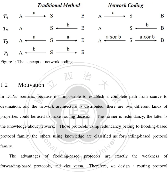
(10) flooding-based protocol and forwarding-based protocol. The flooding-based protocols will duplicate copies of message into network expecting at least one of them received by destination. bandwidth and storage resources.. However, this approach would waste too much. And the forwarding-based protocols require more. information about network to make forwarding decision. But the DTNs is a distributed architecture; it’s difficult for a node to obtain complete network information.. 1.1.2 Network Coding. 立. 政治大. Network coding [2] is a field of information theory and coding theory. With network coding,. ‧ 國. 學. relay nodes may code several input packets into one or several output packets instead of Network coding could make transmission more robustness and. ‧. simply forwarding the data.. sit. y. Nat. adaptability where node and link failures occurs frequently [3], increase throughput gain in. io. er. wireless networks, and operate well without the need of central knowledge about network [4] Exploiting network coding in delay tolerant network is very useful.. n. al. Ch. n U engchi. iv. Because delivering. messages in DTNs often subject to random delay and losses, it’s difficult for a node to select the best packet to send.. With network coding, each node sends coded blocks without. needing any global information about the topology.. Moreover, forwarding random. combination of blocks reduce the probability of sending redundant packet. Figure 1 show the concept of network.. 2.

(11) Figure 1: The concept of network coding. 1.2. 立. Motivation. 政治大. ‧ 國. 學. In DTNs scenario, because it’s impossible to establish a complete path from source to destination, and the network architecture is distributed, there are two different kinds of The former is redundancy; the latter is. y. Those protocols using redundancy belong to flooding-based. sit. Nat. the knowledge about network.. ‧. properties could be used to make routing decision.. n. family. The. al. er. io. protocol family, the others using knowledge are classified as forwarding-based protocol. advantages. of. Ch. i n U. e n g cprotocols hi. flooding-based. forwarding-based protocols, and vice versa.. v. are. exactly. the. weakness. of. Therefore, we design a routing protocol. integrating the concept of the two routing families.. We want message would not be flooded. to every node but to the nodes moving toward or closer to destination. At the same time, we exploit network coding to transmit coded blocks instead of message fragment, in order to avoid sending redundant replication, make data transmit more reliable and more robust to packet losses or delays.. 3.

(12) 1.3 Organization The remainder of this thesis is structured as follows.. Chapter 2 discusses related work about. routing protocols of DTNs and random linear network coding. is described in Chapter 3.. The design of our protocol. Performance evaluation and results are discussed in Chapter 4.. Finally, Chapter 5 summarizes our works and discusses future work.. 立. 政治大. ‧. ‧ 國. 學. n. er. io. sit. y. Nat. al. Ch. engchi. 4. i n U. v.

(13) CHAPTER 2 Related Works. In this chapter, we will discuss other research about the DTNs routing protocols and network coding.. 立. 政治大. First, we introduce the core concepts of flooding-based protocols family and. ‧ 國. 學. forwarding-based protocols family, and then describe the property used by these protocols to make routing decision and conclude their pros and cons.. We will briefly describe the. ‧. n. al. The operation of encoding and decoding process. er. io. technique: random linear network coding.. i n U. of random linear network coding will be described in detail.. Ch. We will illustrate the coding. sit. Nat. The next part is about the research of network coding.. y. operation of each protocol and make a simple summary of these protocols at final.. engchi. v. Finally, we will mention some DTNs routing protocols using network coding similar to our proposed scheme.. 5.

(14) 2.1 Flooding-based routing protocol Redundancy is the key property of this routing category. Protocols in the flooding-based routing family deliver multiple copies of each message to relay nodes, in order to increase the probability that at least one copy will reach destination, or to reduce delivery latency. The advantage of flooding-based routing protocol is that it’s very easy to implement and not needed any information about network topology.. But this approach would consume too. much bandwidth and storage resources and degrade performance.. 立. 2.1.1 Direct Contact. 政治大. ‧ 國. 學. Direct Contact works as follow: The source wouldn’t transmit any data until it comes into. However, the delay latency of message might be the. sit. y. Nat. and it only uses single transmission.. ‧. contact with the destination. Cause of its simplicity, it would not consume many resources,. io. er. longest. It has been proposed that using direct contact to deliver message between mobile nodes and fixed gateways could increase network throughput and decrease resource usage [5].. n. al. Ch. engchi. i n U. v. 2.1.2 Two-Hop Relay In Two-Hop Relay, the source would copy the message to the first n relay nodes that it contacts. There would be n+1 duplicated message in the network, so the probability that message finally delivered to destination is improved n times than direct contact.. This. approach has been used as a backup plan when ordinary ad-hoc routing cannot find a connected path [6].. 6.

(15) 2.1.3 Tree-based Flooding Tree-Based Flooding is an extension of Two-Hop Relay.. The name “Tree-Based Flooding”. comes from that the set of relays forms a tree of nodes rooted at source.. In addition to the. source could make copies of messages, the other relays also do the task of duplicating message.. There would be an index to indicate that how many copies of this message could. be duplicated. Therefore, by appropriately adjusting the index, it would efficiently control. 政治大 If the internodes contact probabilities are identical independent and uniformly 立. the total number of message copies and the farthest hop count from source which it could reach.. distributed, this scheme would achieve optimal performance [7].. ‧. ‧ 國. 學. 2.1.4 Epidemic Routing. y. Nat. io. sit. Replicated databases’ synchronizing is the original purpose of epidemic algorithm [8].. n. al. er. Vahdat and Becjer applied the same concept to deliver data in DTNs [9]. Each message has a unique identifier.. Ch. i n U. It works as follow:. v. When two nodes in contact with each other, they. engchi. would exchange all the identifier numbers in its buffer. If a node finds out that it doesn’t have the identifiers of some messages, it will ask for transmitting these messages it does not have from the contact node.. Eventually, all the nodes will receive the same messages.. Because Epidemic Routing tries every possible contact opportunities to deliver messages over all nodes in the networks, this protocol requires no knowledge about network topology. the delivery latency is minimal if the buffer size is unlimited. benchmark to evaluate the performance in DTNs.. 7. And. Epidemic Routing is also as a.

(16) 2.2 Forwarding-based routing protocol These routing protocols take a more traditional approach to route data in DTNs. Knowledge about network topology is the major property they used to make the best relay selection.. A. relay candidate could be found by using location information, predefined inter contact schedule, historical contact records or assigning metrics to nodes. The advantage is that it reduces unneeded resource consumptions, but it’s hard to obtain complete topology information in a distributed environment with intermittent connectivity.. 立. 2.2.1 Location-based Routing. 政治大. ‧ 國. 學. The Location-based Routing uses positioning services such as GPS (Global Positioning System) to make forwarding decision.. It estimates the probability of delivering messages. ‧. from one node to another by different distance calculating algorithm.. y. Nat. io. sit. each other, they estimate the probabilities before transmitting data.. When nodes contact The advantage of. n. al. er. location-based routing is that it requires very little information about the network. Lebrun et. i n U. v. al. proposed predicting future location of mobile nodes by using motion vector, and proved. Ch. engchi. that it has better delivery ratio than Two Hop Relay and lower overhead than Epidemic Routing [10].. 2.2.2 Gradient Routing The Gradient Routing assigns a weighted value to each node to represent if the node is suitable to deliver message to a given destination. higher weighted value, it passes message to it.. When a node finds another node has So the message follows a gradient of. improving utility function values towards the destination. Compared with Location-based 8.

(17) Routing, this approach requires more information about topology.. First, each mode has to. maintain a metric table for all possible destinations. Second, the metric table must to be propagated to every node to enable each node to compute its probability for all destinations. For example, ZebraNet uses historical records to estimate weighted value [11]. Lindgren et al. propose PROPHET, a probabilistic routing protocol using history of encounter and transitivity [12].. 2.2.3 Link Metrics. 立. 政治大. As traditional network routing protocol, this approach builds a topology graph, assigns. ‧ 國. 學. Therefore, in. order to find best route, this method requires the most network information.. In DTNs, the. ‧. weights to each link and execute a shortest path algorithm to find best path.. sit. y. Nat. weighted value is often determined by the delivery ratio or the delay latency. Jain et al.. io. al. n. schedule [13].. er. present a modified Dijkstra shortest path algorithm based on time-variant with precise. Ch. engchi. i n U. v. 2.3 Flooding-based protocol vs. Forwarding-based protocol We make a simple conclusion for previous mentioned routing protocols and illustrate it in Figure 2. The vertical axis represents the amount of required information about network topology, and the horizontal axis is the degree of redundancy.. It shows that the two routing. categories have the same trend: the more properties it used, the higher delivery ratio it could achieve.. But the efficiency is inversely proportional with the delivery ratio.. 9.

(18) 立. 政治大. ‧ 國. 學. Figure 2: Flooding-based protocol vs. Forwarding-based protocol. ‧. 2.4 Random Linear Network Coding. y. Nat. Radom Linear Network Coding (RLNC) is a form of network coding. RLNC regards the , and all numerical. er. io. sit. messages as vectors of elements in the Galois Field (such as GF 2. operation are also defined on the Galois Field. The RLNC is much more computationally. al. n. v i n C hXORs on incomingU packets. intensive than simply performing engchi. The following illustrates. RLNC operations; consider the source has a message and the message is fragmented into k blocks. ,. ,…,. with the same block size. is generated:. A coded block ∑ The coefficients. · ,. ,…,. is randomly chosen over the GF 2. , where. is called encoding vector, and is transmitted along. with each coded block. Figure 3 shows the encoding process.. 10.

(19) Figure 3: The encoding process of RLNC. 政治大 A node decodes as soon as it立 has received coded blocks X =. ‧ 國. It first forms a. ,…,. with linearly. coefficient matrix C using the. 學. independent encoding vectors.. ,. encoding vectors. Each row in C corresponds to the encoding vectors of one coded block. could be recovered by: X. sit. Nat. B=C. y. ,…,. ‧. ,. The original blocks B. n. al. er. io. The inversion of C is only possible when its rows are linearly independent, in other words C is full rank (rank of C == k).. Ch. engchi. i n U. v. 2.5 Network Coding on DTNs Network coding has been widely used in different network filed. [14, 15] have applied network coding to P2P system.. Several research efforts. Katti et al proposed a scheme to. combine network coding and wireless mesh network [16].. CodeTorrent[17] and. VANETCODE[18] exploit network coding to rapidly distribute data among nodes in vehicular network. There are some routing protocols [19, 20] studied the benefit of network coding on DTNs.. Those protocols applied network coding to avoid redundant replication transmission. 11.

(20) However, those protocols select relay node based on epidemic routing, so they send coded blocks to every contact node results in high transmission overhead.. 立. 政治大. ‧. ‧ 國. 學. n. er. io. sit. y. Nat. al. Ch. engchi. 12. i n U. v.

(21) CHAPTER 3 The LANC Protocol. This section we will introduce our schemes in detail. First we give an overview of the. 政治大 We proposed location-assisted routing. protocol and describe detail in the subsections below.. 立. with network coding: LANC.. The main idea of LANC is, as each contact opportunity. ‧ 國. 學. occurs; calculate the probability of the contact node to check if it is suitable to relay messages to destination.. The criterions we used to estimate probability are trajectory of node, node’s. ‧. moving direction and its velocity. If the result of estimated probability is larger than the. y. Nat. io. sit. threshold, the RLNC operation will be performed on messages in the buffer.. After the. n. al. er. coding process, this protocol schedules messages to transmit according to the estimated results.. i n U. v. When the transmission is completed, the rank map and purge table will be put into. Ch. engchi. beacons to inform other nodes. Once a node receives the beacon from contact node, it could purge its buffer by looking up the purge table.. 13.

(22) 3.1 System Model. We model a DTN as a set of mobile nodes in a vehicular environment. And there is only allowed inter-vehicle communication.. A "contact" is defined as two nodes are within the. radio range of each other, thus they have an opportunity to transfer data. Each node in the network equips global positioning system (GPS) device. installed on every node.. And the navigation system is. The nodes use the navigation system to find a shortest path to its. 政治大 Based on the information provided by navigation system,. destination. The navigation system provides three kind of primitive information: trajectory, moving direction and velocity.. 立. every node can collect navigation information contained in beacon which is broadcasted from. ‧ 國. 學. the contact neighbors during contact time and make routing decision accordingly. The. ‧. destination of message has a fixed location such as a portal to internet. A node can deliver. n. al. er. io. sit. y. Nat. messages to the final recipient directly or via intermediate nodes.. Ch 3.2 Delivery Probability Estimation. engchi. i n U. v. When transmission opportunity occurs during contact time, how to define a delivery quality of node is the first question to address.. Same as the concept of forwarding-based routing. protocol, we use the location information to estimate the delivery probability. First of all, if there is a node that will bring the message closer to destination, we might be able to rely on it to deliver the message.. So we adopt the future trajectory of node. provided by navigation system as one of the estimation factors. However, the trajectory information is not enough to define good relay candidates. For example, a bus may have a fixed trajectory closer to destination but its moving direction is 14.

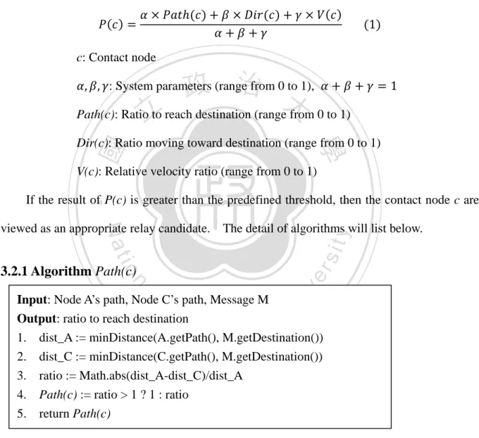
(23) away from it.. Therefore, the node’s moving direction should also take into account.. Finally, it is very intuitive to select a faster node to take the responsibility for delivering message. Combined the three factors, the formula we used to estimate delivery probability listed below: 1 c: Contact node. 政治大 Path(c): Ratio 立to reach destination (range from 0 to 1) , , : System parameters (range from 0 to 1),. 1. ‧ 國. 學. Dir(c): Ratio moving toward destination (range from 0 to 1) V(c): Relative velocity ratio (range from 0 to 1). ‧. If the result of P(c) is greater than the predefined threshold, then the contact node c are. sit. n. al. er. io. 3.2.1 Algorithm Path(c). y. Nat. viewed as an appropriate relay candidate. The detail of algorithms will list below.. Ch. i n U. v. Input: Node A’s path, Node C’s path, Message M Output: ratio to reach destination 1. dist_A := minDistance(A.getPath(), M.getDestination()) 2. dist_C := minDistance(C.getPath(), M.getDestination()) 3. ratio := Math.abs(dist_A-dist_C)/dist_A 4. Path(c) := ratio > 1 ? 1 : ratio 5. return Path(c). engchi. Figure 4: Algorithm Path(c). In algorithm Path(c), the minimal distance between message’s destination and a node’s path is defined as the result that calculating the minimum distance from the location of destination to each coordinates of the path.. For example, in Figure 5 the message is now at node A. 15.

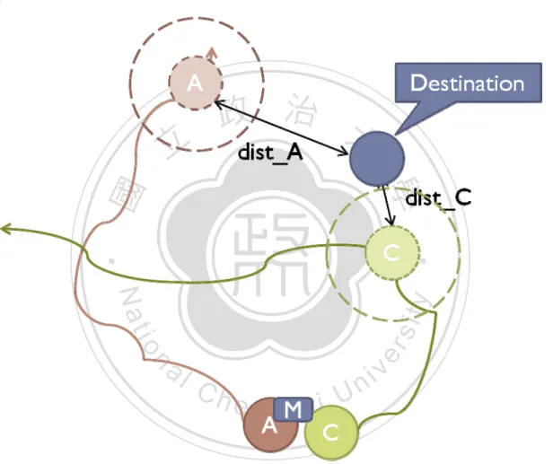
(24) There is a contact node C.. For Node A, the minimal distance between Node A’s future path. and destination is dist_A.. For Node C, the minimal distance from destination to each. coordinates of Node C’s path is dist_C.. It is obvious that node C will be closer to the. destination, so node C is more proper than node A for delivering message M.. Using. algorithm Path(c), we obtain the ratio to reach destination of each contact node.. 立. 政治大. ‧. ‧ 國. 學. n. er. io. sit. y. Nat. al. Ch. engchi. Figure 5: Calculate Path(c). 16. i n U. v.

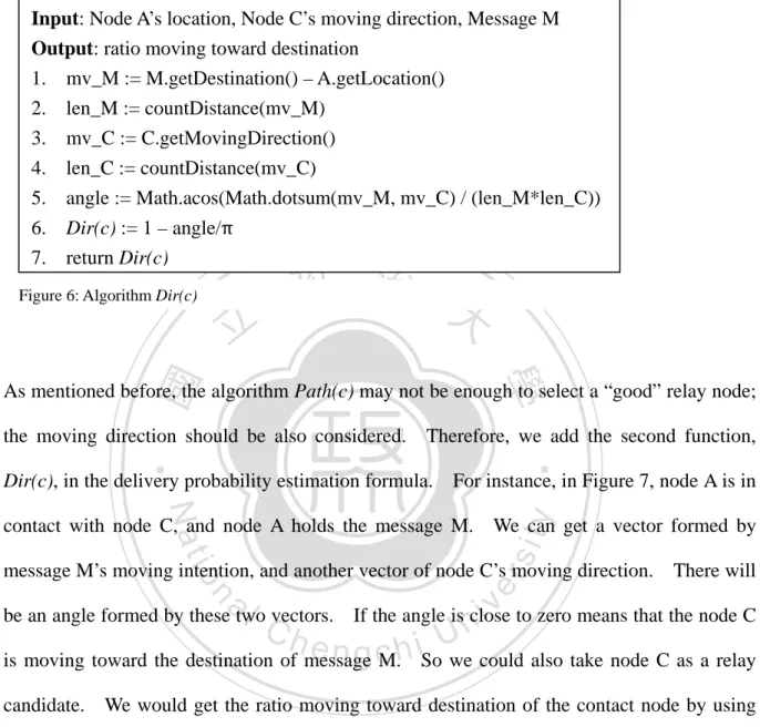
(25) 3.2.2 Algorithm Dir(c) Input: Node A’s location, Node C’s moving direction, Message M Output: ratio moving toward destination 1. mv_M := M.getDestination() – A.getLocation() 2. len_M := countDistance(mv_M) 3. mv_C := C.getMovingDirection() 4. len_C := countDistance(mv_C) 5. angle := Math.acos(Math.dotsum(mv_M, mv_C) / (len_M*len_C)) 6. Dir(c) := 1 – angle/π 7. return Dir(c) Figure 6: Algorithm Dir(c). 立. 政治大. ‧ 國. 學. As mentioned before, the algorithm Path(c) may not be enough to select a “good” relay node; the moving direction should be also considered. Therefore, we add the second function,. ‧. Dir(c), in the delivery probability estimation formula.. For instance, in Figure 7, node A is in. y. Nat. io. sit. contact with node C, and node A holds the message M. We can get a vector formed by. n. al. er. message M’s moving intention, and another vector of node C’s moving direction.. i n U. There will. v. be an angle formed by these two vectors. If the angle is close to zero means that the node C. Ch. engchi. is moving toward the destination of message M. So we could also take node C as a relay candidate. We would get the ratio moving toward destination of the contact node by using algorithm Dir(c).. 17.

(26) 立. 政治大. ‧ 國. 學. Figure 7: Calculate Dir(c). ‧. Nat. Input: Node A’s speed, Node C’s speed Output: relative velocity ratio 1. spd_A := A.getSpeed() 2. spd_C := C.getSpeed() 3. if(spd_C == 0) 4. V(c) := 0 5. else if (spd_A == 0) 6. V(c) := 1 7. else 8. ratio := Math.abs(spd_A-spd_C)/spd_A 9. V(c) := ratio > 1 ? 1 : ratio 10. return V(c). n. al. Ch. engchi. Figure 8: Algorithm V(c). 18. er. io. sit. y. 3.2.3 Algorithm V(c). i n U. v.

(27) When designing a DTN routing protocol, delay latency is an important issue needed to be concerned; hence we wish message delivered to destination as soon as possible. If a node has faster velocity, then it might reach destination quickly. The relative velocity ratio is calculated using algorithm V(c).. 3.3 Location-assisted routing with network coding The LANC 政治大 protocol executes when two nodes are within radio range and have discovered one another. 立 Now we will give a full description of our proposed protocol in this section.. It has five stages: Initialization, Probability estimation, Coding, Scheduling and Termination.. ‧ 國. 學. When two nodes contact with each other, they will collect metadata during initialization After obtain the metadata, the nodes will estimate the delivery probability using the If the result of estimation is larger than. sit. y. Nat. formula we mentioned in previous section 3.2.. ‧. stage.. io. er. threshold, it will perform coding operation on the messages in outgoing buffer. Due to not all the coded blocks are needed to be delivered, the coded blocks will be scheduled by the. al. n. v i n C h node’s rank map.U After the transfer is finished, if the previous estimated results and contact engchi. receiver is the destination of the message, it will try to decode the message, update purge table or rank map depending on the decoding result. The detail of each stage is listed below.. 3.3.1 Initialization When moving in the networks, nodes will send out periodic beacons which allow detecting contact nodes in the transmission range. A node will not send out any message if it has no neighbors. The beacons not only inform neighbor the presence of node, but also contain the metadata of node. 19.

(28) The metadata contained in beacon includes: trajectory information of node, node’s moving direction, velocity, rank map and purge table.. The first three factors are used to. estimate delivery probability as we mentioned before. independent encoding vectors of each message.. The rank map is a record of. The purge table indicates which message. has already decoded. The format of rank map is: (M_ID: R, M_ID: R, M_ID: R …) M_ID: unique id of message. 政治大 In order to distinguish a coded block belongs to which message, a unique identifier will 立 R: rank of message. called SHA-1 to generate unique identifier for each message.. 學. ‧ 國. be assigned to message before encoding process at source. Here we use a hash function. ‧. The rank of message is the number of independent encoding vectors.. At each. sit. y. Nat. transmission finished, a node will check the rank of message, and records the value with. io. er. corresponding message identifier.. The format of purge table is: (M_ID: T, M_ID: T, M_ID: T…). n. al. Ch. M_ID: unique id of message. engchi. i n U. v. T: the time original message is decoded. If the original message is decoded successfully, its identifier and the time decoding process finished will be pushed into the purge table and propagated by beacons.. Nodes. receive this beacon could drop coded blocks according to the same identifier to release memory space.. 3.3.2 Probability Estimation After discovering a contact node by its beacon, a node could estimate the delivery probability 20.

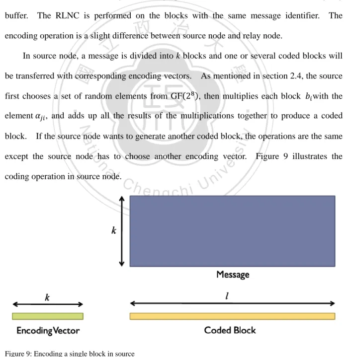
(29) using the formula we mentioned in section 3.1.. The procedure works as follow: for each. message in buffer, if the result of P(c) is larger than threshold, then puts the message in outgoing buffer for next coding stage.. 3.3.3 Coding Operation Before the transmission starting, the coding operation will code the blocks in the outgoing buffer. The RLNC is performed on the blocks with the same message identifier. The. 政治大. encoding operation is a slight difference between source node and relay node.. 立. be transferred with corresponding encoding vectors.. 學. ‧ 國. In source node, a message is divided into k blocks and one or several coded blocks will As mentioned in section 2.4, the source. first chooses a set of random elements from GF 2 , then multiplies each block. , and adds up all the results of the multiplications together to produce a coded. y. Nat. If the source node wants to generate another coded block, the operations are the same. io. sit. block.. ‧. element. with the. n. al. er. except the source node has to choose another encoding vector. Figure 9 illustrates the coding operation in source node.. Ch. engchi. Figure 9: Encoding a single block in source 21. i n U. v.

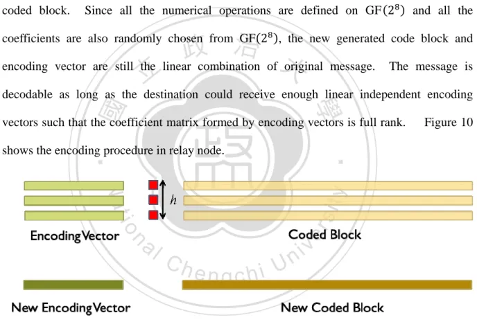
(30) If a relay node wants to send coded blocks to another node, it operates similar operations as source does. It also chooses a set of random elements from GF 2 , but the size of this set is the number of coded blocks with the same message identifier in its buffer.. Relay node. multiplies each element with encoding vector and finally adds up to produce a new encoding vector.. This operation is repeated again using the same set of elements to generate a new. coded block.. Since all the numerical operations are defined on GF 2. 政治大 encoding vector are still the linear combination of original message. 立. and all the. coefficients are also randomly chosen from GF 2 , the new generated code block and The message is. decodable as long as the destination could receive enough linear independent encoding. ‧ 國. 學. vectors such that the coefficient matrix formed by encoding vectors is full rank.. ‧. shows the encoding procedure in relay node.. Figure 10. n. er. io. sit. y. Nat. al. Ch. engchi. i n U. v. Figure 10: Re-encoding in relay. 3.3.4 Scheduling Before starting a transmission, we will schedule which coded blocks in outgoing buffer should be transferred first to get better performance.. As we mentioned in previous section, a. message is decodable only if its encoding matrix is full rank. Therefore, the rank of message is the first factor we used to make scheduling decision. During initialization stage, a node 22.

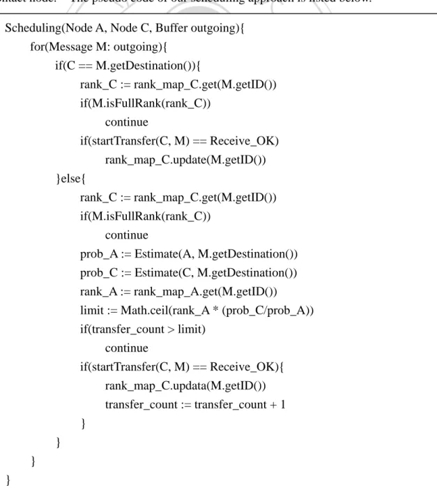
(31) could obtain the contact node’s rank map from beacon.. Then the node could look up the. rank map of contact node by message identifier to get the corresponding rank. The second factor is the delivery probability to destination. In section 3.2, we proposed our method to estimate the probability if the contact node would reach the destination in the future.. So the probability can be regarded as the power that delivering messages to the final. recipient. With great power comes great responsibility. If a node finds out that the power of its contact node is less than its power, this node would not have to transfer all the coded. 政治大 The pseudo code of our scheduling approach is listed below. 立. blocks to its contact node. to contact node.. It will merely transfer part of coded blocks in its outgoing buffer. ‧. ‧ 國. 學. Scheduling(Node A, Node C, Buffer outgoing){ for(Message M: outgoing){ if(C == M.getDestination()){ rank_C := rank_map_C.get(M.getID()) if(M.isFullRank(rank_C)) continue if(startTransfer(C, M) == Receive_OK) rank_map_C.update(M.getID()) }else{ rank_C := rank_map_C.get(M.getID()) if(M.isFullRank(rank_C)) continue prob_A := Estimate(A, M.getDestination()) prob_C := Estimate(C, M.getDestination()) rank_A := rank_map_A.get(M.getID()) limit := Math.ceil(rank_A * (prob_C/prob_A)) if(transfer_count > limit) continue if(startTransfer(C, M) == Receive_OK){ rank_map_C.updata(M.getID()) transfer_count := transfer_count + 1 } } } 23 }. n. er. io. sit. y. Nat. al. Ch. engchi. Figure 11: The scheduling scheme of LANC. i n U. v.

(32) 3.3.5 Termination A transfer ends when two nodes are out of radio range or all outgoing blocks transmitted. After the transfer, the node which received coded blocks would update the rank map, or try to recover the original message by decoding.. 3.3.5.1 Update Rank Map After receiving a coded block, a node will execute Gaussian elimination procedure to verify if. 政治大. the incoming coded blocks is innovate to the coded blocks in buffer.. 立. If the result of. checking is true, the incoming coded block will be put into buffer and increase the rank. ‧ 國. 學. counter by one in rank map according to the message identifier.. ‧. 3.3.5.2 Decoding. sit. y. Nat. After the rank map updating, if the encoding matrix of message is full rank, in other words,. n. al. er. io. the number of independent encoding vector equals the size of each single encoding vector, the. i n U. v. Gaussian elimination will be operated on it to get the inverse of encoding matrix.. Ch. engchi. The. original message will be recovered by encoding the inverse of encoding matrix and coded block.. 3.3.5.3 Update Purge Table In DTNs, some nodes would continuously send the messages that have already delivered to destination because these nodes don’t know the messages reached their final recipient. To ease the kinds of redundant transmissions and buffer occupancy, once the destination recovers the original message successfully by decoding operation, the purge table will be updated by adding the message identifier and the time it decoded. The purge table will be propagated by beacons over the network.. After received the beacons, a node will compare 24.

(33) the message identifiers contained in purge table with messages identifier of coded blocks currently stored in its buffer.. If it finds out the same identifier, it will purge the buffer by. discarding the coded blocks with the same message identifier immediately because it is not necessary to send the coded blocks of this message anymore.. 立. 政治大. ‧. ‧ 國. 學. n. er. io. sit. y. Nat. al. Ch. engchi. 25. i n U. v.

(34) CHAPTER 4 Simulation and Results. This section we will discuss the simulation.. We evaluate the performance of LANC through. 政治大. simulation by using the Opportunistic Network Environment simulator [21].. 學. ‧ 國. 立. 4.1 Performance Evaluation. The main object of a DTN routing protocol is to maximize the message delivery ratio and to. ‧. minimize the delay latency.. We evaluated our protocol in vehicles environment.. y. Nat. n. al. er. io. Message delivery ratio. . Average delay latency. . Transmission overhead:. sit. evaluate the performance of LANC using three metrics: . We. Ch. engchi. i n U. v. The transmission overhead is defined as. We compare LANC with another two routing protocols: Epidemic Routing and PROPHET Routing.. The Epidemic Routing is a greedy approach that duplicates copies of. message to every contact node. The PROPHET Routing uses history of encounter and transitivity to select a better relay node.. We modified these two protocols such that they. have the ability to perform random linear network coding. 26.

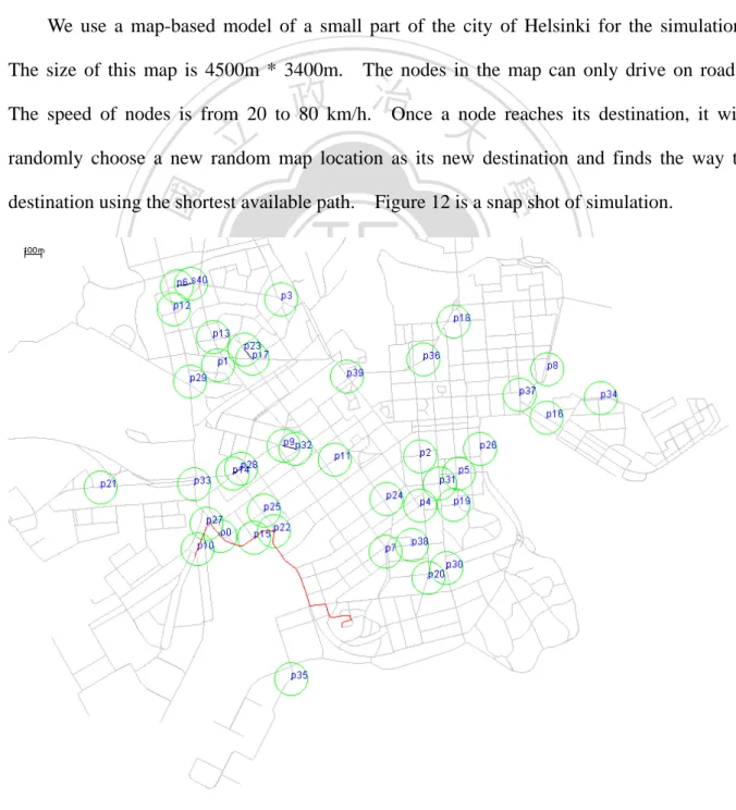
(35) 4.2 Simulation Setup Our evaluations are based on The ONE (Opportunistic Network Environment simulator), a simulator written in java.. We developed a set of extensions to the simulator to enable. nodes could overhear neighbors’ transmissions and to implement a random linear network coding module. We use a map-based model of a small part of the city of Helsinki for the simulation. The size of this map is 4500m * 3400m. The nodes in the map can only drive on roads.. 政治Once a大node reaches its destination, it will. The speed of nodes is from 20 to 80 km/h.. 立. destination using the shortest available path.. 學. ‧ 國. randomly choose a new random map location as its new destination and finds the way to Figure 12 is a snap shot of simulation.. ‧. n. er. io. sit. y. Nat. al. Ch. engchi. Figure 12: a snap shot of simulation 27. i n U. v.

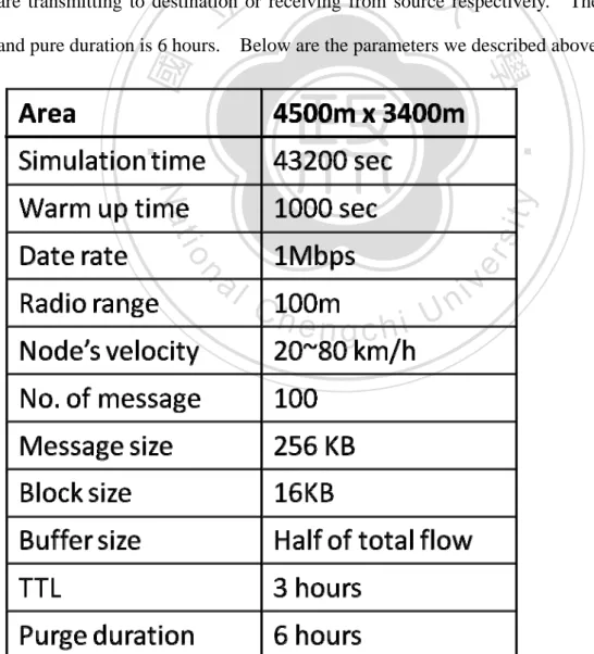
(36) The simulation times are 43200 seconds. seconds.. For the fairness, the warm up time is 1000. The nodes only could move but not allow transmitting any message until the warm. up time counts down to zero.. Each destination of flow has a stationary location selected. randomly before starting the simulation.. Every node has only one single network interface.. The data rate is 1 Mbps and the transmission range is 100m.. For each flow, there are 100. messages to transmit. Each message is divided into 16 blocks. The size of a message is 256KB, so the size of each block is 16KB.. The buffer size of every node is set to half of. 政治大 are transmitting to destination or receiving from source respectively. 立. total flow, but the source and destination have additional buffer space to store message that. and pure duration is 6 hours.. Below are the parameters we described above.. ‧. ‧ 國. 學. n. er. io. sit. y. Nat. al. The TTL is 3 hours,. Ch. engchi. Figure 13: The parameters of simulation 28. i n U. v.

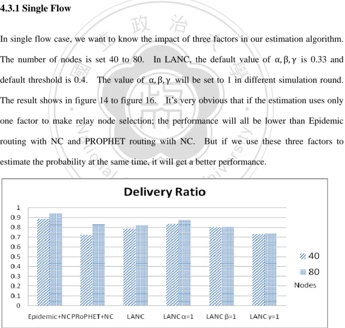
(37) 4.3 Simulation Results We evaluated our approaches in three different scenarios: single flow, two flows and multiple flows.. Although our protocol has a little higher data transmission delay than other protocols,. but the delivery ratio is almost the same as Epidemic routing with NC in multiple flows scenario.. It shows that with overhead ratio, LANC outperforms with other approaches.. 4.3.1 Single Flow. 政治大 In single flow case, we want to know the impact of three factors in our estimation algorithm. 立 The number of nodes is set 40 to 80.. In LANC, the default value of α, β, γ is 0.33 and. ‧ 國. 學. default threshold is 0.4. The value of α, β, γ will be set to 1 in different simulation round.. ‧. The result shows in figure 14 to figure 16. It’s very obvious that if the estimation uses only. But if we use these three factors to. io. er. routing with NC and PROPHET routing with NC.. sit. y. Nat. one factor to make relay node selection; the performance will all be lower than Epidemic. estimate the probability at the same time, it will get a better performance.. n. al. Ch. engchi. Figure 14: Delivery ratio of single flow. 29. i n U. v.

(38) From figure 14, the future trajectory information of a node is the most significant factor for increasing delivery ratio.. The reason is that even if the relay node couldn't reach the. destination eventually, the other nodes around destination could take over the responsibility of delivering message to final recipient. Therefore, a message should be transferred to the node has the minimal distance between its future trajectory and the destination of message.. 政治大. 立. ‧. ‧ 國. 學 er. io. sit. y. Nat Figure 15: Average delay of single flow. n. al. Ch. engchi. i n U. v. We could get the same conclusion as figure 14 from figure 15. destination, the less time it needs to reach destination.. If a message is closer to. On the contrary, if the message is. taken away from its destination, it has to do more effort to get back to destination, and it’s very time-consuming.. And if the estimation function only considers the velocity of contact. node, it may make an inappropriate selection. The contact node has the higher speed does not guarantee it will reach the destination sooner or has higher delivery ratio. moving direction might be away from destination.. 30. Because its’.

(39) Figure 16: Overhead ratio of single flow. 立. 政治大. ‧ 國. 學. From figure 16, we can get another conclusion that the overhead ratio could be decreased by estimating the moving direction of the contact node.. In figure 16, Epidemic routing with NC. ‧. 1 has the second large overhead ratio.. io. sit. Nat. of a contact node. The LANC with γ. y. has the largest overhead ratio since the protocol has no ability to estimate the delivery power Because. n. al. er. there are lots of nodes in the network, and the velocity difference between two nodes may be very large results a poor estimation.. Ch. engchi. i n U. v. 4.3.2 Two Flows In two flows scenario, we want to understand the effect of scheduling. We will compare our scheduling with the ordinary FIFO scheduling and Random scheduling. The estimation function of PROPHET routing with NC is based on historical records of encounter.. Since. the Epidemic routing with NC simply forward message to every contact node, we assign the value to 1 as the result after estimation.. 31.

(40) 政治大. 立. ‧ 國. 學. Figure 17: Delivery ratio of two flows. ‧ y. sit. n. al. er. This is because the schedule scheme considers the rank map and the probability to the. io. ratio.. Nat. From figure 17, it’s clear that the schedule approach we propose could increase the delivery. i n U. v. destination. If a message is full rank, then it should give the transmission opportunity to the. Ch. engchi. next message which is not full rank. Therefore, the delivery ratio is almost twice compared with ordinary FIFO scheme.. 32.

(41) 政治大. 立. ‧ 國. 學. Figure 18: Average delay of two flows. ‧. sit. y. Nat. In figure 18, the difference of delay latency between our schedule and ordinary FIFO is about. io. er. 200 to 250 seconds. According to the same reason, our schedule scheme will balance the responsibility of delivering message by estimating the probability to destination.. n. al. Ch. n U engchi. iv. Therefore,. it would select proper relay candidates to take the responsibility to delivery coded blocks. In FIFO scheme, it schedule coded blocks to send by the time which blocks arrived. Hence, some message may suffer starvation.. 33.

(42) 立. 政治大. ‧ 國. 學. Figure 19: Overhead ratio of two flows. ‧ y. Nat. io. Before sending coded blocks to contact node, our approach will estimate the. n. al. er. consumptions.. sit. From figure 19, it’s obvious that our schedule scheme could large save bandwidth. delivery probability of the contact node. ordinary FIFO scheme.. Ch. i n U. v. Hence, the result of overhead ratio is better than. engchi. Moreover, the accuracy of estimation is higher in LANC, so the. overhead ratio is much smaller than other approaches.. 4.3.3 Multiple flows The final case is multiple flows.. We adjust the number of flows from 6 to 10.. Figure 21. shows that the performance of each protocol drops down with the load of flow increase.. 34.

(43) 政治大. 學. ‧ 國. 立 Figure 20: Delivery ratio of varying flow. ‧. Once there are more flows in the network, congestion might occur at some bottleneck relay Our protocol uses purge table to inform other node to purge its buffer, this operation. sit. y. Nat. node.. n. al. er. io. not only frees memory storage but also reduces the chance the congestion occurs. Moreover,. i n U. v. LANC uses rank map to schedule the priority of coded blocks.. Ch. engchi. If a message is already full. rank, LANC will bypass the opportunity to next message.. At the same time, LANC views the results of estimation function as the probability a node would future move toward the destination, LANC could schedule coded blocks according the probability to decide deliver it to another or not, so the responsibility for delivering message could be shared by a set of nodes. If a relay node would never reach the destination in the future, it won’t be a problem hence the node doesn’t have all the coded blocks.. 35.

(44) 學. ‧ 國. 立. 政治大. Figure 21: Average delay of varying of flow. The LANC has a little higher delay. y. The difference is about 1200 seconds.. For non-real. sit. Nat. time than Epidemic routing with NC.. ‧. The average delay increases with the trend of flow load.. n. al. er. io. time demand such as sending emails or uploading photos, it’s considered acceptable. And. i n U. v. Epidemic routing tries every possible contact opportunities, the network bandwidth it wasted must be very large.. Ch. engchi. In other words, our protocol is more efficient because the bandwidth. consumed by LANC is less. As for PROPHET routing with NC, the estimation it made is based on historical encounter record, so it has a poor result. The method PROPHET routing used might be suitable for a small closed area like a concert or a lounge bar. Because LANC uses the future possible trajectory of node to predict the delivery probability, LANC could make more precise estimation in large scale outdoor environment.. 36.

(45) 政治大. 學. ‧ 國. 立 Figure 22: Overhead ratio of varying flow. ‧. The overhead ratio of our approach is much smaller than Epidemic routing with NC and. n. al. Although it will keep the coded. er. io. coded block, hence our protocol require less transmissions.. sit. y. Nat. PROPHET routing with NC. The LANC will select “better” relay candidates to deliver. i n U. v. blocked in buffer for a while, the purge mechanism will ease the situation.. Ch. engchi. 37.

(46) CHAPTER 5 Conclusion and Future Work. Conclusion. 政治大 schedules message to transmit 立 when contact opportunity occurs.. In this thesis, we proposed LANC which estimates the probability to the destination and Moreover, in LANC, we. ‧ 國. 學. exploit network coded data transmissions in DTNs; making messages transmission between mobile nodes more robust to random data delays and losses. In simulation, we could see that. ‧. with different scenarios, LANC could achieve good performance, especially in bandwidth. n. al. er. io. sit. y. Nat. consumption.. Future Work. Ch. engchi. i n U. v. In this thesis, we assumed nodes in network have part of information about network and the destination of each flow is stationary.. In future works, we try to verify it.. The estimation. factor we used is the path of node, path’s moving direction and its velocity. For future work, we will estimate the probability with more network conditions, such as contact duration. Moreover, we want to perform our work in real scenarios on mobile handheld device. Finally, we would try to apply our work to other more complicated DTN scenarios.. 38.

(47) Reference [1] Jian Shen, Sangman Moh, and Ilyong Chung, “Routing Protocols in Delay Tolerant Networks: A Comparative Survey” in International Technical Conference on Circuits/Systems, Computers and Communications (ITC-CSCC’ 08), July 2008 [2] R. Ahlswede, N. Cai, S.-Y. R. Li, and R.W. Yeung, “Network information flow,” IEEE Trans. on Information Theory, vol. 46, no. 4, July 2000. [3] T. Ho, R. Koetter, M. Medard, D. R. Karger, and M.Effros. “The benefits of coding over routing in a randomized setting”International Symposium on Information Theory (ISIT), page 442, July 2003. 立. 政治大. [4] P. A. Chou, Y. Wu, and K. Jain. Practical network coding. In Proc. Allerton, Oct. 2003.. ‧ 國. 學. ‧. [5] R. H. Frenkiel, B. R. Badrinath, J. Borres, and R. D. Yates, “The infostations challenge: balancing cost and ubiquity in delivering wireless data,” IEEE Personal Communications, vol. 7, no. 2, pp. 66–71, 2000. y. Nat. [6] D. Nain, N. Petigara, and H. Balakrishnan,“Integrated routing and storage for messaging. sit. n. al. er. io. applications in mobile ad hoc networks,” Mobile Networks and Applications (MONET), vol. 9, pp. 595–604, December 2004.. Ch. i n U. v. [7] T. Spyropoulos, K. Psounis, and C. S. Raghavendra,“Spray and wait: an efficient routing. engchi. scheme for intermittently connected mobile networks,” in Proceedings of the ACM SIGCOMM Workshop on Delay-Tolerant Networking (WDTN’05), pp. 252–259, August 2005. [8] A. Demers, D. Greene, C. Houser, W. Irish, J. Larson, S. Shenker, H. Sturgis, D. Swinehart, and D. Terry,“Epidemic algorithms for replicated database maintenance,” SIGOPS Operating Systems Review, vol. 22, pp. 8–32, January 1988. [9] A. Vahdat and D. Becker, “Epidemic routing for partially-connected ad hoc networks,” Tech. Rep. CS-2000-06, Duke University, July 2000. [10] J. Lebrun, C.-N. Chuah, D. Ghosal, and M. Zhang,“Knowledge-based opportunistic forwarding in vehicular wireless ad hoc networks,” in Proceedings of. 39.

(48) IEEE Vehicular Technology Conference (VTC), vol. 4, pp. 2289–2293, May 2005. [11] P. Juang, H. Oki, Y. Wang, M. Martonosi, L. S. Peh, and D. Rubenstein, “Energy-efficient computing for wildlife tracking: design tradeoff’s and early experiences with zebranet,” in Proceedings of ASPLOS-X, pp. 96–107, October 2002. [12] A. Lindgren, A. Doria, and O. Schel´en, “Probabilistic routing in intermittently connected networks,” Lecture Notes in Computer Science, vol. 3126, pp. 239–254, January 2004. [13] S. Jain, K. Fall, and R. Patra, “Routing in a delay tolerant network,” in Proceedings of ACM SIGCOMM, vol. 34, pp. 145–158, ACM Press, October 2004.. 政治大. [14] C. Gkantsidis and P. Rodriguez. Network coding for large scale content distribution. In Infocom, Miami,FL, Mar. 2005.. 立. ‧ 國. 學. [15] C. Gkantsidis, J. Miller and P. Rodrques. Comprehensive view of a live network coding P2P system. sit. Nat. Practical Wireless Network Coding. In SIGCOMM, 2006.. y. ‧. [16] S. Katti, H. Rahul, D. Katabi, W. Hu M. M´edard, and J. Crowcroft. XORs in the Air:. er. io. [17] U. Lee, J.-S. Park, J. Yeh, G. Pau, and M. Gerla. “CodeTorrent: Content Distribution using Network Coding in VANETs. “ in MobiShare’06, Los Angeles, CA, Sept. 2006.. al. n. v i n C“VANETCODE: [18] S. Ahmed and S. S. Kanhere, h e n g c h Network i U coding to enhance cooperative downloading in vehicular ad-hoc networks,” in Proc. ACM Int. Conf. on Commun. And Mobile Comput., 2006, pp. 527–532.. [19] J. Widmer and J.-Y. LeBoudec. “Network coding for efficient communication in extreme networks. “ in WDTN, Aug. 2005. [20] X. Zhang, G. Neglia, J. Kurose, D. Towsley. “On the Benefits of Random Linear Coding for Unicast Applications in Disruption Tolerant Networks. “ in Second Workshop on Network Coding, Theory, and Applications. 2006 [21] A. Keränen, J. Ott, and T. Kärkkäinen, "The ONE Simulator for DTN Protocol Evaluation," in SIMUTools'09: 2nd International Conference on Simulation Tools and Techniques, Rome, March 2-6, 2009. 40.

(49)