Boundary Effects on Diffusiophoresis and Electrophoresis: Motion of a Colloidal Sphere Normal to a Plane Wall

(1)

ARTICLE NO. 0569

Boundary Effects on Diffusiophoresis and Electrophoresis:

Motion of a Colloidal Sphere Normal to a Plane Wall

HUANJ. KEH1ANDJENGS. JAN

Department of Chemical Engineering, National Taiwan University, Taipei 106-17, Taiwan, Republic of China

Received April 23, 1996; accepted July 2, 1996

field ( such as electrical potential, temperature, or solute

con-A combined analytical – numerical study of the diffusiophoresis _{centration ) that interacts with the surface of each particle.} and electrophoresis of a rigid sphere in a uniform applied field

A good review of particle motions associated with this

mech-perpendicular to a plane wall is presented. The range of the

inter-anism, known as ‘‘phoretic motions,’’ was given by

Ander-action between the solute species and the solid surfaces is assumed

son ( 1 ) .

to be small relative to the particle’s radius and to the spacing

Perhaps the most familiar example of the various phoretic

between the particle and the wall, but the polarization of the

dif-motions of colloidal particles is electrophoresis, which

re-fuse species in the thin particle – solute interaction layer is allowed.

sults from the interaction between an applied electric field

A slip velocity of fluid and normal fluxes of solute species at the

and the electrical double layer surrounding a charged

parti-outer edge of the thin diffuse layer are used as the boundary

conditions for the fluid domain outside the diffuse layer. Through cle. The electrophoretic velocity U0of a single

nonconduct-the use of a collocation method along with nonconduct-these boundary condi- _{ing particle suspended in an unbounded fluid is related to} tions, a set of conservative equations governing the system is solved _{the uniformly applied electric field E}` _{by the well-known} in the quasisteady state situation and the effects of a plane wall _{Smoluchowski equation ( 2 – 4 ) ,}

on diffusiophoresis and electrophoresis are calculated for various cases. For the cases of diffusiophoresis in a nonelectrolyte gradient

and of electrophoresis, the particle velocity decreases monotoni- _U0 _Å ez

4phE

`_. _[1.1]

cally with the decrease of the distance of the particle center from the wall. For the case of diffusiophoresis in an electrolyte gradient, however, the boundary effect is a complicated function of the

Here, e / 4p is the fluid permittivity, h is the fluid viscosity,

properties of the particle and ions, and it no longer varies

monoton-and z is the zeta potential associated with the particle surface.

ically with the separation distance for some situations. q 1996

Another example of phoretic motions is called

‘‘diffusio-Academic Press, Inc.

phoresis’’ ( 4 ) , which is the migration of a solid particle

Key Words: diffusiophoresis; electrophoresis; boundary effect;

in response to the macroscopic concentration gradient of a

thin but polarized diffuse layer.

molecular solute; the solute can be nonionic or ionic. The particle moves toward or away from regions of higher solute concentration, depending on long-range interactions between

1. INTRODUCTION

the solute molecules and the particle. In an unbounded solu-The transport behavior of small particles in a continuous tion with a constant concentration gradient Ç_n`_{, the}

medium at low Reynolds numbers is of much fundamental diffusiophoretic velocity of a particle is and practical interest. In general, driving forces for motions

of colloidal particles include concentration gradients of the

U0ÅkT

h L * KÇn

` _{[1.2 ]}

particles themselves ( diffusion ) , bulk velocities of the dis-perse medium ( convection ) , and gravitational or centrifugal fields ( sedimentation ) . Problems of the colloidal transport

for the case of a nonionic solute ( 5 ) , and induced by these well-known driving forces have been

treated extensively in the past. Another category of driving forces for the locomotions of colloidal particles, which has

U0Å ez 4ph kT Ze Ç_n` n`( 0 )

F

D20D1 D2/D1 / 4kT Zez ln cosh

S

Zez 4kT

DG

commanded less attention, involves a nonuniform imposed

1

(2)

for the case of a symmetric electrolyte solute ( 6 ) . Here, L * and is a characteristic length for the range of particle – solute

interactions, K is the Gibbs adsorption length characterizing _D_Å 1

a2( a 2

/ab11/ab22/b11b220b12b21) , [1.6 ] the strength of the adsorption ( K and L * are defined by

Eqs. [ 3.3a ] and [ 3.3d ] ) , n`( 0 ) is the macroscopic solute

where b11, b12, b21, and b22 are relaxation coefficients de-concentration measured at the particle center 0 in the absence

fined by Eq. [ 2.6 ] or [ 4.3 ] . IfÉzÉis small and ka is large, the

of the particle, D1 and D2 are the diffusion coefficients of

interaction between the diffuse counterions and the particle the anion and cation, respectively, Z is the absolute value

surface is weak and the polarization of the double layer is of the valences of the ions, e is the charge of a proton, k is

also weak. In the limit of the Boltzmann constant, and T is the absolute temperature.

Equations [1.1] – [1.3 ] indicate that the electrophoretic

and diffusiophoretic velocities of a particle are independent _{( ka )}01

exp

S

ZeÉzÉ

2kT

D

r 0, [1.7 ] of particle size and shape. However, their validity is based

on the assumptions that the local radii of curvature of the

c1 Åc2Å 0.5 ( b11/ a Åb12/ aÅ b21/ a Åb22/ aÅ 0 ) and particle are much larger than the thickness of the particle –

Eq. [1.4 ] reduces to the Smoluchowski equation [1.1] . solute interaction layer at the particle surface and the effect

For the case of diffusiophoretic motion of a colloidal of the polarization ( relaxation effect ) of the diffuse solute

sphere with a thin but polarized particle – solute interaction species in the interfacial layer due to nonuniform ‘‘osmotic’’

layer in a gradient of nonelectrolyte solute, the formula for flow is negligible. Recently, important advances have been

the particle velocity has been analytically derived ( 10 ) , made in the evaluation of the phoretic velocity of colloidal

particles relaxing these assumptions.

When the double-layer distortion from equilibrium was _U0_ÅkT

h L * K

S

1/ b

a

D

01

Ç_n`_, _{[1.8 ]}

taken as a perturbation, O’Brien and White ( 7 ) obtained a numerical solution for the electrophoretic velocity of a

where the definition of b is given by Eq. [2.6] or [3.2]. For dielectric sphere of radius a in an unbounded solution which

a strongly adsorbing solute, relaxation parameter b/a can be was applicable to arbitrary values of z and ka ; k01is the

much greater than unity. In the limit of b/ar0 (very weak Debye screening length ( equal to ( ekT / 8pZ2

e2

n`)1 / 2 ) . On

adsorption), the polarization of the diffuse solute in the in-the oin-ther hand, Dukhin and Derjaguin ( 4 ) obtained an

ana-terfacial region vanishes and Eq. [1.8] reduces to Eq. [1.2]. lytical expression for the electrophoretic mobility of a

spheri-On the other hand, Prieve and Roman ( 11 ) obtained a cal particle with a thin but polarized double layer in a

solu-numerical solution for the diffusiophoretic migration of a tion of a symmetric electrolyte. Later, O’Brien ( 8 )

general-dielectric sphere in concentration gradients of symmetric ized this analysis to the case of electrophoresis of a charged

electrolytes ( KCl or NaCl ) over a broad range of z and sphere in a solution containing an arbitrary combination of

ka using the method of O’Brien and White ( 7 ) . Recently, electrolytes. The result for the electrophoretic velocity in a

, [1.9 ] c1Å 1 2a2_D( a 2 /ab22/3ab12 _where 02ab11/2b12b2102b11b22) , [1.5a ] b1Å D2 D2/D1 c10 3 2aDb12, [1.10a ] c2Å 1 2a2 D( a 2_/ ab11/3ab21 b2Å D1 D2/D1 c20 3 2aDb21, [1.10b ] 02ab22/2b12b2102b11b22) , [1.5b ]

(3)

and c1, c2and D are defined by Eqs. [1.5 ] and [1.6 ] . In the 2. BASIC EQUATIONS

limiting situation as given in Eq. [1.7 ] , Eq. [1.9 ] reduces to

Eq. [1.3 ] . Consider the diffusiophoretic or electrophoretic motion of It could be found from Eqs. [1.4 ] , [1.8 ] , and [1.9 ] that a rigid particle of arbitrary shape in the vicinity of a solid the effect of polarization of the diffuse layer is to decrease boundary in a liquid solution containing M chemical species ( ionic or nonionic ) . The layer of interaction between the the particle velocity. The reason for this consequence is

solute species and each fluid / solid interface is assumed to that the transport of the solute inside the particle – solute

be thin in comparison with the radii of curvature of the interaction layer reduces the field along the particle surface.

interface and the spacing between the particle and the bound-Although Eqs. [1.4 ] and [1.9 ] are derived for the solution

ary. Hence, the fluid phase can be divided into two regions: of a symmetric electrolyte, they can also be applied to the

an ‘‘inner’’ region defined as the interaction layer adjacent solution containing an arbitrary electrolyte using O’Brien’s

to the interface and an ‘‘outer’’ region defined as the remain-( 8 ) reasoning that only the most highly charged counterions

der of the fluid. play a dominant role in the ionic fluxes along the particle

In the outer region, the equations of conservation of the surface.

solute species and fluid momentum can be expressed by the In practical applications of diffusiophoresis and

electro-Laplace’s equation ( 13 ) , phoresis, particles are not isolated and the surrounding fluid

is externally bounded by solid walls. Thus, it is important

to determine if the presence of neighboring boundaries sig- Ç2

mm Å0, mÅ1, 2, . . . , M , [ 2.1]

nificantly affects the movement of particles. In the limiting case that Eqs. [1.1] – [1.3 ] are applicable, the normalized

and the Stokes equations, velocity field of the immense fluid that is dragged by a

particle during diffusiophoresis is the same as for

electropho-hÇ2

v0 ÇpÅ0, [ 2.2a ] resis of the particle ( 1 ) ; thus, the boundary effects on

elec-trophoresis, which have been investigated extensively in the _Çr_v_Å_0. _{[ 2.2b ]} past ( 14 – 17 ) , can be utilized to interpret those in

diffusio-phoresis. An important result of these investigations is that

In Eq. [ 2.1] , mm is the modified chemical potential energy

the boundary effects on diffusiophoresis and electrophoresis

of species m defined as are much weaker than on sedimentation, because the

distur-bance to the fluid velocity field caused by a phoretic sphere

mmÅm0m/kT ln nm/Fm, [ 2.3 ]

decays faster ( as r03

) than that caused by a stokeslet ( as

r01

) , where r is the distance from the particle center.

When the polarization effect of solute species in the dif- _{where m}0

m is a constant at a given temperature; nm is the

fuse layers adjacent to the solid surfaces is considered, the _{concentration of species m ; and F}_m _{represents all kinds of} boundary effects on diffusiophoresis can be quite different potential energy, resulting from van der Waals forces, elec-from those on electrophoresis, due to the fact that the particle trical forces, etc., for the interaction between type-m species size and some other unique factors are involved in each and the fluid / solid interface. In Eqs. [ 2.2 ] , v is the fluid transport mechanism ( 13 ) . Until now, the boundary effects velocity field and p is the dynamic pressure.

on diffusiophoresis or electrophoresis of particles with polar- The governing equations [ 2.1] and [ 2.2 ] in the outer re-ization of the diffuse layer have not been studied. In this gion ought to satisfy the following boundary conditions at work we present a common analysis of the diffusiophoretic the fluid / solid interface obtained by solving for the fluid ( in gradients of nonelectrolytes or electrolytes ) and electro- velocity and the modified chemical potentials of the solute phoretic motions of a colloidal sphere perpendicular to an species in the inner region and using a matching procedure to ensure a continuous solution in the whole fluid phase ( 8, infinite plane wall. The polarized diffuse layers are assumed

13 ) , to be thin compared to the radius of the particle and to the gap thickness between the particle and the wall. The quasisteady-state equations of conservation applicable to

nrÇm_mÅ 0

∑

M

i Å1

bmiI :ÇsÇsmi, [ 2.4 ]

each system are solved by a combined analytical – numerical method using the boundary-collocation technique. The parti-cle velocities are obtained with good convergence for various

vÅv *01 h

∑

M m Å1 n`mÇsmm

*

` 0 yn[ exp (0F0m/ kT )01] dyn,

cases. In the limiting case of Eq. [1.7 ] or b / a r 0, our results are in excellent agreement with those obtained in

(4)

with bmiÅdmi

*

` 0 [ exp (0F0 m/ kT )01] dyn / kT hDm n`i

*

` 0 [ exp (0F0 m/ kT )01] 1

*

y_n 0

*

` y=n [ exp (0F0 m/ kT )01] dy9ndy*ndyn. [ 2.6 ] In Eqs. [ 2.4 ] – [ 2.6 ] , F0

mis the equilibrium potential energy

of species m ; ynis the distance measured from the interface

along n , which is the unit vector outwardly normal to the interface; n`mis the local bulk concentration of species m ; I

is the unit dyadic;Ç_s_Å_{( I}₀_{nn )}rÇrepresents the gradient

operator along the interface; dmidenotes the Kronecker delta,

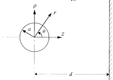
FIG. 1. Geometrical sketch for the diffusiophoretic motion of a spheri-which is unity if i equals m and zero otherwise; and v * is

cal particle perpendicular to a plane wall. the velocity of the interface, equal to zero for the fixed solid

boundary and U/V1r for a particle translating at velocity

U at a reference point and rotating at angular velocity V, _{lyte solute ( M} _Å _{1 ) in the direction normal to an infinite} where r is the position vector on the particle surface mea- _{plane wall located at a distance d from the particle center,} sured from the reference point. To obtain Eqs. [ 2.5 ] and _{as shown in Fig. 1. Here, ( r, f, z ) and ( r , u, f ) denote the} [ 2.6 ] , it has been assumed that the equilibrium concentration _{circular cylindrical and the spherical coordinates,} respec-of any species is related to its equilibrium potential energy _{tively, and the origin of coordinates is chosen at the particle} by the Boltzmann distribution. _{center. The concentration gradient of the solute far away} The modified chemical potentials in the outer region far _{from the particle,}Ç_n`_{, is a constant along the axial direction}

away from the particle approach the undisturbed values: _{( n}`_{is a linear function of z only ) . It is assumed that a}_ÉÇ_n`_É_/

n`( 0 ) ! 1 and L / a * ! 1, where L is the characteristic mmr m

0

m/kT ln n`m/F`m. [ 2.7 ] _{thickness of the particle-solute interaction layer ( which is}

approximately the molecular dimension of the solute ) and In Eq. [ 2.7 ] , F`m Å 0 for the case of nonionic

diffusio-a * is the smdiffusio-aller of diffusio-a diffusio-and d0 a . The interaction between

phoresis andÇ_F`_m_{Å 0}_z_m_eE`_{for the cases of ionic}

diffusio-the solute molecules and diffusio-the particle surface is described by phoresis ( in which E` is an induced electric field given by

the potential energy F( yn) , which decays to zero when

Eq. [ 4.1] ) and electrophoresis, where zm is the valence of

yn/ L@1. Our purpose is to determine the correction to Eq.

type-m ions. If there is no ‘‘osmotic’’ flow generated by the

[1.8 ] for the particle velocity due to the presence of the fixed solid boundary, one has the condition vr0 far from

plane wall. the particle.

Before determining the diffusiophoretic velocity for the Because there is no effective external field exerted beyond

particle, the modified chemical potential and velocity fields the outer edge of the particle – solute interaction layer, the

in the surrounding fluid must be solved. particle ( plus its adjacent diffuse layer of solute species ) is

force and torque free. With this constraint, one can calculate

3.1. Modified Chemical Potential Distribution

the particle velocities U and V after solving Eqs. [ 2.1] and

[ 2.2 ] for the modified chemical potentials and the fluid ve- The modified chemical potential energy m of the solute locity. For a spherical particle in an unbounded solution, the obeys Laplace’s equation ( Eq. [ 2.1] ) and is subject to the electrophoretic and diffusiophoretic velocities can be deter- following boundary conditions at the surfaces ( or, more pre-mined through the above procedure and the results are given cisely, at the outer edges of the thin particle-solute interac-by Eqs. [1.4 ] , [1.8 ] , and [1.9 ] . There is no rotational motion tion layers ) of the particle and the plane wall and far away of the isolated sphere due to the axial symmetry. from the particle according to Eqs. [ 2.4 ] and [ 2.7 ] ,

3. DIFFUSIOPHORESIS NORMAL TO A PLANE WALL _Ì_m

Ìr Å 0b

F

Ç 2 0 1 r2 Ì Ìr

S

r 2 Ì Ìr

DG

m at r Åa , IN A NONELECTROLYTE GRADIENT

In this section we consider the diffusiophoretic motion of

(5)

where Pn is the Legendre polynomial of order n and Tn

mÅ m0

/kT ln n` at z Åd , [ 3.1b ]

are the unknown coefficients to be determined. Note that a mr m0_/

kT ln n` as r r `and z£d . [ 3.1c ]

solution of m in the form given by Eqs. [ 3.4 ] – [ 3.6 ] immedi-ately satisfies boundary condition [ 3.1c ] .

In Eq. [ 3.1a ] , the relaxation coefficient

A brief conceptual description of the solution procedure to determine R ( v ) and Tnis given below to help the readers

bÅ( 1 /nPe ) K , [ 3.2 ] _{follow the mathematical development. At first, boundary} condition [ 3.1b ] is exactly satisfied on the plane wall by

with _{using a Hankel transform. This permits the unknown}

func-tion R ( v ) to be determined in terms of the coefficients Tn.

Then boundary condition [ 3.1a ] on the particle surface can

KÅ

*

`

0

[ exp (0F( yn) / kT )01] dyn, [ 3.3a ]

be satisfied by making use of the collocation method and the solution of the collocation matrix provides numerical nÅ( L * K2 )01

*

` 0

H

*

` 0 [ exp (0F( y*n) / kT )01] dy*n

J

2

dyn, _{values for the coefficients T} n.

Substitution of the solution m given by Eqs. [ 3.4 ] – [ 3.6 ] [ 3.3b ] into the boundary condition [ 3.1b ] and application of the Hankel transform on the variable r lead to a solution for PeÅ kT

hDL * Kn

`_{( 0 ) ,} _{[ 3.3c ]} _{R ( v ) in terms of the unknown coefficients T}

n. After the

substitution of this solution into Eq. [ 3.5 ] , the resulting chemical potential field is given by

and mÅm0 / kT ln n`/

∑

` n Å0 Tn[ B9n( r, z )0B9n( r, 2 d0z ) ] , L * ÅK01

*

` 0 yn[ exp (0F( yn) / kT )01] dyn. [ 3.3d ] [ 3.7 ] Here, D is the solute diffusion coefficient, Pe is the Peclet

number, and nPe accounts for the effect of convection on _{where the function B}₉

n( r, z ) is defined by Eq. [ A.12 ] in the

the solute distribution just outside the adsorption layer. The _{Appendix. Eq. [ 3.7 ] provides an exact solution for the} chem-concentration at the plane wall has been set equal to a

con-ical potential distribution and the unknown coefficients Tn

stant to allow a uniform solute gradient in the axial direction

must be determined from the remaining boundary condition far away from the particle.

[ 3.1a ] on the particle surface. Utilizing the relation Since the governing equation and boundary conditions are

linear, one can write the chemical potential distribution as

the superposition Ì Ìr Åsin u Ì Ìr/cos u Ì Ìz, [ 3.8 ] m Åm0 /kT ln n` /mw /ms. [ 3.4 ]

one can apply boundary condition [ 3.1a ] to [ 3.7 ] to yield Here, mwis a Fourier – Bessel integral solution of Laplace’s

equation in the cylindrical coordinates that represents the

_∑

`

n Å0 Tn

FS

2b r 01

D

a*n( r, z )/ b r g*n( r, z )

G

disturbance produced by the plane wall and is given by

ÅkTÉÇn `_É n`( 0 )

S

2b r 01

D

z at r Åa . [ 3.9 ] mw Å

*

` 0 vR ( v ) J0( vr ) evzd v, [ 3.5 ]

where J0 is the Bessel function of the first kind of order _{Here, the functions a}_*_n_{( r, z ) and g}_*_n_{( r, z ) are defined by} zero and R ( v ) is an unknown function of v. The last term _{Eqs. [ A.1] and [ A.2 ] .}

on the right-hand side of Eq. [ 3.4 ] , ms, is a solution of _{To satisfy the condition [ 3.9 ] exactly along the entire} Laplace’s equation in spherical coordinates representing the _{surface of the particle would require the solution of the entire} disturbance generated by the particle and is given by an _{infinite array of unknown coefficients T}_n_{. However, the} col-infinite series in harmonics, _{location technique ( 17 – 19 ) enforces the boundary condition} at a finite number of discrete points on the semicircular generating arc of the particle and truncates the infinite series msÅ

∑

` n Å0 Tnr 0 ( n /1 ) Pn( cos u ) , [ 3.6 ]

(6)

approximated by satisfying condition [ 3.1a ] at Nc discrete The stream function is linearly composed of two parts: points on its generating arc, the infinite series in Eq. [ 3.7 ]

is truncated after Ncterms, resulting in a system of Ncsimul- CÅCw /Cs. [ 3.14 ] taneous linear algebraic equations in the truncated form of

Eq. [ 3.9 ] . This matrix equation can be solved to yield the Here Cwis a solution of Eq. [ 3.10 ] in cylindrical coordinates

Nc unknown coefficients Tn required in the truncated form that represents the disturbance produced by the plane wall

of Eq. [ 3.7 ] for the chemical potential distribution. The and is given by a Fourier – Bessel integral, accuracy of the truncation technique can be improved to any

degree by taking a sufficiently large value of Nc. Naturally,

CwÅ

*

`

0

r J1( vr ) [ X ( v )/ zY ( v ) ] evz

d v, [ 3.15 ] as Nc r `the truncation error vanishes.

3.2. Fluid Velocity Distribution _{where J1}_{is the Bessel function of the first kind of order one}

and X ( v ) and Y ( v ) are unknown functions of v. The sec-With knowledge of the solution for the modified chemical

ond part of C, denoted by Cs, is a solution of Eq. [ 3.10 ] in potential distribution in the fluid phase, we can now proceed

spherical coordinates representing the disturbance generated to find the flow field. The velocity distribution for the fluid

by the particle and is given by outside the thin particle – solute interaction layer is governed

by the Stokes equations ( Eqs. [ 2.2 ] ) or the following

quasi-steady fourth-order differential equation for axisymmetric _Cs_Å

∑

` n Å2

( Bnr0n /1 /Dnr0n /3) G01 / 2n ( cos u ) , [ 3.16 ]

slow viscous flow,

where G01 / 2

n is the Gegenbauer polynomial of the first kind

E4 CÅE2

( E2

C )Å0, [ 3.10 ]

of order n and degree01/2; Bnand Dnare unknown constants.

Note that boundary condition [3.13c] is immediately satisfied where the Stokes stream function C is related to the velocity

by a solution of the form given by Eqs. [3.14] – [3.16]. components in cylindrical coordinates by

As was the case with the solution for the modified chemi-cal potential distribution, the determination of X ( v ) , Y ( v ) ,

£_rÅ 1

r

ÌC

Ìz , [ 3.11a ] Bnand Dnwill be undertaken by a two-step procedure. First,

boundary condition [ 3.13b ] is exactly satisfied on the plane wall by a Hankel transform; then, boundary condition

£_z_{Å 0} 1

r

ÌC

Ìr , [ 3.11b ] [ 3.13a ] is satisfied numerically at collocation points on the particle surface. Application of boundary condition [ 3.13b ] to Eqs. [ 3.14 ] – [ 3.16 ] using Eq. [ 3.11] leads to a solution and the operator E2

has the form

for X ( v ) and Y ( v ) in terms of the unknown coefficients

Bnand Dn. This solution is substituted back into Eq. [ 3.15 ] ,

E2_Å r Ì Ìr

S

1 r Ì Ìr

D

/ Ì2

Ìz2. [ 3.12 ] leading to a new expression for the stream function. Pre-sented below is the result for the velocity components, The boundary conditions for the velocity field, resulting

£_r Å

∑

` n Å2

[ Bnb*n( r, z )/Dnd*n( r, z ) ] , [ 3.17a ]

from Eq. [ 2.5 ] and the fact that the fluid is motionless far away from the particle, are

£_z_Å

∑

` n Å2 [ Bnbn9( r, z )/Dndn9( r, z ) ] , [ 3.17b ] vÅUez0 1 h n `_{( 0 ) L * K}_Ç_sm _{at r} _Å_{a , [ 3.13a ]}

where the functions b*n, d*n, bn9, dn9 are defined by Eqs.

vÅ0 at z Åd , [ 3.13b ]

[ A.4 ] – [ A.7 ] .

vr0 as r r `and z£ d , [ 3.13c ] _{The only boundary condition that remains to be satisfied} is that on the particle surface. Substituting Eq. [ 3.7 ] into where ez is the unit vector in the axial direction and U is Eq. [ 3.13a ] one obtains

the instantaneous diffusiophoretic velocity to be determined. There will be no rotation of the particle due to the axial

£_r_{Å 0} 1 hL * Kn `_{( 0 )} z ( r2 /z2 ) [

∑

` n Å0 Tnan9( r, z )0 r ] ,

symmetry. In Eq. [ 3.13a ] , Ç_{sm can be obtained from the}

chemical potential distribution given by Eq. [ 3.7 ] with

(7)

be solved for unknown coefficients Tn is constructed from £_zÅU/1 h L * Kn `_{( 0 )} r ( r2_/ z2 ) [

∑

` n Å0

Tnan9( r, z )0r ] , _{Eq. [ 3.9 ] , while that for B}

n and Dn is composed of Eqs.

[ 3.17 ] and [ 3.18 ] . The details of the collocation scheme [ 3.18b ] _{used for this work were given in Keh and Lien ( 1991 ) .} The numerical calculations were performed by using a DEC at rÅa . The definition of an9( r, z ) is given by Eq. [ A.3 ] . 3000 / 600 workstation.

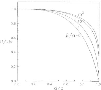
Here the first Nc coefficients Tn have been determined Numerical values of the wall-corrected reduced

diffusio-through the procedure given in the previous subsection. Ap- phoretic mobility for a sphere moving perpendicular to a plication of these boundary conditions to Eqs. [ 3.17 ] can be plane wall in a nonelectrolyte gradient for various values of accomplished by utilizing the collocation technique pre- the parameters b / a and a / d are presented in Table 1 and sented for the solution of the modified chemical potential depicted in Fig. 2. All of the results obtained under this field. At the particle surface, boundary conditions [ 3.18 ] are collocation scheme converge to at least five significant fig-applied at Nv discrete points ( values of u ) and the infinite ures. The accuracy of the truncation technique is principally series in Eqs. [ 3.17 ] are truncated after Nvterms. This gener- a function of the relative spacing a / d . For the difficult case ates a set of 2Nvlinear algebraic equations for the 2Nvun- of a / dÅ0.995, the number of collocation points NcÅ140 known coefficients Bn and Dn. The fluid velocity field is and NvÅ160 are sufficiently large to achieve this

conver-completely solved once these coefficients are determined. gence. As expected, the particle will move with the velocity that would exist in the absence of the wall, given by Eq.

3.3. Velocity of the Particle _{[1.8 ] , as a / d}_Å_{0. The diffusiophoretic velocity then steadily}

decreases as the particle approaches the wall ( with increas-The drag force exerted by the fluid on the spherical

bound-ing a / d ) , gobound-ing to zero at the limit. It can be seen that ary rÅa can be determined from ( 20 )

the retardation effect produced by the wall is a monotonic decreasing function of b / a . For the case of b / a Å 0, the

F Åhp

*

p 0 r3 sin3_u Ì Ìr

S

E2_C r2 sin2

u

D

rdu. [ 3.19 ] diffusiophoretic mobility of the sphere is identical to the prediction by ignoring the polarization effect of the diffuse layers ( 16, 17 ) .

Substitution of Eqs. [ 3.14 ] – [ 3.16 ] into the above integral

and application of the orthogonality properties of the Gegen- _{4. DIFFUSIOPHORESIS NORMAL TO A PLANE WALL} bauer polynomials result in the simple relation _{IN AN ELECTROLYTE GRADIENT}

F Å4phD2. [ 3.20 ] _{We now consider the axisymmetric diffusiophoretic} mo-tion of a colloidal sphere of radius a in a solumo-tion of symmet-This shows that only the coefficient D2 contributes to the

drag force on the particle.

Since the diffusiophoretic particle is freely suspended in TABLE 1

the fluid, the net force exerted by the fluid on the surface of The Normalized Diffusiophoretic Mobility of a Collodial Sphere Moving Perpendicular to a Plane Wall in a Nonelectrolyte Solute

the particle must vanish. From Eq. [ 3.20 ] , we have D2 Å

Gradient

0. The diffusiophoretic velocity U of the particle is to be obtained by satisfying this constraint. The normalized

parti-U/U0 cle velocity U / U0will be a function of the relaxation

param-eter b / a and the separation paramparam-eter a / d , where U0is the _a/d b/aÅ0.1 b/aÅ1.0 b/aÅ10 diffusiophoretic velocity of the particle in the absence of the

0 1 1 1

plane wall and is given by Eq. [1.8 ] . By the linearity of the

0.1 0.99941 0.99957 0.99972

problem, the same value of the normalized diffusiophoretic

0.2 0.99532 0.99655 0.99778

velocity is predicted for a given combination of b / a and _0.3 _0.98425 _0.98845 _0.99264

a / d whether the particle is approaching the plane wall or 0.4 0.96251 0.97269 0.98277

receding from it. 0.5 0.92564 0.94614 0.96636

0.6 0.86739 0.90437 0.94076

0.7 0.77800 0.83997 0.90133

3.4. Results and Discussion

0.8 0.64028 0.73827 0.83840

0.9 0.41854 0.56121 0.72453

The solution for the diffusiophoretic motion of a colloidal

0.95 0.25031 0.40497 0.61603

sphere normal to a plane wall in a nonelectrolyte gradient,

0.99 0.06144 0.16596 0.41482

using the boundary collocation technique, will be presented

0.995 0.03188 0.10876 0.35021

(8)

sidered a linear combination of two effects: ( 1 ) ‘‘chemi-phoresis’’ due to the nonuniform adsorption of counterions over the surface of the particle, which is analogous to diffusiophoresis in nonelectrolytes considered in the previ-ous section; ( 2 ) ‘‘electrophoresis’’ due to the macroscopic electric field generated by the gradient of electrolyte concen-tration given by Eq. [ 4.1] . In Eq. [1.3 ] for the diffusiopho-retic velocity of a particle with an unpolarized double layer, the first term in the brackets results from the contribution of electrophoresis, while the other term represents the chemi-phoretic contribution.

4.1. Modified Chemical Potential Distributions

The modified chemical potentials ( also termed electro-chemical potentials ( 21 ) ) of the ions outside the double layers satisfy Laplace’s equation [ 2.1] and are subject to the boundary conditions ( according to Eqs. [ 2.4 ] and [ 2.7 ] )

FIG. 2. Plots of the normalized diffusiophoretic mobility of a spherical particle in the direction perpendicular to a plane wall versus the separation

parameter for various values of the relaxation parameter b / a . Ìmm

Ìr Å 0

∑

2 i Å1 bmi

F

Ç 2 0 1 r2 Ì Ìr

S

r 2 Ì Ìr

DG

mi at r Åa , [ 4.2a ] rically charged, binary electrolyte ( MÅ2 ) toward an infinite

plane wall whose distance from the particle is d . The

concen-mmÅm

0

m/kT ln n` /zmeF`e at z Åd , [ 4.2b ]

tration gradient Ç_n` _{of the electrolyte is a constant along}

the axial direction ( n`1 Ån`2 Ån`, where subscripts 1 and m_mrm0_m/kT ln n` /z_meF`_e as r r `and z£ d , 2 refer to the anion and cation, respectively ) . Again we

[ 4.2c ] assume aÉÇn`É/ n`( 0 )! 1. The thickness of the electrical

double layer ( similar to the particle – solute interaction layer

in the previous section ) , which is characterized by the Debye where mÅ1 or 2. Analytical expressions of the relaxation length k01

, is assumed to be much smaller than the radius coefficients bmifor a symmetric electrolyte can be obtained

of the particle and the gap width between the particle and as ( 9, 13 ) the plane wall. However, the effect of polarization of the

diffuse layer will be taken into account. The interaction

be-b11Å 1

k

F

4

S

1/ 3 f1

Z2

D

exp ( zU ) sinh zU tween the diffuse ions and the charged surfaces of the particle

and the wall is dominated by the electrical energies Fm Å

zmeFe, where zmis the valence of ions m ( mÅ1 or 2;0z1

012 f1

Z2 ( zU /ln cosh zU )

G

, [ 4.3a ]

Åz2 ÅZ ) and Fe is the electrical potential. The objective

here is to determine the correction to Eq. [1.9 ] for the particle due to the presence of the wall.

b12Å01

k

S

12 f1

Z2

D

ln cosh zU , [ 4.3b ] Since n`is not uniform, it is required that the total fluxes

of cations and anions are equal in order to have no current arising from the diffusive fluxes of the solute ions in an

b21Å01

k

S

12 f2

Z2

D

ln cosh zU , [ 4.3c ] electrically neutral solution. So an electric field arises

spon-taneously due to the difference in mobilities of the cation

and the anion ( 6 ) , _b22_Å 1

k

F

04

S

1/ 3 f2 Z2

D

exp (0zU ) sinh zU E` Å 0ÇF`e Å kT Ze

S

D20D1 D2/D1

D

Ç _{ln n}`_. _{[ 4.1]} _/12 f2 Z2 ( zU 0ln cosh zU )

G

, [ 4.3d ] where zV Å Zez / 4kT and fm Å e( kT )2/ 6phe2Dm; z is the

Because all the governing equations and boundary

(9)

wall must be a conducting one to allow the electrolyte con- section can be used. The infinite series in solution [ 4.4 ] and boundary conditions [ 4.5 ] are truncated after Ncterms and centration and the electrical potential to be constant on it.

Similarly to the analysis to obtain Eq. [ 3.7 ] in the previous the truncated form of Eqs. [ 4.5 ] is applied at Nc discrete points ( values of u ) along the particle surface. This generates section, the solution for the modified chemical potentials

that satisfies the boundary condition [ 4.2b ] at the plane wall a system of 2Nclinear algebraic equations for 2Ncunknown coefficients T1nand T2n. Once these coefficients are deter-and the far-field condition [ 4.2c ] is given by

mined, the solution for the electrochemical potential fields is completely known. mmÅm0m/kT ln n` 0 zm Z

S

D20D1 D2/D1

D

kTÉÇ_n`É n`( 0 ) z

4.2. Fluid Velocity Distribution

Having obtained the modified chemical potential

distribu-/

∑

` n Å0

Tmn[ B9n( r, z )0B9n( r, z ) ] , [ 4.4 ] _{tions in the fluid phase, we can now take up the solution of}

the flow field. The velocity distribution for the fluid outside the thin double layers is governed by the same equation as where mÅ1 or 2 and T1nand T2nare unknown coefficients _{Eq. [ 3.10 ] and obeys boundary condition [ 3.13b ] at the} to be determined by using the boundary condition [ 4.2a ] on _{plane wall and condition [ 3.13c ] at infinity. The boundary} the particle surface. In addition to the contribution of the _{condition on the particle surface becomes ( 9, 13 )}

undisturbed solute distribution to mm, a contribution due to

the induced electric field given by Eq. [ 4.1] is also included

in Eq. [ 4.4 ] . Substituting Eq. [ 4.4 ] into Eq. [ 4.2a ] with the vÅUez0

e 2ph

kT

(Ze )2[ ( zU /ln cosh zU )Çsm1 help of Eq. [ 3.8 ] yields

/(0zU / ln cosh zU )Ç_sm2] _{at r} _Å_{a .} _{[ 4.6 ]}

∑

` n Å0 T1n

FS

2b11 r 01

D

a*n( r, z )/ b11

r g*n( r, z )

G

The velocity components£_r_and£_z_{for the fluid flow}

satis-fying Eqs. [ 3.10 ] , [ 3.13b ] , and [ 3.13c ] can be expressed by Eqs. [ 3.17 ] , and the unknown coefficients Bn and Dn

/

∑

` n Å0

T2n b12

1 2

∑

` n Å0 ( T1n/T2n) an9( r, z )0 kTÉÇn`É n`( 0 ) r

GJ

, at r Å a , where a*n( r, z ) and g*n( r, z ) have been defined

by Eqs. [ A.1] and [ A.2 ] .

(10)

TABLE 2

The Normalized Diffusiophoretic Mobility of a Dielectric Sphere Moving Perpendicular to a Plane Wall in a Concentration Gradient of Symmetric Electrolytes for the Case f1Å 0.2 and ka Å 100

U/U0 D20D1Å0 (D20D1)/(D2/D1)Å 00.2 ze/kT a/d ZÅ1 ZÅ2 ZÅ3 ZÅ1 ZÅ2 ZÅ3 2 0.2 0.99542 0.99575 0.99649 0.99900 0.99629 0.99718 0.4 0.96340 0.96616 0.97224 0.99363 0.97066 0.97803 0.6 0.87088 0.88114 0.90332 0.98667 0.89819 0.92487 0.8 0.65020 0.67774 0.73635 0.97061 0.72431 0.79431 0.9 0.43157 0.46989 0.55377 0.86353 0.53351 0.63469 0.95 0.26107 0.29872 0.38678 0.64904 0.35809 0.46680 0.99 0.06415 0.08142 0.13325 0.20075 0.10512 0.17289 0.995 0.03314 0.04341 0.07836 0.10741 0.05692 0.10345 0.999 0.0068 0.0093 0.0206 0.0228 0.0124 0.0279 5 0.2 0.99628 1.00286 0.99401 0.99697 0.94469 0.99440 0.4 0.97053 1.02471 0.95170 0.97634 0.54463 0.95489 0.6 0.89716 1.09373 0.82756 0.91883 00.65639 0.83917 0.8 0.72012 1.24760 0.53172 0.77856 03.45318 0.56328 0.9 0.53023 1.32572 0.25688 0.61143 05.66735 0.30540 0.95 0.36136 1.27559 0.06941 0.44068 06.56694 0.12688 0.99 0.11668 0.89325 00.09369 0.15405 05.35463 00.03745 0.995 0.06661 0.71943 00.10654 0.08961 04.41782 00.05452 0.999 0.0164 0.4096 00.1000 0.0226 02.5812 00.0582 8 0.2 0.99891 0.99445 0.99497 1.00328 0.99465 0.99497 0.4 0.99215 0.95532 0.95957 1.02829 0.95696 0.95962 0.6 0.97530 0.84076 0.85622 1.10736 0.84673 0.85639 0.8 0.92796 0.56756 0.60962 1.28087 0.58380 0.61009 0.9 0.84043 0.31182 0.37668 1.35480 0.33682 0.37738 0.95 0.71257 0.13417 0.21138 1.26913 0.16381 0.21218 0.99 0.39361 00.03137 0.04536 0.78093 00.00210 0.04611 0.995 0.28754 00.04945 0.02208 0.58261 00.02173 0.02277 0.999 0.1295 00.0554 0.0035 0.2693 00.0331 0.0040 UÅUc /Ue [ 4.8 ] at r Å a , where an9( r, z ) has been defined by Eq. [ A.3 ] .

To use the collocation technique, the infinite series in Eqs.

where Uc

and Ue

denote the corresponding chemiphoretic [ 3.17 ] are truncated after Nvterms and the boundary

condi-and electrophoretic velocities, respectively. Uc

can be deter-tions [ 4.7 ] ( in which the coefficients T1nand T2nare

deter-mined from the same procedure by setting D1ÅD2in Eq. mined through the procedure given in the previous

subsec-[ 4.4 ] for mm. Uecan also be determined similarly by taking

tion ) are applied at Nv discrete points along the particle

the second term on the right-hand side of Eq. [ 4.4 ] as a surface. The resulting system of 2Nvlinear algebraic

equa-constant. tions can be solved to yield the 2Nv unknown coefficients

Bn and Dn. The velocity distribution is completely

deter-4.4. Results and Discussion

mined once these coefficients are obtained.

In this subsection, we present the solution for the

diffus-4.3. Velocity of the Particle

iophoretic motion of a dielectric sphere normal to a con-ducting plane in a constant gradient of a symmetric elec-Because the diffusiophoretic particle is freely suspended

in the fluid, the drag force exerted on the particle, which trolyte. To use the boundary collocation technique, Eqs. [ 4.5 ] are applied to solve the coefficients T1nand T2nfor is still given by Eq. [ 3.20 ] , vanishes. By satisfying this

requirement, the particle velocity is determined. Due to the m1and m2, and Eqs. [ 3.17 ] and [ 4.7 ] are applied to solve coefficients Bnand Dnfor the velocity field. The

diffusio-linearity of the diffusiophoretic problem, the particle

(11)

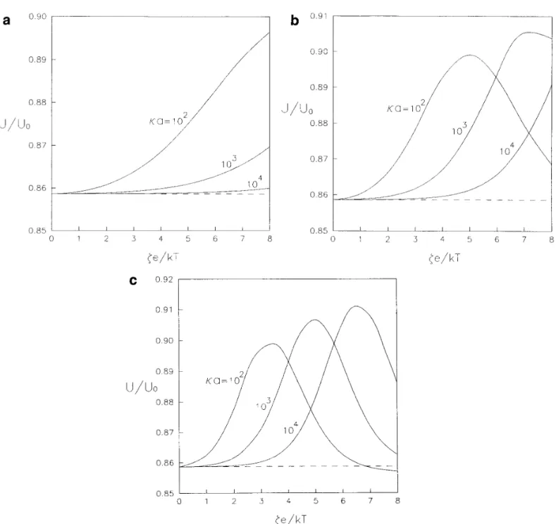
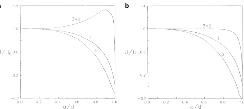
FIG. 3. Plots of the normalized diffusiophoretic mobility of a spherical particle in the direction perpendicular to a plane wall versus the separation parameter with f1Å0.2 and kaÅ100: ( a ) D20D1Å0 and ze / kTÅ5; ( b ) ( D20D1) / ( D2/D1)Å 00.2 and ze / kTÅ 05.

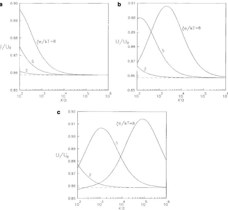
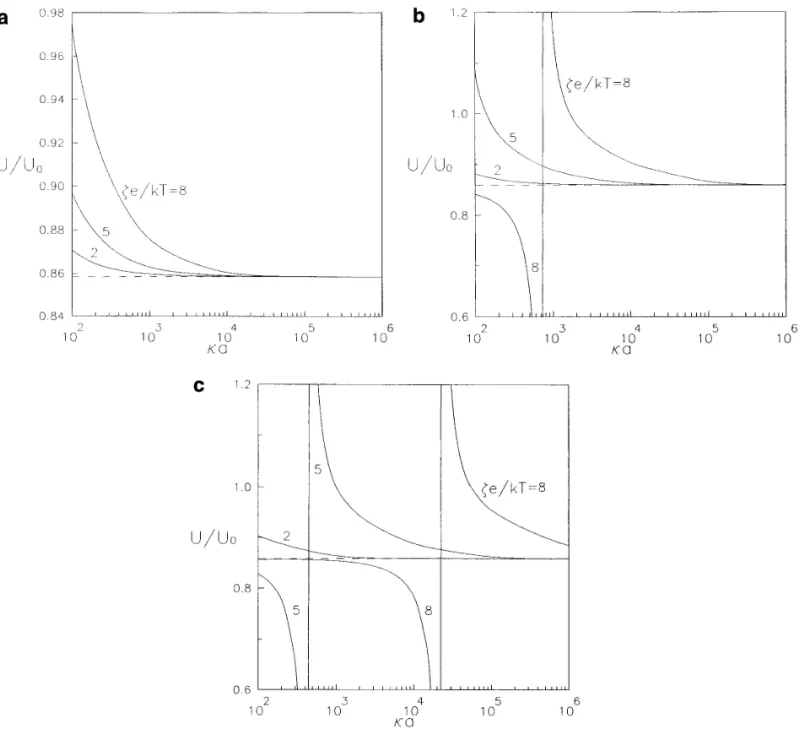
various values of ( D20D1) / ( D2/D1) , f1, Z , ze / kT , ka , plotted versus ka in the range from 102to 106 for cases of ( D20D1) / ( D2/D1)Å0 and00.2, respectively ( with and a / d . Part of the numerical results of the normalized

diffusiophoretic mobility as a function of the separation a / d Å0.6 ) . It is evident that, as ka becomes very large, the diffusiophoretic mobility of the sphere will approach parameter a / d are presented in Table 2 and depicted in

Fig. 3 ( with f1Å0.2, kaÅ100, ZÅ1, 2, and 3 ) . All the the value calculated by ignoring the polarization effect of the double layers ( shown by a dashed line in each figure ) . data in Table 2 are at least convergent to the digits as

shown. Only the results at positive zeta potentials are From Figs. 4a and 5a for the case Z Å 1, the boundary effect is weakened steadily ( the value of U / U0is getting displayed when D1 Å D2 since the induced electric field

given by Eq. [ 4.1] vanishes and the particle velocity, close to unity ) as ka becomes small gradually. A novel result is that, as shown in Figs. 4b, 4c, 5b, and 5c for Z which is due to the chemiphoretic effect only, is an even

function of zeta potential. It can be seen that the diffusio- Å2 and ZÅ3, there can be a maximum and a minimum of the normalized particle mobility occurring at some ka phoretic mobility of the particle is not necessarily a

mono-tonic function of a / d . For some cases, the particle will for the representative cases of ze / kT Å 05, 5, and 8. If the particle is charged more highly or the counterions reverse the direction of diffusiophoresis and the

magni-tude of its normalized velocity can be dramatically varied have a larger magnitude of valence, the locations of these maximal boundary effects will shift toward larger ka ; that when the separation distance is decreased. In general, no

theoretical rule could appropriately predict the boundary means larger values of ka are required to make the as-sumption of kar `valid. Because the direction of diffusi-effect on diffusiophoresis. The fact that both the

chemi-phoretic and the electrochemi-phoretic effects ( which react dif- ophoresis of an isolated particle can reverse with the varia-tion of ze / kT or ka ( 11 – 13 ) , these extremes arise at com-ferently to the neighboring wall ) contribute to the

parti-cles’ movement is responsible for this complexity. Al- binations of ze / kT and ka in which the magnitude of U0 is very small.

though it is difficult to obtain convergent results of the particle velocity for situations of very small separation

distance ( a / dú0.999 ) , both the physical reasoning and 5. ELECTROPHORESIS NORMAL TO A PLANE WALL

the numerical tendency indicate that U / U0r 0 as a / d r

Considered in this section is the axisymmetric electropho-1. Note that the electrolytes associated with ( D2 0 D1) /

retic motion of a charged particle of radius a toward an ( D2/ D1) Å0 and 00.2 in Table 2 and Fig. 3 are very

infinite plane wall whose distance from the particle is d . close to the aqueous solutions of KCl and NaCl,

respec-The applied electric field is uniform and equal to E`ez. The

tively.

In Figs. 4 and 5, the normalized diffusiophoretic mobil- bulk concentrations of all ions n`mbeyond the electrical

dou-ble layers are constant. It is assumed that ka@ 1 and k( d ity of a particle moving perpendicular to a plane wall is

(12)

FIG. 4. Plots of the normalized diffusiophoretic mobility of a spherical particle in the direction perpendicular to a plane wall versus the ratio of the particle radius to the Debye length with a / dÅ0.6 and f1Åf2Å0.2 ( D20D1Å0 ) : ( a ) ZÅ1; ( b ) ZÅ2; ( c ) ZÅ3.

0a )@1, but the effect of double layer relaxation is incorpo- boundary conditions [ 4.2 ] ( with F`e Å 0E`z ) . Similar

rated. The potential energy Fmof ionic species m is equal to Eqs. [ 3.7 ] and [ 4.4 ] , the solution for the

electrochemi-to zmeFe. For simplicity, only one symmetric electrolyte in cal potentials that satisfies Eqs. [ 4.2b ] and [ 4.2c ] can be

expressed as the liquid phase ( M Å 2; 0z1 Å z2 Å Z ; n`1 Å n`2 Å n`,

where subscripts 1 and 2 denote anion and cation, respec-tively ) will be considered. Now the object is to obtain the _m

mÅm

0

m /kT ln n` 0zmeE`z

correction to Eq. [1.4 ] for the particle due to the presence

of the wall. _/

_∑

`

n Å0

Tmn[ B9n( r, z )0B9n( r, 2 d 0z ) ] , [ 5.1]

5.1. Modified Chemical Potential Distributions

Outside the double layers, the electrochemical poten- where mÅ1 or 2 and T1nand T2nare unknown coefficients to be determined from the boundary condition [ 4.2a ] . tials of the ions satisfy Laplace’s equation [ 2.1] and the

(13)

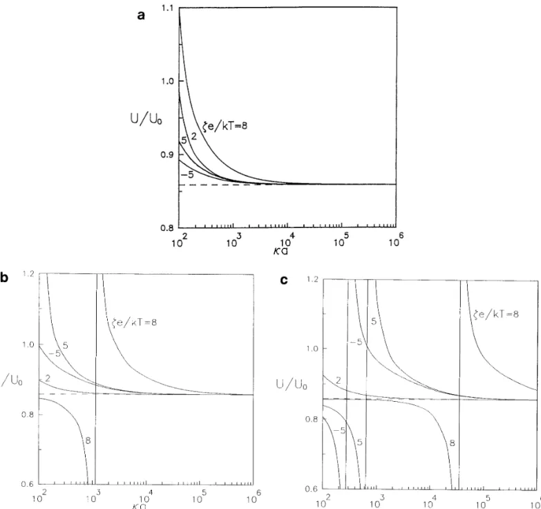
FIG. 5. Plots of the normalized diffusiophoretic mobility of a spherical particle in the direction perpendicular to a plane wall versus the ratio of the particle radius to the Debye length with a / dÅ0.6, ( D20D1) / ( D2/D1)Å 00.2, and f1Å0.2: ( a ) ZÅ1; ( b ) ZÅ2; ( c ) ZÅ3.

Substituting Eq. [ 5.1] into Eq. [ 4.2a ] with the help of Eq.

∑

` n Å0 T1n b21 r [ 2a*n( r, z )/ g*n( r, z ) ] [ 3.8 ] results in /

∑

` n Å0 T2n

FS

2b22 r 01

D

a*n( r, z )/ b22 r g*n( r, z )

G

∑

` n Å0 T1n

FS

2b11 r 01

D

a*n( r, z )/ b11 r g*n( r, z )

G

ÅZeE`

S

0102b21 r / 2b22 r

D

z , [ 5.2b ] /

∑

` n Å0 T2n b12 r [ 2a*n( r, z )/g*n( r, z ) ]

at rÅ a . As described in the previous sections, we can ÅZeE`

S

10 2b11

r /

2b12

r

D

z , [ 5.2a ]

use the collocation technique to solve the first Nc sets of the coefficients T1nand T2n.

(14)

TABLE 3 £_zÅU/ ez 4ph 1 Ze r ( r2_/ z2 )

The Normalized Electrophoretic Mobility of a Dielectric Sphere Moving Perpendicular to a Plane Wall in a Solution of Symmetric Electrolytes for the Case f1Å f2Å 0.2 and ka Å 100

1

F

∑

` n Å0 ( T1n0T2n) an9( r, z )0 2ZeE`r / kT Zez U/U0 ze/kT a/d ZÅ1 ZÅ2 ZÅ3 1ln cosh

S

Zez 4kT

D

∑

` n Å0 ( T1n/T2n) an9( r, z )

G

, [ 5.3b ] 2 0.2 0.99511 0.99528 0.99565 0.4 0.96076 0.96224 0.96529

0.6 0.86075 0.86633 0.87748 at rÅ a . The coefficients Bn and Dn can be solved by the

0.8 0.62218 0.63725 0.66684 _{substitution of the truncated form of Eqs. [ 3.17 ] into Eqs.} 0.9 0.39379 0.41460 0.45672 _{[ 5.3 ] using the collocation technique presented in the}

previ-0.95 0.22716 0.24713 0.29083

ous sections.

0.99 0.05222 0.06084 0.08574

0.995 0.02666 0.03169 0.04829

0.999 0.0054 0.0066 0.0119 _{5.3. Velocity of the Particle}

5 0.2 0.99557 0.99639 0.99557

0.4 0.96460 0.97135 0.96454 Similar to the cases of diffusiophoresis considered in the 0.6 0.87502 0.89916 0.87433 _{previous sections, the electrophoretic particle is freely}

sus-0.8 0.66040 0.72497 0.65886

pended in the fluid, and the drag force exerted on the particle,

0.9 0.44731 0.54830 0.45240

which is expressed by Eq. [ 3.20 ] , equals zero. The

electro-0.95 0.28047 0.40387 0.30114

phoretic velocity of the particle can be determined by

satis-0.99 0.07873 0.19900 0.13336

0.995 0.04327 0.14864 0.10354 fying this constraint. This particle velocity is the same as 0.999 0.0100 0.0774 0.0687 _{the electrophoretic velocity U}e

obtained in the previous

sec-8 0.2 0.99630 0.99538 0.99500

tion with the substitution of Eq. [ 4.1] .

0.4 0.97057 0.96295 0.95980

0.6 0.89645 0.86854 0.85707

0.8 0.71721 0.64315 0.61194 5.4. Results and Discussion

0.9 0.53339 0.42831 0.38026

0.95 0.38067 0.27270 0.21565 The solution for the electrophoresis of a charged sphere 0.99 0.16313 0.10610 0.04967 _{normal to a conducting plane in a symmetric electrolyte} 0.995 0.11205 0.07869 0.02613 _{will be presented in this subsection. To use the collocation}

0.999 0.0464 0.0496 0.0063

technique, Eqs. [ 5.2 ] are applied to solve the coefficients

T1n and T2n for m1 and m2, and Eqs. [ 3.17 ] and [ 5.3 ] are applied to solve Bnand Dnfor the flow field. The

electropho-retic velocity of the particle has been calculated for various

5.2. Fluid Velocity Distribution

values of f1, f2, Z , ze / kT , ka , and a / d . Part of the numerical results of the normalized electrophoretic mobility as a func-Same as the case of diffusiophoresis considered in the

tion of a / d are listed in Table 3. It can be seen that the previous section, the velocity distribution for the fluid

out-electrophoretic velocity of the particle is a monotonic de-side the double layers is governed by Eqs. [ 3.10 ] , [ 4.6 ] ,

creasing function of a / d and vanishes as a / dÅ1. [ 3.13b ] , and [ 3.13c ] . The solution for the velocity

compo-Figure 6 is drawn to show the effect of the plane wall on nents£_r_and£_z_{that satisfies boundary condition [ 3.13b ] and}

the electrophoretic sphere versus the particle’s zeta potential [ 3.13c ] is still given by Eqs. [ 3.17 ] , and the coefficients

for three cases of ka when the separation parameter a / d is

Bn and Dn are to be determined by using condition [ 4.6 ] .

kept constant. When Z Å 1, as illustrated in Fig. 6a, the Substituting Eq. [ 5.1] into Eq. [ 4.6 ] , one obtains

normalized electrophoretic mobility of the particle is a monotonic increasing function of the nondimensional zeta potential ze / kT ranging from 0 to 8. Also, the value of

£_rÅ 0 ez 4ph 1 Ze z ( r2 /z2

) _{U / U}₀_{is larger with smaller ka . However, when Z}_Å_{2 or 3} as shown in Figs. 6b and 6c, a maximum of U / U0exists for

1

F

∑

` n Å0

( T1n0T2n) an9( r, z )02ZeE`r/

kT

Zez some cases. When ka increases, the maximum occurs at a

larger zeta potential. Note that these maxima for the cases with ZÅ3 take place at smaller zeta potentials than those with ZÅ2. 1ln cosh

S

Zez 4kT

D

∑

` n Å0 ( T1n/T2n) an9( r, z )

G

, [ 5.3a ]

(15)

FIG. 6. Plots of the normalized electrophoretic mobility of a spherical particle in the direction perpendicular to a plane wall versus the dimensionless zeta potential with a / dÅ0.6 and f1Åf2Å0.2: ( a ) ZÅ1; ( b ) ZÅ2; ( c ) ZÅ3.

particle is plotted versus ka for three cases of ze / kT with 6. SUMMARY

a / dÅ 0.6. It is shown that the electrophoretic mobility of

the particle will approach the value calculated in the limit Three problems of similar physical and mathematical structures are studied in this work: the diffusiophoresis of a of Eq. [1.7 ] ( indicated by a dashed line ) for each case as

long as the value of ka approaches infinity. From Fig. 7a sphere normal to a plane in a nonelectrolyte solute gradient, the diffusiophoresis of a sphere normal to a plane in an for the case ZÅ1, the boundary effect is weakened steadily

as ka becomes small gradually. However, as shown in Figs. electrolyte solute gradient, and the electrophoresis of a sphere normal to a plane in an external electric field. Al-7b and 7c for Z Å 2 and 3 respectively, there can be a

maximum of U / U0at some ka for the representative cases though the region of the interaction between the solute spe-cies and the solid surfaces is taken to be small relative to of ze / kTÅ5 and 8. This observation can also be predicted

from Figs. 6b and 6c. If the particle is charged more highly the particle dimension and to the spacing between the parti-cle and the wall, the assumptions allow for polarization of or the counterions have a larger magnitude of valence, the

(16)

devel-FIG. 7. Plots of the normalized electrophoretic mobility of a spherical particle in the direction perpendicular to a plane wall versus the ratio of the particle radius to the Debye length with a / dÅ0.6 and f1Åf2Å0.2: ( a ) ZÅ1; ( b ) ZÅ2; ( c ) ZÅ3.

oped for treating the electrokinetic equations in the limit of the diffuse layer (or the value of b/a) is, the weaker the boundary effect on the diffusiophoresis is. For the case of thin double layer ( 4, 8 ) is used to obtain the equations of

conservation and the boundary conditions in the ‘‘outer’’ diffusiophoresis in an electrolyte gradient, the interaction be-tween the particle and the wall is a complicated function of region applicable to the problems.

A semianalytical procedure with the boundary collocation the properties of the particle and ions, and it no longer varies monotonically with the extent of separation for some situations. technique has been used to solve the modified chemical

poten-tial energy field and the velocity field in the fluid phase. The For the case of electrophoresis, the particle mobility decreases monotonically with the decrease in the separation distance be-migration velocity of the particle perpendicular to the plane

wall is calculated for various cases. For the case of diffusio- tween the particle and the wall, but it is not a simple function of the particle’s and ions’ properties. No general rule can make phoresis in a nonelectrolyte gradient, the particle mobility

de-creases monotonically as the particle approaches the wall and an adequate prediction for such complicated phenomena pres-ent in electrophoresis and ionic diffusiophoresis.

(17)

APPENDIX /[ n ( 2n /3 ) z0n ( 2n 01 ) r02

z3 For the purpose of conciseness the definitions of some _/_nr02

z ( r2_/ z2 ) ]r 1 ( r2 /z2 )( n /4 ) / 2Pn 01

F

z ( r2 /z2 )1 / 2

G

Pnis the Legendre polynomial of order n and G01 / 2n is the

02 ( n/1 ) ( d0 z ) B9n /1( r, 2 d0z ) , [ A.6 ]

Gegenbauer polynomial of the first kind of order n and de-gree01 / 2.

dn9( r, z )Å D9n( r, z )0D9n( r, 2 d0z )

/2 ( n02 ) ( d 0z ) B9n 01( r, 2 d0z ) _{ACKNOWLEDGMENT}

02 ( 2n 03 ) d ( d0z ) B9n( r, 2 d0z ) , [ A.7 ] _{This research was supported by the National Science Council of the}

Republic of China under Grant NSC83-0402-E002-067. where REFERENCES An( r, z )Å nz2 0 ( n/1 ) r2 r( r2 /z2 )( n /3 ) / 2Pn

F

z ( r2 /z2

)1 / 2

G

_{1. Anderson, J. L., Annu. Rev. Fluid Mech. 21, 61 ( 1989 ) .} 2. Henry, D. C., Proc. Roy. Soc. London A 133, 106 ( 1931 ) . 3. Morrison, F. A., J. Colloid Interface Sci. 34, 210 ( 1970 ) .

4. Dukhin, S. S., and Derjaguin, B. V., in ‘‘Surface and Colloid Science’’

0 nz r( r2 /z2 )( n /2 ) / 2Pn 01

F

z ( r2 /z2

)1 / 2

G

, [ A.8 ] ( E. Matijevic, Ed.) , Vol. 7, Wiley, New York, 1974.

5. Anderdon, J. L., Lowell, M. E., and Prieve, D. C., J. Fluid Mech. 117, 107 ( 1982 ) .

6. Prieve, D. C., Anderson, J. L., Ebel, J. P., and Lowell, M. E., J. Fluid Cn( r, z )Å[0( n/1 ) ( r2/z2)0n r 02 z2 ( r2_/ z2 ) Mech. 148, 247 ( 1984 ) .

7. O’Brien, R. W., and White, L. R., J. Chem. Soc. Faraday Trans. II /( n /1 ) ( n /3 ) r2

0 2n ( n/2 ) z2

74, 1607 ( 1978 ) .

8. O’Brien, R. W., J. Colloid Interface Sci. 92, 204 ( 1983 ) . /n2 r02 z4 ]r 1 ( r2_/ z2 )( n /5 ) / 2Pn

F

z ( r2_/ z2

)1 / 2

G

9. Chen, S. B., and Keh, H. J., J. Fluid Mech. 238, 251 ( 1992 ) . 10. Anderdon, J. L., and Prieve, D. C., Langmuir 7, 403 ( 1991 ) .

(18)

11. Prieve, D. C., and Roman, R., J. Chem. Soc. Faraday Trans. II 83, 17. Keh, H. J., and Lien, L. C., J. Fluid Mech. 224, 305 ( 1991 ) . 18. Gluckman, M. J., Pfeffer, R., and Weinbaum, S., J. Fluid Mech. 50, 1287 ( 1987 ) .

12. Pawar, Y., Solomentsev, Y. E., and Anderson, J. L., J. Colloid Inter- 705 ( 1971 ) .

19. Dagan, Z., Weinbaum, S., and Pfeffer, R., J. Fluid Mech. 117, 143 face Sci. 155, 488 ( 1993 ) .

13. Keh, H. J., and Chen, S. B., Langmuir 9, 1142 ( 1993 ) . ( 1982 ) .

20. Happel, J., and Brenner, H., ‘‘Low Reynolds Number Hydrodynam-14. Morrison, F. A., and Stukel, J. J., J. Colloid Interface Sci. 33, 88 (1970).

15. Keh, H. J., and Anderson, J. L., J. Fluid Mech. 153, 417 ( 1985 ) . ics,’’ Nijhoff, The Netherlands, 1983.

21. Ohshima, H., Healy, T. W., and White, L. R., J. Chem. Soc. Faraday 16. Keh, H. J., and Lien, L. C., J. Chinese Inst. Chem. Engrs. 20, 283