國
立 交 通 大 學
電子工程學系電子研究所碩士班
碩 士 論 文
H.264/AVC及SVC熵解碼器之分析與設計
Analysis and Design of Entropy Decoder for
H.264/AVC and Scalable Extension
研 究 生: 廖元歆
指導教授: 張添烜 教授
H.264/AVC及SVC熵解碼器之分析與設計
Analysis and Design of Entropy Decoder for
H.264/AVC and Scalable Extension
研 究 生: 廖元歆 Student:Yuan-Hsin Liao
指導教授: 張添烜博士 Advisor:Dr. Tian-Sheuan Chang
國 立 交 通 大 學
電子工程學系電子研究所碩士班
碩 士 論 文
A Thesis
Submitted to Department of Electronics Engineering & Institute of Electronics College of Electrical and Computer Engineering
National Chiao Tung University in Partial Fulfillment of the Requirements
for the Degree of Master of Science in
Electronics Engineering August 2010
Hsinchu, Taiwan, Republic of China
H.264/AVC 及 SVC 熵解碼器之分析與設計
研究生:廖元歆 指導教授:張添烜博士
國立交通大學
電子工程學系電子研究所碩士班
摘 要
近年來,由於 H.264/AVC 較以前的視訊標準有更佳的編碼效率,至今已被 廣泛使用在視訊應用系統中。要想實現高解析度畫面即時解碼,熵解碼器的效能 需求非常的高。因此,我們需要設計一個高效能的積體電路來加速熵解碼器的解 碼速度。 本篇研究提出一個適用於 H.264/AVC 以及 SVC 的高產量熵解碼器硬體設 計。首先,我們提出一個延遲均衡的雙符號內容適應性變動長度解碼器,並將解 碼程序中多餘的解碼步驟省略以加速解碼的進行。工作頻率相較於傳統的設計可 提高21%,而整體產量相較於我們之前的設計可提升 28.2%。接著,針對 H.264/AVC 的另一種亂度編碼,我們提出一個以混合式記憶體為架構之高產量內容適應性二 元算數解碼器。在整個解碼架構中,我們將語法單元剖析及其解碼進行合併,並 提出以混合式記憶體為架構的雙符號平行解碼技術來加速解碼速度。更進一步 的,我們利用一個有效率的預測機制以及透過數學上的轉換來提升解碼效能。 基於聯華電子 90 奈米製程,我們的內容適應性變動長度解碼器的最高工作 頻率可達390 MHz,13.88k 個邏輯閘。而我們的內容適應性二元算數解碼器的 最高工作頻率可達 264 MHz,42.37k 個邏輯閘。我們的解碼器在節省了 48.6%的硬體成本下的產量為每秒 451.4 百萬個符號,高於其他已被發表的設計。此外,
我們將硬體設計拓展到SVC。在工作頻率 135 MHz 下,我們所提出的熵解碼器可
支援 3 層解析度,最高 1920x1080、三層播放頻率、最高每秒 60 張畫面、以及
Analysis and Design of Entropy Decoder for
H.264/AVC and Scalable Extension
Student: Yuan-Hsin Liao Advisor: Dr. Tian-Sheuan Chang
Department of Electronics Engineering & Institute of Electronics
National Chiao-Tung University
Abstract
In recent years, the state-of-the-art video coding standard H.264/AVC which provides better compression efficiency for video images than the earlier standards has been widely adopted in current video application system. To satisfy the heavy performance requirement on real-time H.264/AVC decoding systems especially for large-scale video sequences, VLSI implementation of the entropy decoder is necessary since it dominates the overall decoder system performance.
In this thesis, we propose a high-throughput and fully hardwired entropy decoder for H.264/AVC and its scalable extension. First, we present a delay balanced two-level CAVLC decoder with 21% shorter critical path delay in comparison to traditional two-level decoder. Furthermore, a skipping mechanism is adopted to remove unnecessary decoding processes. The overall CAVLC throughput is 28.2% better than our previous design. Second, for the CABAC decoder, we propose a high throughput CABAC decoding design which combines SE parsing and decoding with a new hybrid memory two-symbol parallel decoding technique to accelerate the decoding speed while reducing the hardware cost. Further speedup is achieved to
avoid stalls for most of the cases by the prediction-based method. In addition, an efficient mathematical transform method is also proposed to further decrease the critical path delay of two-symbol binary arithmetic decoding procedure by 28%.
The proposed entropy decoder is implemented by UMC 90nm technology and experimental results show that our CAVLC decoder can operate at 390 MHz with 13.88k gate count, besides, our CABAC decoder can operate at 264 MHz with 42.37k gate count, and the throughput is 451.4 Mbin/sec, which surpasses previous design with 48.6% hardware cost saving. Furthermore, we extend our entropy decoder towards SVC extension of H.264/AVC. At the working frequency 135 MHz, our proposed entropy decoder can support 3 spatial layers, maximum resolution 1920x1080, 3 temporal layers, maximum frame rate 60 fps, and 3 CGS quality layers real-time SVC decoding.
誌 謝
在此首先要感謝我的指導教授-張添烜博士。在這兩年的研究期間,不論是 在課業方面的問題,研究上遭遇到的困難,甚至是在面對人生未來時所感到的迷 惑,老師總是會在我有需要的時候為我提供幫助,給予我很多建議與想法。 同時也要感謝我的口試委員們,中央大學電機工程系蔡宗漢教授及交通大學 電子工程系李鎮宜教授,感謝兩位能從百忙中專程抽空過來指導,教授們寶貴的 意見與指教將使本篇論文更臻完備。 接著我要謝謝實驗室的同仁們。感謝李國龍學長,從我申請上研究所之後就 進行前期的指導,引領我進入視訊處理這門學問的殿堂,並教導我如何做研究及 找資料。感謝曾宇晟學長,在研究上以及軟體工具使用上給了我相當大的幫助。 感謝陳之悠學長、許博淵學長、沈孟維學長以及黃筱珊學姊,你們所教導我的硬 體設計程式技巧,至今仍讓我受用無窮。再來要感謝我的研究夥伴陳宥辰,在與 你共事的過程中讓我學到了很多東西,也成長了很多。此外要感謝其他實驗室成 員,張彥中學長、王國振學長、還有許博雄、洪瑩蓉、陳奕均,有了你們的鼓勵 才得以讓這篇論文能夠順利完成。白駒過隙,碩士班短短兩年的時光一眨眼就過 去了,但與各位一同努力一同歡笑的日子將成為我一生中難以遺忘的回憶。 最後我要感謝我的父親、母親以及女友阿兔,你們支持與關心,是我能夠順 利完成學業的最大動力。 謹以這篇論文獻給所有愛我以及支持我的人。Contents
CHAPTER 1 INTRODUCTION ... 1
1.1 Motivation and Contribution ... 1
1.2 Thesis Organization ... 2
CHAPTER 2 OVERVIEW OF CAVLC ... 3
2.1 Context-based Adaptive Variable Length Coding ... 3
2.1.1 CAVLC Decoding Flow ... 4
2.2 Design Challenges and Related Works ... 7
CHAPTER 3 OVERVIEW OF CABAC ... 10
3.1 Arithmetic Coding ... 10
3.2 Context-based Adaptive Binary Arithmetic Coding ... 12
3.2.1 Binarization... 13
3.2.2 Context Modeling ... 17
3.2.3 Adaptive Binary Arithmetic Coding ... 19
3.3 CABAC Decoding Algorithm Overview ... 23
3.4 Design Challenges and Related Works ... 26
CHAPTER 4 PROPOSED ENTROPY DECODER ... 30
4.1 Proposed CAVLC Decoder ... 31
4.1.1 Analysis ... 32
4.1.2 Proposed Delay Balanced Two-level Decoder Architecture ... 37
4.1.3 CAVLC Decoding Architecture Design ... 39
4.1.4 Experimental Results... 42
4.2 Proposed CABAC Decoder ... 46
4.2.1 Analysis ... 46
4.2.2 MCS Stage ... 52
4.2.3 Context Model Memory Design ... 58
4.2.4 TSBAD Stage ... 62
4.2.5 Experimental Results... 66
CHAPTER 5 EXTENDING TOWARDS SVC ... 71
5.1 Design target and Design Challenges ... 71
5.2 Proposed Entropy Decoder for SVC ... 72
CHAPTER 6 CONCLUSION AND FUTURE WORK ... 78
6.2 Future Work ... 79
REFERENCE ... 81 BIOGRAPHICAL NOTES ... 84
List of Figures
(Chapter2)Fig. 1 CAVLC decoding flow ... 6
Fig. 2 Transmitted bitstream for a 4 x 4 residual block ... 7
(Chapter3) Fig. 3 Example for interval subdivision ... 11
Fig. 4 Recursive interval subdivision for the sequence (C, B, C, E) ... 11
Fig. 5 CABAC encoder block diagram ... 13
Fig. 6 Pseudo code for k-th order Exp-Golomb code construction ... 16
Fig. 7 Neighboring syntax elements involved in context model selection of current syntax element ... 19
Fig. 8 Probability transition rule ... 20
Fig. 9 Flow diagram of binary arithmetic encoding process. (a) Regular coding mode. (b) Bypass coding mode ... 21
Fig. 10 Flowchart of (a) renormalization process and (b) PutBit(B) ... 22
Fig. 11 CABAC parsing flow ... 24
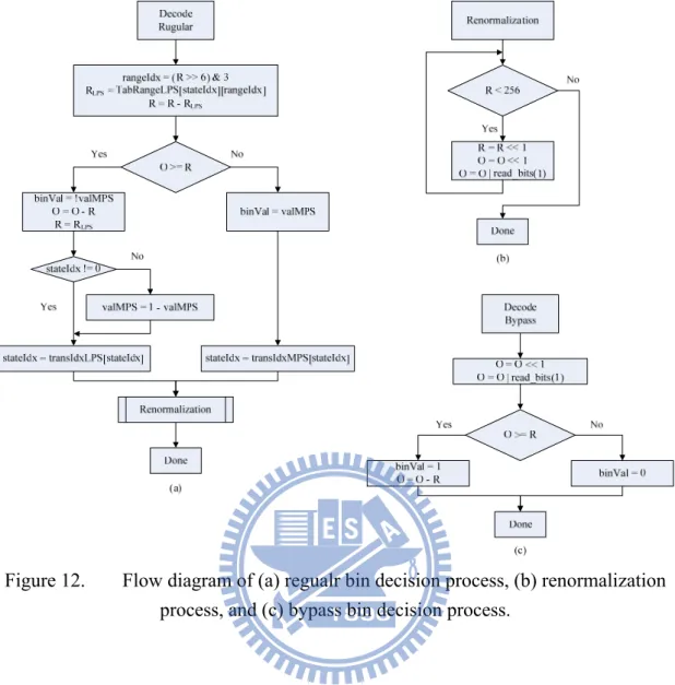
Fig. 12 Flow diagram of (a) regular bin decision process, (b) renormalization process, and (c) bypass bin decision process ... 26
Fig. 13 Pipelining scheme of CABAC decoding ... 27
Fig. 14 Data hazard caused by significance map. (a) 4x4 residual block. (b) Flow diagram of the CABAC decoding scheme for significance map. (c) Example for decoding the significance map. (d) Illustration of cycle stall of CABAC decoding ... 28
(Chapter4) Fig. 15 Framework of proposed entropy decoder ... 31
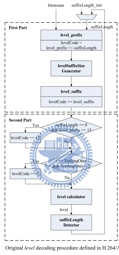
Fig. 16 Original level decoding procedure defined in H.264/AVC standard ... 35
Fig. 17 MSD decoding procedure ... 36
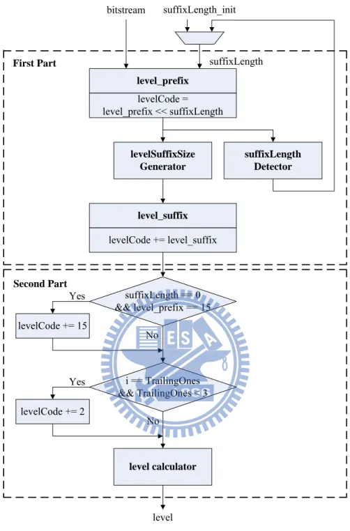
Fig. 18 Modified level decoding procedure with MSD algorithm ... 37
Fig. 19 Proposed delay balanced two-level decoding architecture ... 39
Fig. 20 Proposed CAVLC decoder ... 41
Fig. 21 Residual block reconstruction architecture ... 42
Fig. 23 Proposed CABAC decoder architecture ... 52
Fig. 24 Pipeline scheduling of (a) prediction miss and (b) prediction hit ... 54
Fig. 25 Memory operation in the significance map decoding process ... 61
Fig. 26 Mathematical reordering. (a) O-(R-RLPS). (b) (O-R)+RLPS ... 65
Fig. 27 Mathematical transform for the second bin decision process ... 65
Fig. 28 Architecture of proposed two-symbol arithmetic decoding engine ... 66
(Chapter5) Fig. 29 Framework of proposed entropy decoder for SVC ... 74
List of Tables
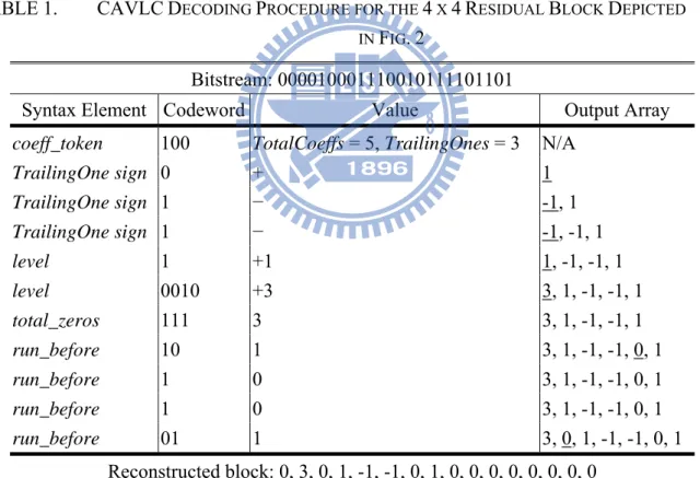
(Chapter2)Table 1 CAVLCDECODING PROCEDURE FOR THE 4 X 4RESIDUAL BLOCK DEPICTED IN FIG.2 ... 7
(Chapter3) Table 2 DECODING PROCUDURE FOR INPUT NUMBER ... 12
Table 3 UNARY BINARIZATION ... 14
Table 4 TRUNCATED UNARY BINARIZATION ... 14
Table 5 FIXED-LENGTH BINARIZATION ... 15
Table 6 UEG3BINARIZATION FOR ABSOLUTE VALUES OF MOTION VEXTOR DIFFERENCES ... 16
Table 7 SYNTAX ELEMENT AND CORRESPONDING CONTEXT INDICES ... 17
Table 8 CONTEXT CATEGORY DEPENDING ON SYNTAX ELEMENTS AND BLOCK TYPES ... 19
(Chapter4) Table 9 THRESHOLD VALUE FOR SUFFIXLENGTH TRANSITION ... 35
Table 10 EXAMPLE OF RESIDUAL BLOCK RECONSTRUCTION PROCESS ... 42
Table 11 COMPARISON OF CAVLCDECODING PERFORMANCE ... 43
Table 12 CAVLCDECODER IMPLEMENTATION RESULT COMPARISONS DIFFERENT DESIGNS ... 44
Table 13 MAXIMUM FRAME RATES FOR SOME EXAMPLE FRAME SIZES ... 44
Table 14 WORKING FREQUENCY FOR DIFFERENT LEVEL CONDITIONS ... 46
Table 15 STATISTICAL RESULT OF BIN DISTRIBUTION WITH ICODING STRUCTURE AND QP28 ... 48
Table 16 STATISTICAL RESULT OF BIN DISTRIBUTION WITH ICODING STRUCTURE AND QP20 ... 49
Table 17 STATISTICAL RESULT OF BIN DISTRIBUTION WITH ICODING STRUCTURE AND QP12 ... 49
Table 18 STATISTICAL RESULT OF BIN DISTRIBUTION WITH IPPPCODING STRUCTURE AND QP28 ... 49
Table 19 STATISTICAL RESULT OF BIN DISTRIBUTION WITH IPPPCODING STRUCTURE AND QP20 ... 50
Table 20 STATISTICAL RESULT OF BIN DISTRIBUTION WITH IPPPCODING STRUCTURE AND QP12 ... 50
Table 21 STATISTICAL RESULT OF BIN DISTRIBUTION WITH IBBBPCODING STRUCTURE AND QP28 ... 51
Table 22 STATISTICAL RESULT OF BIN DISTRIBUTION WITH IBBBPCODING STRUCTURE AND QP20 ... 51
Table 23 STATISTICAL RESULT OF BIN DISTRIBUTION WITH IBBBPCODING STRUCTURE AND
QP12 ... 52
Table 24 IMPROVEMENT OF PREDICTION ACCURACY USING THE PROPOSED METHODS WITH I CODING STRUCTURE ... 55
Table 25 IMPROVEMENT OF PREDICTION ACCURACY USING THE PROPOSED METHODS WITH IPPPCODING STRUCTURE ... 55
Table 26 IMPROVEMENT OF PREDICTION ACCURACY USING THE PROPOSED METHODS WITH IBBBPCODING STRUCTURE ... 56
Table 27 BIN INDEX TRANSITION RELATION IN SIGNIFICANCE MAP ... 57
Table 28 CONTENT OF SRAMAFTER REORGANIZATION OF OUR PROPOSAL ... 61
Table 29 CONTENT OF REGISTER AFTER REORGANIZATION OF OUR PROPOSAL ... 62
Table 30 CABACDECODING PERFORMANCE OF THE PROPOSED ARCHITECTURE WITH ICODING STRUCTURE ... 67
Table 31 CABAC DECODING PERFORMANCE OF THE PROPOSED ARCHITECTURE WITH IPPP CODING STRUCTURE ... 68
Table 32 CABACDECODING PERFORMANCE OF THE PROPOSED ARCHITECTURE WITH IBBBP CODING STRUCTURE ... 69
Table 33 CABACDECODER IMPLEMENTATION RESULT COMPARISONS OF DIFFERENT DESIGNS ... 69
Table 34 WORKING FREQUENCY FOR DIFFERENT LEVEL CONDITIONS ... 70
(Chapter5) Table 35 CONTENT OF SRAM FOR SVCQUALITY ENHANCEMENT LAYER ... 74
Table 36 CONTENT OF REGISTER FOR SVCQUALITY ENHANCEMENT LAYER ... 75
Table 37 CONTENT OF SRAM FOR SVCBASE LAYER ... 75
Table 38 CONTENT OF REGISTER FOR SVCBASE LAYER ... 76
Chapter 1 INTRODUCTION
H.264/AVC is the state-of-the-art video coding standard developed by the Joint Video Team (JVT) of ISO/IEC Moving Picture Experts Group and the ITU-T Video Coding Experts Group (MPEG and VCEG). With many advanced techniques, it provides better compression efficiency for video than the earlier MPEG-4 and H.263 standards do. Recently, H.264/AVC has been widely adopted in current video application system such as Blu-ray Disc, Youtube, television service, and real-time videoconferencing.
H.264/AVC specifies two entropy coding tools: Context-based Adaptive Variable Length Coding (CAVLC), and Context-based Adaptive Binary Arithmetic Coding (CABAC) [1], [2]. Both methods employ context-based adaptive modeling in their entropy coding framework and achieve better compression efficiency compared to previous video coding standards. In CAVLC, an adaptive VLC table switching method depending on already coded symbols is used, and in CABAC, an adaptive probability model estimation technique is utilized for binary arithmetic coding. For the reason that the adaptation of CAVLC can not perfectly match actually conditional symbol statistics and the limitation of 1 bit/symbol imposed on variable length codes, CABAC can achieve averaged bit-rate savings of 9% to 14% at the cost of higher computation complexity in comparison to CAVLC [3].
1.1 Motivation and Contribution
In recent years, as network transmission speed rises and high-definition television gains popularity, the demand for better visual quality grows fast. That means video application system is expected to support high-definition (HD) resolution
encoding and decoding. In addition to the heavy decoding requirement of H.264/AVC, this trend leads to the result that more data has to be processed in the same time for video decoders, and makes it more difficult to work in real-time for CPUs. In that event, it is necessary to accelerate the decoding speed of entropy decoder with hardware since its throughput dominates the overall decoder system performance. However, the inherently strong data dependency significantly restricts the throughput of entropy decoder and is generally considered as the main design challenge in hardware implementation. In order to achieve high decoding performance and low hardware cost real-time entropy decoding systems, a fully hardwired entropy decoder is proposed in this thesis.
1.2 Thesis Organization
The rest of this thesis is organized as follows. We briefly describe the entropy codec (CAVLC and CABAC) and their design challenges in hardware implementation in Chapter 2 and Chapter 3, respectively. In Chapter 4, the proposed entropy decoding architecture is presented and we provide simulation results to demonstrate the performance of our entropy decoder design. In Chapter 5, we extend our proposed entropy decoder towards the Scalable Video Coding (SVC) extension of the H.264/AVC standard. Finally, the conclusion is given in Chapter 6.
Chapter 2 OVERVIEW OF CAVLC
Variable-length coding (VLC) is an entropy coding method that converts each data symbol to a variable length codeword, and achieves data compression by utilizing the various probabilities of occurrence of data symbols. Symbols with high probabilities of occurrence are represented by short codewords while symbols with low probabilities of occurrence are represented by long codewords. There are two constrains on the VLC, one is that the bit string must consist of integral number of bits, another one is that each codeword must be uniquely decodable.
2.1 Context-based Adaptive Variable Length Coding
CAVLC and Exp-Golomb coding are the baseline entropy coding methods of H.264/AVC. In spite of the advantage of Exp-Golomb coding in computational efficiency, the compression efficiency is not good enough for real application alone. To enhance the compression efficiency, a more efficient entropy coding technique CAVLC is designed for encoding quantized transformed coefficients of 4 x 4 and 2 x 2 residual blocks by taking advantage of several characteristics of quantized blocks. After decorrelated by the Discrete Cosine Transform (DCT) and quantization, most of the quantized coefficients are zero while a few nonzero coefficients are clustered around the top left of the block. Afterward, by a reordering, nonzero coefficients are grouped together and the level of nonzero coefficients tends to be larger at the low frequencies (start of the reordered array) and smaller toward the high frequencies (end of the reordered array). Moreover, high-frequency nonzero coefficients are often a series of ±1 (TrailingOnes). To efficiently represent the large number of zeros, a
run-level coding technique can be applied to reduce the redundancy of the data symbols. However, Run and Level are not quite correlated. Consequently, to achieve better compression efficiency, Run and Level are coding separately in CAVLC.
Distinct from conventional VLC that VLC table is unique; CAVLC switches VLC tables for different syntax elements relying on already transmitted symbols. That is why it is named context-based adaptive. Although better compression efficiency is achieved by exploiting inter-symbol redundancies, the rise in computational complexity and data dependency imposed on the CAVLC decoder makes it hard to be speeded up by parallelism and pipelining. In the following, the decoding flow of CAVLC alone with its design challenges is discussed in more detail.
2.1.1 CAVLC Decoding Flow
A residual block is represented by five types of SEs in CAVLC. These syntax elements are defined as follows:
1) coeff_token: This syntax element indicates the total number of nonzero coefficients (TotalCoeffs) including TrialingOnes. Since the coding units of CAVLC are 4 x 4 and 2 x 2 blocks, TotalCoeffs can be any value from 0 to 16 and TrialingOnes can be anything from 0 to 3. There are three variable-length codeword tables and a fixed-length codeword table using for coding coeff_token. The choice of look-up table depends on the total number of nonzero coefficients to the left and on top of the current block, nA and nB respectively.
2) trailing_ones_sing_flag: This 1-bit syntax element indicates the sign of TrialingOnes, and is coded in reverse order.
3) level: The syntax element level represents the value of remaining nonzero coefficients and is also coded in reverse order. Each level is composed of a
prefix part (level_prefix) and a suffix part (suffix_part).
4) total_zeros: The sum of zero coefficients, except for zeros after the last nonzero coefficient, is represented by this syntax element. The choice of VLC table depends on the total number of nonzero coefficients of the current block.
5) run_before: Number of zeros preceding each nonzero coefficient is encoded as this syntax element. The VLC table for coding each run_before is chosen according to the number of zeros left (zerosLeft).
Fig. 1 shows the flow diagram of CAVLC decoding. The decoding process consists of six steps: coeff_token parsing, trailing_ones_sing_flag parsing, level parsing, total_zeros parsing, run_before parsing, and residual block reconstruction. Table 1 shows an example for the decoding procedure of a CAVLC coded residual block as depicted in Fig. 2 and its corresponding decoded information. The input bitstream provided for CAVLC decoder is “00001000_11100101_11101101”, after the decoding procedure, the 4 x 4 residual block, “0, 3, 0, 1, -1, -1, 0, 1, 0, 0, 0, 0, 0, 0, 0, 0”, is reconstructed.
0 3 -1 0 0 1 0 0 0 0 0 0 0 0 -1 1 Reordered block: 0, 3, 0, 1, -1, -1, 0, 1, 0... 4 x 4 residual block
Encoded CAVLC bitstream: 000010001110010111101101
Figure 2. Transmitted bitstream for a 4 x 4 residual block.
TABLE 1. CAVLCDECODING PROCEDURE FOR THE 4 X 4RESIDUAL BLOCK DEPICTED IN FIG.2
Bitstream: 000010001110010111101101
Syntax Element Codeword Value Output Array
coeff_token 100 TotalCoeffs = 5, TrailingOnes = 3 N/A
TrailingOne sign 0 + 1 TrailingOne sign 1 − -1, 1 TrailingOne sign 1 − -1, -1, 1 level 1 +1 1, -1, -1, 1 level 0010 +3 3, 1, -1, -1, 1 total_zeros 111 3 3, 1, -1, -1, 1 run_before 10 1 3, 1, -1, -1, 0, 1 run_before 1 0 3, 1, -1, -1, 0, 1 run_before 1 0 3, 1, -1, -1, 0, 1 run_before 01 1 3, 0, 1, -1, -1, 0, 1 Reconstructed block: 0, 3, 0, 1, -1, -1, 0, 1, 0, 0, 0, 0, 0, 0, 0, 0
2.2 Design Challenges and Related Works
In hardware implementation, the VLC decoding can be realized as a finite state machine in essence. One bit or several bits of bitstream are scanned in each clock
cycle. According to the chosen VLC table, if the bit string matches a codeword, the corresponding value is returned. Otherwise, more bits will be scanned in the next cycle. Since the bitstream boundary between successive codewords is unknown until the codeword length of the former one is detected, the decoding procedure is inherently sequential and thus the throughput of CAVLC decoder is therefore hard to be elevated.
Intuitively, multi-symbol decoding is an effective way to raise throughput, especially for trailing_ones_sing_flag, level, and run_before parsing stages which are critical loops in the CAVLC decoding procedure. However, the main obstacle to parallel decoding is how to break the recursive dependencies between codewords. In trailing_ones_sing_flag parsing stage, since the number of TrailingOnes is already derived in coeff_token parsing stage, [4] and [5] implemented the parsing procedure in a single cycle. In level parsing stage, two level decoders are cascaded to produce two level symbols in one cycle [6]. However, it induces a huge critical path delay. In run_before parsing stage, since the codewords of VLC table used for run_before is much less and shorter than others, the data dependency obstacle is much easier to be overcome, and thus several efficient multi-run_before decoding architectures had proposed to boost the throughput of CAVLC decoder. When run_before is equal to 0, the corresponding codeword is composed of “1” bits. Therefore by counting the bit length of the series of “1” bits of input bitstream, multiple run_before symbols valued 0 can be parsed in one cycle [6]. This method is effective in the high bit-rate coding but inefficient in the low bit-rate coding where the residual blocks are very sparse. Since the sub VLC tables of run_before are separated by zerosLeft, unless zerosLeft is larger than 6, the zerosLeft for choosing the next run_before look-up table is predictable. By utilizing this character, Yu et al. [7] proposed a combined look-up table for decoding successive two run_before symbols at the same time. At the
expense of significant hardware cost raise, Wen et al. [8] adopted a bit-position VLC decoding approach that all run_before symbols are decoded using less than 3 cycles in one block to achieve high throughput. Lee et al. [9] presented a multi-symbol decoder that can decode three run_before symbols in one cycle. Furthermore, a pattern-search method had been reported in [10]. In this method, a block can be reconstructed directly without performing CAVLC decoding procedure if a pattern is matched in a pre-established look-up table.
For the two critical loops, level parsing process and run_before parsing process, which mainly affect the overall decoding performance, a lot of techniques have been proposed to speed up run_before parsing process, whereas there are few effective ways to improve level parsing performance. In this thesis, a highly efficient two-level decoding architecture is proposed to expedite the CAVLC decoding speed.
Chapter 3 OVERVIEW OF CABAC
For a data symbol with probability of occurrence P to be encoded, the theoretical optimum number of bits is log2(1 / P). It is usually a fraction instead of an integer. As
a result, in essence, entropy coding based on integral number of bits long codewords can not achieve optimal data compression. As a practical alternative, arithmetic coding provides a technique that can encode a sequence of data symbols into a single fractional number and thus can more closely approach the theoretical optima.
3.1 Arithmetic Coding
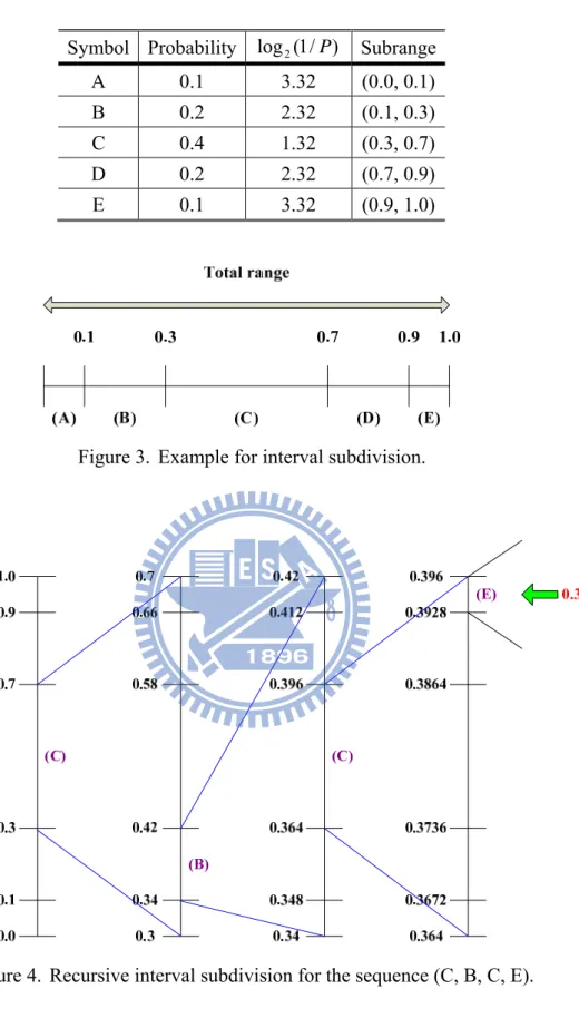
The arithmetic coding algorithm is a recursive subdivision of an interval based on the probability of occurrence of encoded symbols. In the encoding procedure, first, the range (0.0, 1.0) is subdivided into subranges depending on the probability of occurrence of each symbol as Fig. 3 shows. Then, whenever a symbol is encoded, the new rage is set to the corresponding subrange. Finally, the sequence of data symbols can be represented by any fractional number in the final range. An example for encoding the sequence (C, B, C, E) is presented in Fig. 4. After the first symbol is encoded, the new range is (0.3, 0.7), and the next new range is (0.34, 0.42). Progressively, the initial range becomes smaller. At the end of sequence of data symbols, a number 0.394 which lies within the final rage (0.3928, 0.396) is outputted.
Figure 3. Example for interval subdivision.
Figure 4. Recursive interval subdivision for the sequence (C, B, C, E).
In the decoding procedure, each symbol is decoded depending on the subrange where the input number falls. Then, the new range is updated to this subrange. Table 2 shows an example for decoding a fractional number 0.394 encoded by the encoding
Symbol Probability log2(1/P) Subrange
A 0.1 3.32 (0.0, 0.1)
B 0.2 2.32 (0.1, 0.3)
C 0.4 1.32 (0.3, 0.7)
D 0.2 2.32 (0.7, 0.9)
procedure mentioned above. When decoding the first symbol, because 0.394 falls within the subrange (0.3, 0.7), it is decoded as (C). Then, range is set to the subrange which belongs to (C). The next symbol is decoded as (B) since 0.394 lies within the subrange (0.34, 0.42), and so on. The decoding does not halt until the entire sequence of data symbols (C, B, C, E) is decoded.
TABLE 2. DECODING PROCUDURE FOR INPUT NUMBER 0.394
3.2 Context-based Adaptive Binary Arithmetic Coding
In spite of the fact that the algorithm of arithmetic coding is simple in definition, the hardware and software implementations suffer from its high computational complexity. The limited throughput (symbols/second) is generally considered as its main disadvantage. To solve this problem while maintaining the compression efficiency, CABAC introduces an adaptive binary arithmetic coding technique combined with well-designed context models. Furthermore, the interval is subdivided by using addition and look-up take to avoid multiplication operation, and the
Decoding Procedure Range Subrange Decoded Symbol 1) Set the initial range (0.0, 1.0)
2) Find the subrange where the number falls and decode the symbol
(0.3, 0.7) (C)
3) Set the new range (0.3, 0.7) 4) Find the subrange where the number falls
and decode the symbol
(0.34, 0.42) (B)
5) Set the new range (0.34, 0.42) 6) Find the subrange where the number falls
and decode the symbol
(0.364, 0.396) (C)
7) Set the new range (0.364, 0.396) 8) Find the subrange where the number falls
and decode the symbol
probabilities updating is simplified by look-up table.
Fig. 5 shows the block diagram of CABAC encoding process. The encoding process consists of three steps: binarization, context modeling, and binary arithmetic coding [2]. In the first step, a syntax element is transferred from non-binary value into a series of binary bins, called a bin string. For each bin to be encoded, two coding modes are candidates. In the regular mode, a context model representing probability model is first selected according to previous encoded syntax elements. Then, based on the context model, the bin value is encoded by the regular coding engine, and context model updating follows. In the bypass mode, a bypass coding engine without the usage of context model is executed to speed up the encoding process. The three functional blocks are discussed in more detail in the following.
Figure 5. CABAC encoder block diagram.
3.2.1 Binarization
The binarization design in CABAC depends on a few code trees that provide a simple computation to derive codewords. There are four types of binarization process specified in CABAC: the unary (U) binarization process, the truncated unary (TU) binarization process, the fixed-length (FL) binarization process, and the concatenated
unary/ k-th order Exp-Golomb (UEGk) binarization process. However, there is an exception. Instead of computing by means of a structured coding scheme, look-up tables are used for mapping macroblock types and submacroblock types into binary sequences.
Table 3 shows the bin strings of U binarization. For each unsigned integer valued syntax element x, the bin string consists of x “1” bits followed by a terminating “0” bit.
TABLE 3. UNARY BINARIZATION
Value of syntax element (x) Bin string 0 0 1 1 0 2 1 1 0 3 1 1 1 0 4 1 1 1 1 0 5 1 1 1 1 1 0 … … … … … Bin index 0 1 2 3 4 5 …
The bin strings of TU binarization are shown in Table 4. A number cMax is defined for mapping x with [0, cMax]. For x < cMax the bin strings are the same as U codes, whereas x = cMax the bin string is given by a bin string of length cMax with “1” bits only.
TABLE 4. TRUNCATED UNARY BINARIZATION
Value of syntax element (x) Bin string (cMax = 7) 0 0
1 1 0 2 1 1 0 3 1 1 1 0 4 1 1 1 1 0 5 1 1 1 1 1 0 6 1 1 1 1 1 1 0 7 1 1 1 1 1 1 1 Bin index 0 1 2 3 4 5 6
As shown in Table 5, the bin strings of FL binarization are given by fixedLength-bit binary representations, where fixedLength = Ceil( Log2( cMax + 1 ) ). The FL binarization process is mainly applied to the syntax elements which are nearly uniform distribution.
TABLE 5. FIXED-LENGTH BINARIZATION
Value of syntax element (x) Bin string (cMax = 7)
0 0 0 0 1 0 0 1 2 0 1 0 3 0 1 1 4 1 0 0 5 1 0 1 6 1 1 0 7 1 1 1 Bin index 0 1 2
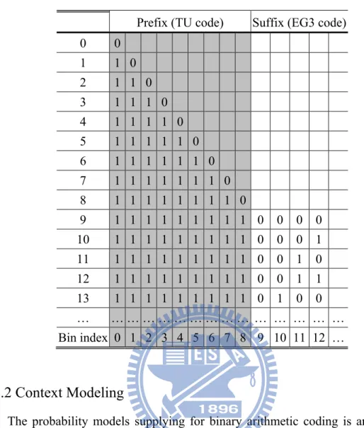
The UEGk binarization process is applied to absolute values of motion vector differences (MVD) and absolute values of transform coefficient levels (ABS_LEVEL). The UEGk bin string consists of a prefix and a suffix code word. The prefix bit string is constructed by TU binarizaton process with cMax = Min( uCoff, Abs( x ) ) , where
ucoff is the cutoff value which also represents the maximum length of the prefix bit string. After the prefix part is obtained, if Abs( x ) is larger than or equal to the cutoff value, the EGk binarization process is invoked to derive the suffix part. The first part of EGk code is formed with a unary code with l(y) = Floor( log2( y / 2k + 1 ) ). The
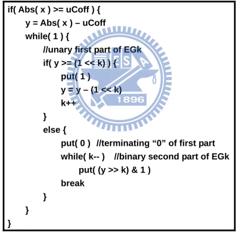
second part is constructed as the binary representation of y + 2k( 1- 2l(y) ) with ( k + l(y) ) bits. The pseudo code of computational procedure is depicted in Fig. 6. Table 6 shows the bin strings for MVD valued from 0 to 13, where the prefix parts are in gray shadow.
if( Abs( x ) >= uCoff ) { y = Abs( x ) – uCoff while( 1 ) {
//unary first part of EGk if( y >= (1 << k) ) { put( 1 ) y = y – (1 << k) k++ } else {
put( 0 ) //terminating “0” of first part while( k-- ) //binary second part of EGk
put( (y >> k) & 1 ) break
} } }
Figure 6. Pseudo code for k-th order Exp-Golomb code construction.
TABLE 6. UEG3BINARIZATION FOR ABSOLUTE VALUES OF MOTION VECTOR
DIFFERENCES
Prefix (TU code) Suffix (EG3 code) 0 0 1 1 0 2 1 1 0 3 1 1 1 0 4 1 1 1 1 0 5 1 1 1 1 1 0 6 1 1 1 1 1 1 0 7 1 1 1 1 1 1 1 0 8 1 1 1 1 1 1 1 1 0 9 1 1 1 1 1 1 1 1 1 0 0 0 0 10 1 1 1 1 1 1 1 1 1 0 0 0 1 11 1 1 1 1 1 1 1 1 1 0 0 1 0 12 1 1 1 1 1 1 1 1 1 0 0 1 1 13 1 1 1 1 1 1 1 1 1 0 1 0 0 … … … … Bin index 0 1 2 3 4 5 6 7 8 9 10 11 12 …
3.2.2 Context Modeling
The probability models supplying for binary arithmetic coding is an important part since it dominates the overall coding efficiency. Consequently, the context model has to be selected by taking into account conditional probability estimation and keep updated during encoding. In CABAC, to reduce the complexity requirement, only the neighbors of current syntax element are involved in context model selection such that only a few choices are left.
TABLE 7. SYNTAX ELEMENTS AND CORRESPONDING CONTEXT INDICES Syntax Element Slice Type
I/SI P/SP B
mb_skip_flag 11–13 24–26
mb_field_decoding_flag 70–72 70–72 70–72 end_of_slice_flag 276 276 276
mb_type 0/3–10 14–20 27–35 transform_size_8x8_flag 399–401 399–401 399–401 coded_block_pattern 73–84 73–84 73–84 mb_qp_delta 60–63 60–63 60–63 prev_intra4x4_pred_mode_flag 68 68 68 rem_intra4x4_pred_mode 69 69 69 prev_intra8x8_pred_mode_flag 68 68 68 rem_intra8x8_pred_mode 69 69 69 intra_chroma_pred_mode 64–67 64–67 64–67 ref_idx 54–59 54–59 mvd (horizontal) 40–46 40–46 mvd (vertical) 47–53 47–53 sub_mb_type 21–23 36–39 coded_block_flag 85–104 85–104 85–104 significant_coeff_flag 105–165, 277–337 105–165, 277–337 105–165, 277–337 last_significant_coeff_flag 166–226, 338–398 166–226, 338–398 166–226, 338–398 coeff_abs_level_minus1 227–275 227–275 227–275 significant_coeff_flag (8x8) 402–416, 436–450 402–416, 436–450 402–416, 436–450 last_significant_coeff_flag (8x8) 417–425, 451–459 417–425, 451–459 417–425, 451–459 coeff_abs_level_minus1 (8x8) 426–435 426–435 426–435
All context models are listed in Table 7. Each context model, which contains a 6-bit probability state and the value of most probable symbol, is identified by a context index (ctxIdx). The calculation of ctxIdx is defined as
ctxIdxInc ctxCat
ctxIdxBase
ctxIdx
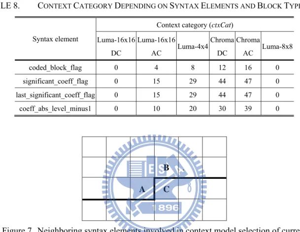
where ctxIdxBase denotes the base context index, which is defined as the lower value of the range contained in Table 7, ctxCat represents context category, which is only valid for syntax elements of residual type and is given in Table 8, and ctxIdxInc denotes the context index increment, which is derived based on bin index (binIdx),
previously encoded bins, or neighboring syntax elements to the left and on top of the current syntax element, as illustrated in Fig. 7.
TABLE 8. CONTEXT CATEGORY DEPENDING ON SYNTAX ELEMENTS AND BLOCK TYPES
Syntax element
Context category (ctxCat) Luma-16x16 DC Luma-16x16 AC Luma-4x4 Chroma DC Chroma AC Luma-8x8 coded_block_flag 0 4 8 12 16 0 significant_coeff_flag 0 15 29 44 47 0 last_significant_coeff_flag 0 15 29 44 47 0 coeff_abs_level_minus1 0 10 20 30 39 0 B . A C
Figure 7. Neighboring syntax elements involved in context model selection of current syntax element.
3.2.3 Adaptive Binary Arithmetic Coding
Binary arithmetic coding is based on the principle of progressive interval subdivision. In terms of symbols to be encoded, only most probable symbol and least probable symbol (MPS and LPS) with probabilities of occurrence PMPS and PLPS are
specified. Based on this setting, the given interval represented by a lower bound (L) and an interval range (R) is subdivided into RMPS and RLPS as follows:
LPS MPS LPS LPS R R R P R R
However, the computational requirement of multiplication operations becomes the bottleneck that limits the overall throughput. To solve this problem, a novel multiplication-free solution with negligible performance degradation is developed in CABAC.
Motivated by introducing some approximations of the range R or of the probability PLPS in substitution for their actual values, the basic idea of the new
multiplication-free binary arithmetic coding scheme for H.264/AVC relies on the assumption that the estimated probabilities of each context model can be represented by a sufficiently limited set of representative values [3]. Total 128 probability states are effectively used for representing the approximate probability estimation of each context model. Each probability state is composed of a 6-bit state index (stateIdx) indicating the LPS probability and a 1-bit value that represent the MPS value (valMPS). The numbering of state index is guided by the principle that with state index equaling to 0 corresponds an LPS probability value of 0.5, the higher the number of state index, the lower LPS probability value is assigned. Whenever the encoding procedure of each symbol is completed, the context model updating process is executed to keep context models “up to date”. The determination of probability updating is illustrated in Fig. 8. In practical implementation, the transition of probability states can be realized by a table-based transition process. This continuous update makes the binary arithmetic coding engine adaptive.
), 1 ( ), , ( 62 old old P P P Max Pnew 095 . 0 0.5 0.01875 63 1
Fig. 9 shows the flow diagram of binary arithmetic encoding process. Two coding modes are specified in CABAC, one is regular coding mode, where probability estimation is utilized, and another one called bypass coding mode is used to encode symbols with approximately uniform probability distribution.
rangeIdx = (R >> 6) & 3 RLPS= TabRangeLPS[stateIdx][rangeIdx] R = R - RLPS binVal != valMPS L = L + R R = RLPS stateIdx != 0 valMPS = 1 - valMPS
stateIdx = transIdxLPS[stateIdx] stateIdx = transIdxMPS[stateIdx]
Done Encode Rugular Yes No Yes No Encode Bypass L = L << 1 L = L + R R = RLPS (a) Done Yes (b) Renormalization Renormalization binVal != valMPS
Figure 9. Flow diagram of binary arithmetic encoding process. (a) Regular coding mode. (b) Bypass coding mode.
Fig. 9(a) illustrates the regular coding mode. In the first step, with a table which contains 64 x 4 pre-computed LPS subranges, the interval range is subdivided depending on the state index and range without multiplication operation. Then, according to the given bin value (binVal), the corresponding process is performed.
Finally, since the interval range has to stay within [28, 29] to keep a fixed precision, a renormalization process is necessary if the updated interval range R is smaller than 0x100. Fig. 10 shows the flow diagram of renormalization process. The output bits are recursively generated during the renormalization. If the interval range is in the bottom half, PutBit(0) is performed; else if the interval range is in the top half, PutBit(1) is performed; otherwise bitsOutstanding (BO) is increased by 1.
With regard to bypass coding mode, the probability distribution of symbol to be encoded is nearly uniform. That means RLPS = RMPS = R/2. Consequently, the usage of
context model is not required and the subdivision operation can be simplified to accelerate the encoding speed. Furthermore, only one-loop renormalization process using double decision thresholds without doubling R and L is performed in the final step. The flow diagram of bypass coding mode is depicted in Fig. 9(b).
Renormalization R < 256 L = L - 256 BO = BO + 1 Done (a) L < 256 L >= 512 L = L - 512 R = R << 1 L = L << 1 PutBit(B) firstBitFlag != 0 firstBitFlag = 0 WriteBits(B, 1) BO > 0 WriteBits(1-B, 1) BO = BO - 1 Done (b) No Yes No Yes No Yes Yes Yes No No PutBit(0) PutBit(1)
3.3 CABAC Decoding Algorithm Overview
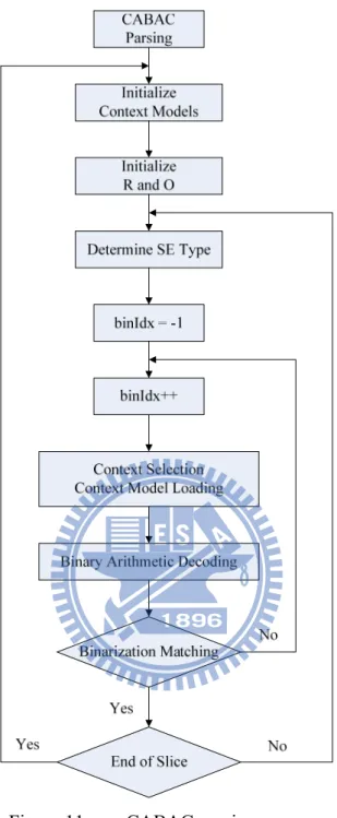
In CABAC, every syntax element (SE) is composed of a series of bins. Given the bitstream, combined with syntax element parsing, the object of CABAC decoder is to transfer the decoded bin string into actual value and return it. Fig. 11 depicts the generic CABAC parsing process. Prior to decoding a new slice, an initialization process is performed that all context models are initialized depending on the slice type and quantization parameter, moreover, the interval range and coding offset are reset to 0x1FE and first 9 bits of the bitstream, respectively. In the parsing flow, each syntax element is parsed sequentially. After the type of syntax element is decided, depending on the bin index, the corresponding bin decoding process is executed. Finally, the constructed bin string is de-binarized. If any codeword is matched, the corresponding value is returned and the decoding procedure for current syntax element is complete.
Figure 11. CABAC parsing process.
In the hardware realization, the bin decoding process consists of four elementary steps: context selection (CS), context model loading (CL), binary arithmetic decoding (BAD), and binarization matching (BM). In the first step, context index which acts as the context model address is calculated. After the address is obtained, a context model (CM) loaded from CM memory is passed to the BAD stage. In BAD stage, a bin is
decoded to be MPS or LPS according to a probability model provided by the CM. Afterward, the constructed bin string is de-binarized in the final stage to decide whether the decoding process of current SE is finished or not, and the context model update (CU) process takes place at the same time.
To read the specific context model from the context model memory, the memory address must be calculated first. Generally, the memory address of each context model is the same as its corresponding context index. However, the organization of context models in H.264/AVC is clearly not the most economical. Therefore, reorganization is allowed to achieve better performance as designer’s wish.
In the binary arithmetic decoding procedure, most symbols are decoded by the regular bin decision process depending on the location of coding offset. Fig. 12(a) shows the flowchart of regular decoding process. In the first step, according to the state index provided by context model and current interval range, LPS subrange is selected from a look-up table and MPS subrange is calculated as RMPS = R – RLPS.
Then, by comparing the coding offset (O) with the MPS subrange (RMPS), if the
coding offset falls within the LPS subrange, the bin is identified as LPS. Otherwise, if the coding offset falls within the MPS subrange, the bin is identified as MPS. In the meanwhile, R and O are assigned to the corresponding subinterval, and the probability state is transferred in the end.
Figure 12. Flow diagram of (a) regualr bin decision process, (b) renormalization process, and (c) bypass bin decision process.
A renormalization operation is required whenever the interval range (R) is out of its legal range (R < 0x100). Fig. 12(b) depicts the flowchart of renormalization. Recursively, the left-shift of R and O does not halt until R is larger than or equal to 0x100. During the renormalization procedure, the input bits coming from bitstream are appended to coding offset.
Besides, the other symbols with approximately uniform probability distribution are decoded by bypass bin decision process. The flowchart of bypass decoding process can be seen in Fig. 12(c).
In hardware implementation, to achieve high throughput, pipelined architecture and parallel architecture are considered helpful methods generally. Since every bin is decoded by the same chain of operations (CS→CL→BAD→BM and CU), the decoding performance can be elevated by exploiting the pipelining scheme presented in [11] . Fig. 13 shows a 4-stage pipelining CABAC decoder design. However, the boost of throughput is limited by the pipeline stalling caused by data hazards. Take significance map (significant_coeff_flag and last_significant_coeff_flag) which occupies the major portion of syntax elements in slice data for example, as shown in Fig. 14, the choice of the bin right after significant_coeff_flag and corresponding context model depends on the current bin value since the bin may be significant_coeff_flag or last_significant_coeff_flag. As a result, two cycles are unavoidable to resolve this data hazards.
Decode coded_block_flag coded_block_flag == 1 Decode significant_coeff_flag Decode last_significant_coeff_flag significant_coeff_flag == 1 last_significant_coeff_flag == 1 Done scanningPosition < numCoeff - 1 scanningPosition = 0 scanningPosition++ Scanning Position Transform coefficient levels significant_coeff_flag last_significant_coeff_flag Yes No Yes No Yes No 0 1 2 3 4 5 6 8 0 -3 0 0 1 1 0 0 0 0 0 0 1 1 1 1 1 (c) (a) CS CL BAD BM CU CS CL BAD BM CU stall stall
binVal CM depends on previous binVal
(d) Yes No 8 -3 0 0 0 1 1 0 0 0 0 0 0 0 0 0 (b)
Figure 14. Data hazard caused by significance map. (a) 4x4 residual block. (b) Flow diagram of the CABAC decoding scheme for significance map. (c) Example for
decodong the significance map. (d) Illustration of cycle stall of CABAC decoding.
To relieve the performance degradation originated in syntax element switching overhead, a prediction-based pipelined architecture was proposed in [12], where the correlation between successive SEs are exploited to achieve higher prediction accuracy in comparison to the prediction that just predicts current symbol to be MPS. Furthermore, multi-symbol decoding architecture design is also an effective way to
speed up decoding procedure. A parallel decoding method was proposed to enhance decoding performance by predicting that the current symbol is MPS [16]. The architecture in [13] employed a branch selection two-symbol parallel decoding technique to resolve data dependency problem, and can process two bins within one cycle for general cases, but suffers from high area cost. Chen et al. [14] proposed a fully hardwired CABAC decoder that is capable of decoding at most two bins in one cycle for certain syntax elements: coeff_abs_level_minus1, significant_coeff_flag, last_significant_coeff_flag, and mvd.
However, in some works such as [15], [16], their architecture only focuses on bin decoding process, while leaving SE parsing to another processor. Although the separation of SE parsing and decoding makes the implementation of CABAC decoding much simpler, it results in that the actual throughput can not reach its theoretical maximum, since whenever SE switching takes place, the context model has to be reloaded.
A fully hardwired CABAC decoder design which combines SE parsing with decoding is proposed in this thesis. The characteristics of SE parsing flow and bin distribution among SEs are analyzed to design the decoding architecture which not only can decode multiple bins in one cycle without stalls for most cases but also can keep low hardware cost by employing hybrid context model memory architecture. Moreover, with the efficient mathematical transform method for two-symbol binary arithmetic decoding (TSBAD) engine, the decoding speed can be further elevated.
Chapter 4 PROPOSED ENTROPY DECODER
Fig. 15 shows the system level architecture of proposed entropy decoder for H.264/AVC. It contains a CAVLC decoder, a CABAC decoder, a SE parser, a neighboring information fetcher, a bitstream fetcher, and a memory controller. According to the entropy coding mode, the SE parser chooses the corresponding decoder to decode SEs. When entropy_coding_mode_flag is equal to 0, SEs of residual blocks are decoded by using the CAVLC decoding scheme, and other SEs are decoded by using the VLC decoding scheme which is included in the CAVLC decoder. When entropy_coding_mode_flag is equal to 1, SEs lying at macroblock layer and below are decoded using the CABAC decoder, and other SEs belonging to slice layer and above are decoded by the VLC decoder.
In the entropy decoding procedure, the bitstream fetcher reads bitstream which is stored in external memory by the memory controller and transmits it to the CAVLC decoder and the CABAC decoder. The neighboring data involving in entropy decoding process, such as total_coeff and mvd used for calculating nC and ctxIdxInc, are stored in the upper macroblock information memory. Furthermore, if entropy coding mode is binary arithmetic coding, in the beginning of decoding each slice, all the CMs are reset to the initial values stored in ROM. Whenever a SE is decoded, if it is related to the remaining SE parsing flow, it will be buffered in the SE register. The detail of our proposed entropy decoder is presented in the following.
Figure 15. Framework of proposed entropy decoder.
4.1 Proposed CAVLC Decoder
It is apparent that the greatest obstacle to further boosting the throughput of CAVLC decoder originates in level parsing procedure which is based on arithmetic operations and accounts for a critical loop in the whole CAVLC decoding procedure. In terms of multi-level decoding, since the inter-codeword dependency and succession of arithmetic operations lead to an unavoidably long critical path, we can not gain throughput from cascading level decoders directly. Moreover, the inter-level dependency of suffixLength which can not be calculated until the value of current level is determined makes it unable to exploit pipeline structure. It seems both multi-symbol decoding and pipelining scheme are not workable for level decoding process.
Our destination is to find a method that can break the inter-level dependency and the inter-codeword dependency. If this goal is reached, we can make a breakthrough
and thus the CAVLC decoding performance can be further improved. Consequently, first of all, we investigate the characteristics of level decoding flow.
4.1.1 Analysis
Fig. 16 shows the flowchart of level decoding procedure defined in the H.264/AVC standard. The decoding procedure can be divided into two parts: the first part is bitstream scanning process and the second part is for computing the value of level. The bit string of each level is formed with level_prefix and level_suffix as
] _ ][ 01 ... 0 [ ] _ ][ _ [ _ suffix level suffix level prefix level bitString level
where level_prefix consists of a series of “0” bits followed by a terminating “1” bit. The value of level_prefix is constrained in the range 0 to 15 in general profiles. In the bitstream scanning process, after the value of level_prefix is determined by detecting the leading zeros in the bitstream, the parameter levelSuffixSize which represented the bit length of level_suffix is calculated as
if(level_prefix = = 15) levelSuffixSize = 12
else if(level_prefix = =14 && suffixLength = = 0) levelSuffixSize = 4
else
levelSuffixSize = suffixLength Based on the levelSuffixSize, bits belonging to level_suffix are scanned, and the initial value of levelCode is calculated as
suffix level th suffixLeng prefix level levelCode( _ ) _
In the second part, levelCode is adjusted in case of special conditions. If level_prefix is equal to 15 and suffixLength is equal to 0, levelCode will be increased by 15, and if the number of TrailingOnes is less than 3, the first levelCode in the level decoding procedure will be increased by 2. Once the final value of levelCode is obtained, the value of level will be determined as: if levelCode is even, level = (levelCode + 2) / 2. Otherwise, level = (-levelCode - 1) / 2. Finally, since the absolute value of level tends to be larger in the level decoding procedure, to obtain high compression efficiency, adaptive probability model is used depending on previous decoded level. As a result, by examining the absolute value of decoded level, if it is larger than the thresholds listed in Table 9, suffixLength must be modified to a more suitable value since small suffixLength is fit for small level; large suffixLength is just the opposite.
The main barriers to exploit parallel decoding are inter-level dependency of suffixLength and the unknown demarcation between successive codewords. Although the codeword length can be derived in the first part of level decoding procedure as follows: xSize levelSuffi prefix level ngth CodewordLe _ 1
, the updated suffixLength which affect the levelSuffixSize of next level can not be obtained until the value of current level is determined. However, a modified suffixLength detector (MSD) algorithm was presented to advance the computation of suffixLength prior to the determination of the value of current level [4]. Fig. 17 depicts the MSD decoding procedure, the input signal of MSD is level_prefix instead of the value of level. From the current decoding information and the level_prefix, the suffixLength provided for next level decoding process can be calculated in the first part. With this efficient algorithm, the level decoding process can be realized as Fig.
18 shows. However, despite the fact that the MSD algorithm shortens the critical path delay of level decoding process, multi-level decoding based on cascaded level decoders still leads to an unavoidably long critical path, and thus remains unsuitable for implementation.
In our approach, to further expedite the throughput of CAVLC decoder, instead of straight cascading level decoders, we take advantage of MSD algorithm to exploit a highly performance two-level decoding architecture. In general case, the levelSuffixSize which indicates the codeword length of level_suffix is equal to suffixLength. Consequently, the start point of next level codeword in the bitstream can be decided as soon as the level_prefix decoding has finished. Moreover, the adjustment of levelCode in the second part is only applied to the first level of the residual block. It means that those two special conditional branches can be skipped in the second level decoding. Base on these two features, we propose a delay balanced two-level decoding (DBTLD) architecture that efficiently shortens the critical path in comparison to traditional design that cascades two level decoders directly.
level_prefix levelSuffixSize Generator level_suffix levelCode = level_prefix << suffixLength levelCode += level_suffix suffixLength == 0 && level_prefix == 15 i == TrailingOnes && TrailingOnes < 3 levelCode += 15 levelCode += 2 Yes No Yes No First Part Second Part bitstream suffixLength level level calculator suffixLength_init suffixLength Detector
Figure 16. Original level decoding procedure defined in H.264/AVC standard.
TABLE 9. THRESHOLD VALUE FOR SUFFIXLENGTH TRANSITION
Current suffixLength Threshold value to modify suffixLength
0 0 1 3
2 6 3 12 4 24 5 48 6 N/A
level_prefix levelSuffixSize Generator level_suffix levelCode = level_prefix << suffixLength levelCode += level_suffix suffixLength == 0 && level_prefix == 15 i == TrailingOnes && TrailingOnes < 3 levelCode += 15 levelCode += 2 Yes No Yes No First Part Second Part bitstream suffixLength suffixLength Detector level level calculator suffixLength_init
Figure 18. Modified level decoding procedure with MSD algorithm.
4.1.2 Proposed Delay Balanced Two-level Decoder Architecture
Fig. 19 shows the block diagram of proposed DBTLD architecture. The second level decoding process is designed for the general case that levelSuffixSize is equal to suffixLength. Since the codeword length of first level can be determined immediately after the level_prefix is decoded, and the examination process of levelCode increment
is unnecessary for the second level decoding process, a balanced structure can be obtained.
The first level decoding process is the same as Fig. 18 shows. For bitstream supplying for the second level decoding process, the input bitstream is shifted according to suffixLength and level_prefix_1. Afterward, instead of generating levelSuffixSize_2, the level_suffix_2 is parsed directly by fetching the output of first suffixLength_1 detector (SD_1) which is referred to the MSD algorithm. Finally, without checking the two special cases for increasing levelCode_2, the level mapping process is performed straight. Compared to the conventional approach of cascading two MSD algorithm based level decoders, the critical path delay of proposed DBTLD engine is improved by 21% (from 3.25ns to 2.56ns).
level_prefix_1 levelSuffixSize Generator level_suffix_1 levelCode_1 = level_prefix_1 << suffixLength levelCode_1 += level_suffix_1 suffixLength == 0 && level_prefix_1 == 15 i == TrailingOnes && TrailingOnes < 3 levelCode_1 += 15 levelCode_1 += 2 Yes No Yes No bitstream suffixLength_1 suffixLength Detector level_1 level calculator level_prefix_2 levelCode_2 = level_prefix_2 << suffixLength_1 level_suffix_2 levelCode_2 += level_suffix_2 Bitstream Shifter level calculator level_2 suffixLength Detector suffixLength_2 suffixLength_init suffixLength First Part Second Part
Figure 19. Proposed delay balanced two-level decoding architecture.
4.1.3 CAVLC Decoding Architecture Design
Based on the DBTLD engine, the CAVLC decoding architecture is designed as shown in Fig. 20. In the trailing_ones_sing_flag decoding unit, all sign flags are scanned in one cycle. After level decoding procedure is done, all nonzero coefficients are stored in a 16-entry deep and 13-bit wide output buffer. Finally, in the run_before decoding unit, whenever a run_before symbol is decoded, the corresponding level is transmitted to its actual position in the output buffer. Since only one output buffer is
used instead of storing level and run_before information separately, to regularize the data transmission of output buffer, the prediction-based run_before look-up table combination method [7] is employed that two run_before symbols are decoded in one cycle except when only one run_before symbol left. Fig. 21 shows the architecture of residual block reconstruction. After TrailingOnes and levels are pushed in the output buffer in order, in each cycle, one or two level symbols are moved to their final locations respectively depending on the coeffsLeft and zerosLeft information. The movement starts from the last coefficient and ends until no more run_befores are decoded. The parameters coeffsLeft denotes the remaining number of nonzero coefficients needs to be moved, and zerosLeft represents the remaining number of zeros to be decoded. Table 10 shows an example for the reconstruction process. In the beginning, all nonzero coefficients are arranged in order, output buffer index 0 to (TotalCoeffs – 1). After total_zeros is decoded, coefficients are moved to the indices which are calculated as (coeffsLeft + zerosLeft – 1) in reverse order, and the value of the original position of the moved coefficient is replaced by 0. In this example, first, the last coefficient 1 is moved to index 8 (6 + 3 - 1), and the coefficient -1 is moved to index 6 (5 + 2 - 1). In the next cycle, only the one run_before symbol is valid since no more zeros left to be decoded, and the coefficients -2 is moved to index 4 (4 + 1 - 1).
To further accelerate the decoding procedure, skipping mechanism is employed to remove redundant decoding processes:
1) Zero block skip: When TotalCoeffs is equal to 0, the remaining decoding processes are skipped since nonzero coefficients do not exist in the block. 2) Level skip: When TotalCoeffs is equal to TrailingOnes, the level decoding
procedure is skipped since there has no nonzero coefficients left to be decoded.
coefficients (maxNumCoeff), the total_zeros decoding procedure and run_before decoding procedure is bypassed because there are no zero coefficients to be decoded.
4) Run skip: When total_zeros is equal to 0 or TotalCoeffs is equal to 1, run_before decoding procedure is not necessary.
Moreover, in the CAVLC decoding procedure, because coeff_token, trailing_ones_sing_flag, level, total_zeros, and run_before decoding units are not performed simultaneously, only one of them is designated to work in each cycle, to save power consumption, idled units are turned off by functional gating.
Figure 21. Residual block reconstruction architecture.
TABLE 10. EXAMPLE OF RESIDUAL BLOCK RECONSTRUCTION PROCESS
Decoded Symbol coeffsLeft zerosLeft Output Buffer
total_zeros = 3 x x 4 3 2 -2 -1 1 0 0 0 0 0 0 0 0 0 0 run_before_1 = 1 run_before_2 = 1 6 3 4 3 2 -2 0 0 -1 0 1 0 0 0 0 0 0 0 run_before_1 = 1 run_before_2 = x 4 1 4 3 2 0 -2 0 -1 0 1 0 0 0 0 0 0 0
4.1.4 Experimental Results
Table 11 shows the decoding performance of the proposed CAVLC decoder for different video sequences. To compare with previous works fair, we use the same testing environment that all the sequences with resolution of QCIF (176 x 144) are intra coded. The RTL simulation result shows in the low bit-rate coding like high QP or simple image, since the residual block is very sparse, Lee’s design [9] which only focus on boosting run_before decoding procedure can achieve higher decoding speed. However, in the high bit-rate coding, the demand for high decoding speed is actually necessary, our proposed design that takes both level and run_before decoding procedures into consideration prevails over other existing designs.
hardware cost and decoding speed with other existing work are shown in Table 12. The proposed CAVLC decoder is synthesized with UMC 90nm. We enhance the throughput by exploiting multi-symbol decoding scheme for both level and run_before symbols while allowing the maximum working frequency to be about 390 MHz with 13.88k gate count. Lin’s design [4] has minimum hardware cost, however, its decoding speed of the two main critical loops, level decoding procedure and run_before decoding procedure that dominate the overall decoding performance, is only one symbol per cycle, which is merely half in comparison to our design. By applying the prediction-based run_before look-up table combination method [7], two run_bofore symbols can be decoded in each cycle. Furthermore, with the DBTLD engine, not only two level symbols can be decoded at the same cycle, but also 21% critical path delay is saved in comparison to the traditional two-level decoder. Table 13 shows the maximum frame rates (frames per second) for different Level limits defined in the H.264/AVC standard. According to the definition and the throughput of our design, we list the minimum working frequency requirement of Level in Table 14. The result shows that our proposed CAVLC decoder can achieve real-time decoding for all Level conditions.
TABLE 11. COMPARISON OF CAVLCDECODING PERFORMANCE
Video Sequence QP Bitrate(Mbps) Average cycle/MB Proposed Yu [7] Lee [9] Tsai [6] Akiyo 28 0.59 44 50 N/A 39 20 1.13 75 93 N/A N/A 12 2 117 154 N/A 143 Foreman 28 0.83 58 68 N/A N/A 20 1.76 116 151 N/A N/A 12 3.12 182 259 N/A N/A Mobile 28 2.21 145 194 135 150
20 3.66 203 300 211 N/A 12 5.32 233 367 264 241 News 28 0.83 58 70 49 N/A 20 1.53 95 125 87 N/A 12 2.58 141 195 138 N/A Stefan 28 1.5 102 133 97 106 20 2.58 150 214 154 N/A 12 3.94 188 282 204 201 Average 127.13 177 148.8 146.67 Reduction (%) 28.18 14.56 13.32
TABLE 12. CAVLCDECODER IMPLEMENTATION RESULT COMPARISONS OF DIFFERENT
DESIGNS
Specifications Proposed Lin [4] Yu [7] Lee [9] Alle [5] Tsai [6] Technology 90nm 0.18um 0.18um 0.18um 0.13um 0.13um 0.18um Max. Frequency 385 MHz 193 MHz 213 MHz 125 MHz 125MHz 250MHz 160 MHz Area: Logic Part
(gate count) 13,544 14,373 6,771 13,192 15,602 17,202 13,189 Area: Memory Part
(bits) W/O W/O W/O W/O 5,120 W/O
Average cycle/MB 127.13 N/A 177 148.8 N/A 146.67
Level 1 1b 1.1 1.2 1.3 2 2.1 2.2 3 3.1 3.2 4 4.1 4.2 5 5.1 Max MBs/frame 99 99 396 396 396 396 792 1620 1620 3600 5120 8192 8192 8704 22080 36864 Format Resolution (W x H) MBs Total SQCIF 128x96 48 30.9 30.9 62.5 125.0 172.0 172.0 172.0 172.0 172.0 172.0 172.0 172.0 172.0 172.0 172.0 172.0 QCIF 176x144 99 15.0 15.0 30.3 60.6 120.0 120.0 172.0 172.0 172.0 172.0 172.0 172.0 172.0 172.0 172.0 172.0 QVGA 320x240 300 - - 10.0 20.0 39.6 39.6 66.0 67.5 135.0 172.0 172.0 172.0 172.0 172.0 172.0 172.0 525 SIF 352x240 330 - - 9.1 18.2 36.0 36.0 60.0 61.4 122.7 172.0 172.0 172.0 172.0 172.0 172.0 172.0 CIF 352x288 396 - - 7.6 15.2 30.0 30.0 50.0 51.1 102.3 172.0 172.0 172.0 172.0 172.0 172.0 172.0 525 HHR 352x480 660 - - - - - - 30.0 30.7 61.4 163.6 172.0 172.0 172.0 172.0 172.0 172.0 625 HHR 352x576 792 - - - - - - 25.0 25.6 51.1 136.4 172.0 172.0 172.0 172.0 172.0 172.0 VGA 640x480 1200 - - - 16.9 33.8 90.0 172.0 172.0 172.0 172.0 172.0 172.0 525 4SIF 704x480 1320 - - - 15.3 30.7 81.8 163.6 172.0 172.0 172.0 172.0 172.0 525 SD 720x480 1350 - - - 15.0 30.0 80.0 160.0 172.0 172.0 172.0 172.0 172.0 4CIF 704x576 1584 - - - 12.8 25.6 68.2 136.4 155.2 155.2 172.0 172.0 172.0 625 SD 720x576 1620 - - - 12.5 25.0 66.7 133.3 151.7 151.7 172.0 172.0 172.0 SVGA 800x600 1900 - - - 56.8 113.7 129.3 129.3 172.0 172.0 172.0 XGA 1024x768 3072 - - - 35.2 70.3 80.0 80.0 172.0 172.0 172.0 720p HD 1280x720 3600 - - - 30.0 60.0 68.3 68.3 145.1 163.8 172.0 4VGA 1280x960 4800 - - - 45.0 51.2 51.2 108.8 122.9 172.0 SXGA 1280x1024 5120 - - - 42.2 48.0 48.0 102.0 115.2 172.0 525 16SIF 1408x960 5280 - - - 46.5 46.5 98.9 111.7 172.0 16CIF 1408x1152 6336 - - - 38.8 38.8 82.4 93.1 155.2 4SVGA 1600x1200 7500 - - - 32.8 32.8 69.6 78.6 131.1 1080 HD 1920x1088 8160 - - - 30.1 30.1 64.0 72.3 120.5 2Kx1K 2048x1024 8192 - - - 30.0 30.0 63.8 72.0 120.0 2Kx1080 2048x1088 8704 - - - 60.0 67.8 112.9 4XGA 2048x1536 12288 - - - 48.0 80.0 16VGA 2560x1920 19200 - - - 30.7 51.2 3616x1536 3616x1536 21696 - - - 27.2 45.3 3672x1536 3680x1536 22080 - - - 26.7 44.5 4Kx2K 4096x2048 32768 - - - - 30.0 4096x2304 4096x2304 36864 - - - - 26.7
![Fig. 5 shows the block diagram of CABAC encoding process. The encoding process consists of three steps: binarization, context modeling, and binary arithmetic coding [2]](https://thumb-ap.123doks.com/thumbv2/9libinfo/7634540.136024/28.892.139.761.527.820/diagram-encoding-process-encoding-consists-binarization-modeling-arithmetic.webp)