First-order analysis of a three-lens afocal zoom system

First-order analysis of a three-lens afocal zoom

system

Mau-Shiun Yeh Shin-Gwo Shiue

Mao-Hong Lu,MEMBER SPIE

National Chiao Tung University Institute of Electro-Optical Engineering 1001 Ta Hsueh Road

Hsin Chu 30050, Taiwan E-mail: mhlu@jenny.nctu.edu.tw

Abstract. A general analysis for the first-order design of a three-lens afocal zoom system with one lens fixed is presented. The reasonable solution areas in the focal length diagrams with positive or negative mag-nification are derived and shown graphically. The relation between the two separations of the three lenses in zooming is found to be a hyper-bola. According to the different locations of hyperbola centers, four cases are analyzed. From the four hyperbolic graphs, we get five different types of zoom systems. For each zoom type, we find the maximum range of magnification and the position where the maximum or minimum system length occurs during zooming. The zoom loci for the first or sec-ond lens fixed are also discussed. © 1997 Society of Photo-Optical Instrumenta-tion Engineers. [S0091-3286(97)02204-6]

Subject terms: zoom lenses; zoom design.

Paper 33076 received July 30, 1996; revised manuscript received Nov. 13, 1996; accepted for publication Nov. 14, 1996.

1 Introduction

A zoom system is generally considered to consist of three parts: the focusing, zooming and fixed parts. The focusing part is placed in front of the zooming part to adjust the object distance. The zooming part is literally used for zooming and the fixed rear part serves to control the focal length or magnification and reduce the aberrations of the whole system. Several of the published papers1concerning zoom have concentrated on the first-order zoom design. We also proposed a two-optical-component method for design-ing zoom system and a first-order analysis for the two-conjugate zoom system.2,3

An afocal zoom system is one in which the entrance and exit marginal rays are parallel to the optical axis. For a typical afocal zoom system, at least three lenses are needed with one lens fixed and the other lenses moving. The first lens is referred to as the focusing part and the others are the zooming part. Although different types of afocal zoom sys-tems have been designed and widely used in many optical systems, such as telescopes, viewing finders, optical scan-ning systems, etc., few of the related publications4–10 dis-cuss their solution distribution. Chuang et al.11 discussed the solution areas of a three-lens afocal zoom system ac-cording to the combinations of focal length values of the three lenses. They described the relation between magnifi-cation and either of the two separations of lenses in zoom-ing.

In this paper, we use the graphoanalytical method12 to solve the first-order layout of the three-lens afocal zoom system. The possible solution areas in the focal length dia-gram are shown graphically for positive and negative mag-nifications. We find the relation between the two separa-tions of lenses in zooming, which can be described with a hyperbola. We obtain four hyperbolas corresponding to the different positions of hyperbola centers in the interlens separation coordinate system. From the four hyperbolic

graphs, we can get five types of zoom systems and find the maximum range of magnification for each zoom type. The zoom position where the system has the maximum or mini-mum length is described. We discuss the zoom loci with the first or central lens fixed.

2 Theory

2.1 Basic Formulas

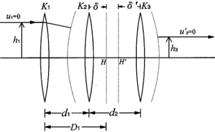
The afocal zoom system, consisting of three lenses with one lens fixed and the others moving, has been analyzed with the two-optical-component method,2in which the first lens is considered as one component and lenses 2 and 3 are combined as the second component. For an infinite-conjugate system, as shown in Fig. 1, the second focal point of lens 1 coincides with the first focal point of the combined unit. The related equations are then given by

D15F11F235d11d, ~1! d5F_F23 3 d2, ~2! K235K21K32K2K3d2, ~3! M52 F1 F235 h1 h3 , ~4!

where K and F are the equivalent power and focal length of a lens, respectively. The combined component has the focal length F23 and power K23; d1 and d2 are the separations between lenses 1 and 2 and between lenses 2 and 3, respec-tively; M is the magnification of system;d is the distance

from the first lens to the first principal plane H of the com-bined unit of lenses 2 and 3; and h is the height of marginal ray at lens.

Solving the preceding equations, we have

d₁5F₁1F₂1F1F2 F3M , ~5! d25F21F31 F₂F₃M F1 . ~6!

In zooming, we change M and then obtain d₁ and d₂. The results are suitable for the case in which any one of the three lenses is fixed during zooming. Because the afocal system with the front lens fixed is the reverse case with the rear lens fixed, the analyses for these two cases are the same. Thus we discuss only the system with the first or second lens fixed in zooming.

2.2 Solution Areas in the Focal Length Diagram Rewrite Eqs.~5! and ~6! as

d15a11 b₁ M, ~7! d25a21b2M , ~8! where a15F11F2, b15 F1F2 F3 , a25F21F3, and b25 F2F3 F₁ .

The separations d₁ and d₂ must be positive in zooming. This provides some constraints on the solutions for a₁, a₂, b₁, b₂, and M in the focal length diagram. From Eq.

~5!, we have

F11F21

S

D

F1F2>0. ~9!

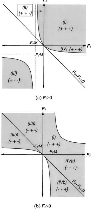
In the F1 versus F2 coordinate graph, the curve

F11F21F1F2/(F3M )50 is a hyperbola with its center at (2F3M ,2F3M ). The solution distribution in the graph is divided into several areas by the hyperbolic curves. Each solution area has different solution ranges for M and d₁.

Similarly, we have the following inequality equation from Eq.~6!.

F21F31

S

M F1

D

F2F3>0. ~10!

In the F2 versus F3 coordinate graph, the curve

F21F31(M/F1)F2F350 is also a hyperbola with its cen-ter at (2F₁/ M ,2F₁/ M ). The solution distribution in the graph is also divided into several areas by the hyperbolic curves. Each solution area has different solution ranges for M and d2.

From the preceding analysis, we can illustrate the pos-sible solution areas in the focal length diagrams according to the different combinations of F1, F2, F3 and the sign of

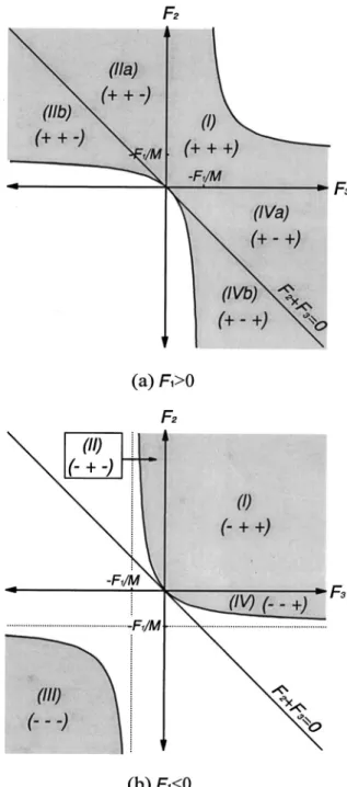
M . Figs. 2 and 3 show the solution areas with positive M under the conditions of positive d₁ and d₂, respectively. The signs of three lens powers in each area are shown in parentheses as (F1,F2,F3). The signs of a1(5F11F2) in Fig. 2 and a2(5F21F3) in Fig. 3 are positive in the upper-right section and negative in the lower-left section of coor-dinate graph. Similarly, Figs. 4 and 5 show the solution areas with negative M for positive d1 and d2, respectively. 2.3 Relation Between M and the Interlens

Separation d1or d2

The relation between M and one of the two interlens sepa-rations can be drawn with Eq. ~5! or Eq. ~6!. Chuang et al.11described the results in their paper. The relations are hyperbolic between M and d₁ and linear between M and d₂.

2.4 Relation Between the Two Interlens Separations d₁ and d₂

From Eqs.~5! and ~6!, we have

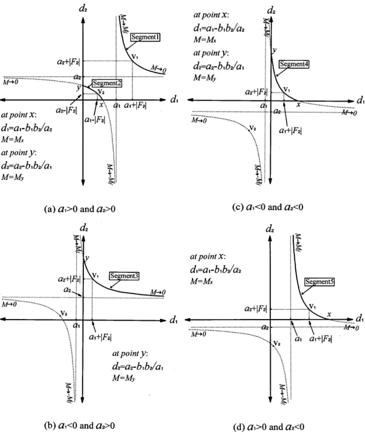
@d12~F11F2!#@d22~F21F3!#5F2 2 , ~11! or ~d12a1!~d22a2!5F2 2 . ~12!

The preceding equation describes a hyperbola with its cen-ter at the coordinates (a1,a2) in the d1 to d2 coordinate graph. Because the center of hyperbola can be located in any quadrant, we obtain four cases of hyperbolas shown in

Fig. 1 Gaussian diagram of three-lens afocal zoom system:d(d8) is the distance from the first (second) lens to the first (second) princi-pal planeH(H8) of the combined unit.

Figs. 6~a! to 6~d! depending on the signs of a₁ and a₂. From Eqs.~7! and ~8!, we can solve the magnification for each point on the hyperbola in Fig. 6, given by

M5 b1 d12a1 , ~13! or M5d22a2 b₂ . ~14!

In Eq.~13!, if d1 approaches the infinity, the magnification

M approaches zero. If d2 in Eq.~14! approaches the infin-ity, the magnification M approaches the infinity and the sign of M is determined by the sign of d2/b2. If

b2(5F2F3/F1).0, the magnifications for points on the upper-right hyperbolic curve are positive and on the lower-left hyperbolic curve are negative. On the other hand, if b2,0, the magnifications for points on the upper-right and lower-left hyperbolic curves are negative and positive, re-spectively.

Fig. 2 Solution areas (shadowed) for different combinations of lens

types with positiveM, and (a)F3.0 and (b)F3,0 under the

con-dition of positived₁.

Fig. 3 Solution areas for different combinations of lens types with

positiveM, and (a)F_1.0 and (b)F_1,0 under the condition of posi-tived₂.

In Fig. 6, the intersections of hyperbola and the two axes are x and y corresponding to d250 and d150, respectively. From Eq.~14! with d250, the magnification at point x is

Mx52 a2

b2

. ~15!

Substituting Eq.~15! into Eq. ~13! at point x, we have

d15a12

b1b2

a₂ . ~16!

Similarly, the magnification Myand the value of d2at point

y are obtained with d₁50 in Eq. ~13!. We have

My52 b₁ a1 , ~17! d25a22 b1b2 a1 . ~18!

In fact, the separations d1 and d2 must be positive in zooming simultaneously. Thus only the segments of

hyper-Fig. 4 Solution areas for different combinations of lens types with

negative M, and (a)F_3.0 and (b) F_3,0 under the condition of positived1.

Fig. 5 Solution areas for different combinations of lens types with

negative M, and (a)F_1.0 and (b) F_1,0 under the condition of positived₂.

bola in the first quadrant of the d₁ versus d₂ coordinate graph are acceptable and are shown with solid lines in Fig. 6. Five possible segments are found and marked by ‘‘Seg-ment’’ followed by a number. Each segment represents the

characteristics of a zoom system, including the constraints on a₁ and a₂ ~i.e., on F₁, F₂, F₃! and the solution ranges of d1, d2, and M in zooming. Therefore, we can have five types of zoom systems.

Fig. 6 Diagramsd1versusd2for the centers of hyperbolas located in the four quadrants, respectively;

V₁andV₂are the vertexes of hyperbola. The magnificationM_fis the plus infinity if (F₂F₃/F₁).0 and the minus infinity if (F₂F₃/F₁)_,0. The intersection coordinates of hyperbola and two axes arexand y, respectively.

From the property of hyperbola, the value of d₁1d₂has the minimum at the vertex V₁ with d₁5a₁1uF₂u and d₂5a₂1uF₂u for segments 1, 3, 4, and 5 and has the maxi-mum at the vertex V2 with d15a12uF2u and

d25a22uF2u for segment 2. Thus the system length, which is the distance from lens 1 to lens 3, has an extreme value

~maximum or minimum! at some position of zooming, i.e.,

not necessarily at the one end of zooming, if the vertex of hyperbolic curve falls in the first quadrant. In this case, the magnification M is calculated as follows.

Substituting d15a11uF2u or d25a21uF2u into Eq.~13! or~14! for segments 1, 3, 4, and 5, we have

M5F1

F₃ if F2.0, ~19!

M52F1 F3

if F2,0. ~20!

Similarly, substituting d15a12uF2u or d25a22uF2u into Eq.~13! or ~14! for segment 2, we have

M52F1 F3 if F2.0, ~21! M5F1 F3 if F₂,0. ~22!

On the other hand, if the vertex of hyperbolic curve is outside the first quadrant, the maximum and minimum sys-tem lengths occur at the two ends of zooming.

For the lower-left hyperbolic curve in Fig. 6~a! or the upper-right hyperbolic curve in Fig. 6~c!, the vertex can be located in any quadrant. If the vertex falls in the third rant, the whole hyperbolic curve is outside the first quad-rant. Hence segment 2 or segment 4 disappears and no solution exits. If the vertex falls in the second or fourth quadrant, then the solution range of zooming is determined by the part that is in the first quadrant. So it is possible that no solution exits if the hyperbolic curve is outside the first quadrant.

2.5 Common Solution Areas for Positive d1and d2

From Sec. 2.2 and Sec. 2.4, we find that the solution ranges of M and d1 ~or d2) for each solution area in Figs. 2 and 4 ~or Figs. 3 and 5! are always a part of hyperbola in Fig. 6,

where d₁ ~or d₂) is positive. So we can combine the solu-tion areas in Figs. 2 and 3 to obtain 12 common solusolu-tion areas with positive magnification M . Each of them repre-sents an overlapped solution area where d₁and d₂are both positive. Similarly, we can obtain 11 common solution ar-eas with negative magnification M from Figs. 4 and 5. The results are shown in Tables 1 and 2.

Tables 1 and 2 also show the constraints on the signs of a1 and a2, the used segment of hyperbola in the d1 versus

d2 coordinate graph, and the possible vertex locations of related hyperbolic curve in the four quadrants for each common solution area. The various quadrants are denoted

by I, II, III, and IV, respectively. The maximum ranges of M and the related ranges of d1 and d2 are also described.

For the third and sixth combinations in Table 1, segment 2 in Fig. 6~a! is used and the vertex of related hyperbolic curve is located in the fourth and second quadrants, respec-tively. In those two cases, we have b2,0 ~or

F₂F₃/F₁,0), so the magnifications of points on the lower-left hyperbolic curve in Fig. 6~a! are positive. The solution exists only if segment 2 exists; in this case, My

< Mx is a necessary condition. Similar cases occur in the second, fifth, tenth and twelfth combinations in Table 1. For the tenth and eleventh combinations in Table 2, no solution exists because the vertex of related hyperbolic curve always falls in the third quadrant.

2.6 Five Types of Zoom Systems

As has been mentioned, each of the five segments in Fig. 6 represents the characteristics of a zoom system. Five differ-ent types of zoom systems are thus discussed as follows. 2.6.1 Type I

For segment 1 in Fig. 6~a!, the range of system magnifica-tion can be from plus or minus infinity to zero depending on the sign of b2. Because the vertex of related hyperbolic curve is located in the first quadrant, the system length always passes through a minimum value during zooming. In this case, we choose the second common solution area in Table 2 as an example. According to the constraints on F1, F2, and F3 in the solution areas marked with~IVa! in Fig. 4~a! and ~IVa! in Fig. 5~a!, we give F151,

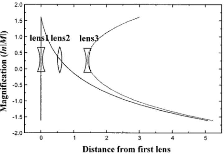
F2520.5, and F351.1. The maximum range of magnifi-cation can be from minus infinity to zero. Here we choose the range of M from 210 to 20.1 with a zoom ratio of 100:1. When the system length has the minimum value, we have d151.000, d251.100, and M520.909. The lens loci in zooming with the first lens fixed are shown in Fig. 7, with the natural logarithm of the magnification as ordinate. If the system with the second lens fixed is used, the zoom loci are as shown in Fig. 8.

2.6.2 Type II

For segment 2 in Fig. 6~a!, the range of system magnifica-tion is from M_x to M_y. Here we choose the second com-mon solution area in Table 1 as an example. Under the constraints on F1, F2, and F3 in the solution areas marked with ~IV! in Fig. 2~a! and ~IV! in Fig. 3~a!, we give F151, F2520.3, and F351.2. So we have Mx52.500 at d150.600 and d250, and My50.357 at d150 and

d250.771. The system has the maximum length with

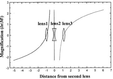
d150.400, d250.600, and M50.833. The zoom loci with the first lens fixed are shown in Fig. 9. If the system with the central lens fixed is used, the lens loci in zooming are as shown in Fig. 10.

2.6.3 Type III

For segment 3 in Fig. 6~b!, the range of system magnifica-tion is from My to 0. In this type, the vertex of hyperbolic curve can be located in the first or second quadrant. Here we use the ninth common solution area in Table 1 as an example. Referring to the solution areas marked with~IIb! Yeh, Shiue, and Lu: First-order analysis . . .

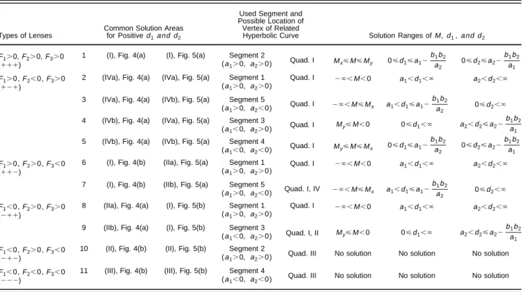
Table 1 Solutions for three-lens afocal zoom system with positive magnification.

Types of Lenses

Common Solution Areas for Positived1andd2

Used Segment and Possible Location of Vertex of Related

Hyperbolic Curve Solution Ranges ofM, d1, andd2 F1.0,F2.0,F3.0

(111)

1 (I), Fig. 2(a) (I), Fig. 3(a) Segment 1

(a_1.0,a_2.0) Quad. I 0,M,` a1,d1,` a2,d2,`

F1.0,F2,0,F3.0 (121)

2 (IV), Fig. 2(a) (IV), Fig. 3(a) Segment 2

(a_1.0,a_2.0) Quad. I–IV IfM_My<Mx, then y<M<Mx 0<d1<a12 b1b2 a2 0<d2<a22 b1b2 a1 F1.0,F2.0,F3,0 (112)

3 (I), Fig. 2(b) (II), Fig. 3(a) Segment 2

(a1.0, a2.0) Quad. IV IfMy<Mx, then My<M<Mx 0<d1<a12 b1b2 a2 0<d2<a22 b1b2 a1 F1.0,F2,0,F3,0 (122)

4 (IVa), Fig. 2(b) (III), Fig. 3(a) Segment 5 (a1.0, a2,0)

Quad. IV Mx<M,` a1,d1<a12 b1b2

a2 0<d2,` 5 (IVb), Fig. 2(b) (III), Fig. 3(a) Segment 4

(a1,0, a2,0) Quad. IV IfMx<My, then Mx<M<My 0<d1<a12 b1b2 a2 0<d2<a22 b1b2 a1 F1,0,F2.0,F3.0 (211)

6 (II), Fig. 2(a) (I), Fig. 3(b) Segment 2

(a1.0, a2.0) Quad. II IfMy<Mx, then My<M<Mx 0<d1<a12 b1b2 a2 0<d2<a22 b1b2 a1 F1,0,F2.0,F3,0 (212)

7 (IIa), Fig. 2(b) (IIa), Fig. 3(b) Segment 1

(a1.0, a2.0) Quad. I 0,M,` a1,d1,` a2,d2,` 8 (IIa), Fig. 2(b) (IIb), Fig. 3(b) Segment 5

(a1.0, a2,0)

Quad. I, IV Mx<M,` a1,d1<a12 b1b2

a2 0<d2,` 9 (IIb), Fig. 2(b) (IIa), Fig. 3(b) Segment 3

(a1,0, a2.0)

Quad. I, II 0,M<My 0<d1,` a2,d2<a22 b1b2

a1 10 (IIb), Fig. 2(b) (IIb), Fig. 3(b) Segment 4

(a1,0, a2,0) Quad. I–IV IfMx<My, then Mx<M<My 0<d1<a12 b1b2 a2 0<d2<a22 b1b2 a1 F1,0,F2,0,F3.0 (221)

11 (III), Fig. 2(a) (IVa), Fig. 3(b) Segment 3

(a1,0, a2.0) Quad. II 0,M<My 0<d1,` a2,d2<a22 b1b2

a1 12 (III), Fig. 2(a) (IVb), Fig. 3(b) Segment 4

(a1,0, a2,0) Quad. II IfMx<My, then Mx<M<My 0<d1<a12 b1b2 a2 0<d2<a22 b1b2 a1

Table 2 Solutions for three-lens afocal zoom system with negative magnification.

Types of Lenses

Common Solution Areas for Positived1and d2

Used Segment and Possible Location of Vertex of Related

Hyperbolic Curve Solution Ranges ofM, d1,and d2 F1.0,F2.0,F3.0

(111)

1 (I), Fig. 4(a) (I), Fig. 5(a) Segment 2

(a1.0, a2.0) Quad. I Mx<M<My 0<d1<a12 b1b2 a2 0<d2<a22 b1b2 a1 F1.0,F2,0,F3.0 (121)

2 (IVa), Fig. 4(a) (IVa), Fig. 5(a) Segment 1 (a1.0, a2.0)

Quad. I <sub>2`,</sub>M,0 a1,d1,` a2,d2,` 3 (IVa), Fig. 4(a) (IVb), Fig. 5(a) Segment 5

(a1.0, a2,0) Quad. I 2`,M<Mx a1,d1<a12 b1b2

a2 0<d2,` 4 (IVb), Fig. 4(a) (IVa), Fig. 5(a) Segment 3

(a1,0, a2.0)

Quad. I My<M,0 0<d1,` a2,d2<a22 b1b2

a1 5 (IVb), Fig. 4(a) (IVb), Fig. 5(a) Segment 4

(a1,0, a2,0) Quad. I My<M<Mx 0<d1<a12 b1b2 a2 0<d2<a22 b1b2 a1 F1.0,F2.0,F3,0 (112)

6 (I), Fig. 4(b) (IIa), Fig. 5(a) Segment 1 (a1.0, a2.0)

Quad. I 2`,M,0 a1,d1,` a2,d2,` 7 (I), Fig. 4(b) (IIb), Fig. 5(a) Segment 5

(a1.0, a2,0) Quad. I, IV <sub>2`,</sub>M<Mx a1,d1<a12 b1b2 a2 0<d2,` F1,0,F2.0,F3.0 (211)

8 (IIa), Fig. 4(a) (I), Fig. 5(b) Segment 1 (a1.0, a2.0)

Quad. I <sub>2`,</sub>M,0 a1,d1,` a2,d2,` 9 (IIb), Fig. 4(a) (I), Fig. 5(b) Segment 3

(a1,0, a2.0) Quad. I, II My<M,0 0<d1,` a2,d2<a22 b1b2

a1 F1,0,F2.0,F3,0

(212)

10 (II), Fig. 4(b) (II), Fig. 5(b) Segment 2

(a1.0, a2.0) Quad. III No solution No solution No solution F1,0,F2,0,F3,0

(222)

11 (III), Fig. 4(b) (III), Fig. 5(b) Segment 4

in Fig. 2~b! and ~IIa! in Fig. 3~b!, we give F1521,

F250.79, and F3520.75. We then have My55.016 at d150 and d253.012. In example, we choose M from 5.016 to 0.200. The system has the minimum length with d150.580, d250.830, and M51.333. The zoom loci with the first lens fixed are shown in Fig. 11.

2.6.4 Type IV

For segment 4 in Fig. 6~c!, the range of system magnifica-tion is from My to Mx. Here we use the tenth common solution area in Table 1 as an example. According to the solution areas marked with ~IIb! in Fig. 2~b! and ~IIb! in Fig. 3~b!, we give F1521, F250.75, and F3521. So we have Mx50.333 at d152.000 and d250, and My53.000 at d150 and d252.000. The system has the minimum length with d150.500, d250.500, and M51.0. The zoom loci with the first lens fixed are shown in Fig. 12.

2.6.5 Type V

For segment 5 in Fig. 6~d!, the range of system magnifica-tion is from plus or minus infinity to Mxdepending on the sign of b2. In this type, the vertex of hyperbolic curve can be located in the first or fourth quadrant. We choose the third common solution area in Table 2 as an example. Re-ferring to the solution areas marked with~IVa! in Fig. 4~a! and ~IVb! in Fig. 5~a!, we give F151, F2520.66, and

F350.52. We then have Mx520.408 at d153.451 and

d250. In example, we choose the range of M from 210.200 to 20.408 with a zoom ratio of 25:1. When the

system has the minimum length during zooming, we get d151.000, d250.520, and M521.923. The zoom loci with the first lens fixed are shown in Fig. 13.

3 Discussion

In this analysis, the graphoanalytical method12 was used because of its convenience to show the connection between the solution space and the variable space used by the lens designer. For designing a zoom system, the size of system and the slope of lens loci are taken into account. In types I

Fig. 7 Loci of three-lens afocal zoom system with F151,

F2520.5, F351.1, and zoom ratio5100. This system has

d₁₅1.000, d₂₅1.100, and M₅₂0.909 at the position where the system length is minimum.

Fig. 8 Loci of three-lens afocal zoom system with the second lens

fixed. The system parameters are the same as in Fig. 7.

Fig. 9 Loci of three-lens afocal zoom system with F₁₅1, F₂₅₂0.3, F₃₅1.2, and zoom ratio₅7. This system has d150.400,d250.600, andM50.833 at the position where the

sys-tem length is maximum.

Fig. 10 Loci of three-lens afocal zoom system with the second lens

fixed. The system parameters are the same as in Fig. 9. Yeh, Shiue, and Lu: First-order analysis . . .

and II, two different results for the zoom loci with the first or second lens fixed are shown. Comparing Fig. 7 with Fig. 8 or comparing Fig. 9 with Fig. 10, we find that the system with the first lens fixed is more compact than that with the second lens fixed. This result is also true for types III to V since the relation between the two interlens separations is similar to that in type I. From the five types of systems, we find that only type II has the result that the maximum sys-tem length occurs inside the process of zooming. In some examples, we have the interlens separation equal to zero at one end of zooming. Usually, it is not useful to work in the neighborhood of the end in practical design. Note that we use the natural logarithm of the magnification as ordinate in Figs. 7 to 13. If the second lens is fixed during zooming, the third lens moves linearly according to Eq.~6!. In this paper, we have not discussed the special condition in which a150 (F11F250) or a250 (F21F350) or both. The solution is easily obtained by the same way as described in

Sec. 2. In this case, the center of hyperbola in Eq.~12! is located on the axis in the d₁ versus d₂ coordinate graph.

4 Conclusion

As we know, a proper first-order layout will often give a satisfactory lens design. For the first-order design of three-lens afocal zoom system, we have analyzed the possible solutions areas in the focal length diagram, the relation be-tween M , d1, and d2, and the properties of lens loci during zooming. The common solution areas for positive d1 and

d2 and their solution ranges of system parameters with positive or negative magnification have been presented. The analysis of five system types, corresponding to five segments in the d1 versus d2 coordinate graph, is helpful for designers to select the positive and negative types of three lenses, preview the shape of lens loci, and determine the ranges of M , d1, and d2.

Acknowledgments

This project was supported by the National Science Council of the Republic of China under the grant No. NSC-85-2215-E-009-004.

References

1. Allen Mann, Ed., Selected Papers on Zoom Lenses, SPIE Milestone Series, Vol. MS 85, SPIE Press, Bellingham, WA~1993!.

2. M. S. Yeh, S. G. Shiue, and M. H. Lu, ‘‘Two-optical-component method for designing zoom system,’’ Opt. Eng. 34~6!, 1826–1834

~1995!.

3. M. S. Yeh, S. G. Shiue, and M. H. Lu, ‘‘First-order analysis of a two-conjugate zoom system,’’ Opt. Eng. 35~11!, 3348–3360 ~1996!. 4. A. Mann, ‘‘Infrared zoom lens system for target detection,’’ Opt. Eng.

21~4!, 786–793 ~1982!.

5. M. Roberts, ‘‘Compact infrared continuous zoom telescope,’’ Opt.

Eng. 23~2!, 117–121 ~1984!.

6. I. A. Neil, ‘‘General purpose zoom lenses for the thermal infrared,’’

Proc. SPIE 518, 55–56~1984!.

7. M. Shechterman, ‘‘High performance wide magnification range IR zoom telescope with automatic compensation for temperature ef-fects,’’ Proc. SPIE 1442, 276–285~1990!.

8. R. Chen, X. Zhou, and X. Zhang, ‘‘Design of compact IR zoom telescope,’’ Proc. SPIE 1540, 717–723~1991!.

9. R. E. Fischer and T. U. Kampe, ‘‘Actively controlled 5:1 afocal zoom

Fig. 11 Loci of three-lens afocal zoom system with F1521,

F250.79, F3520.75, and zoom ratio525. This system has

d₁₅0.580,d₂₅0.830, andM₅1.333 at the position where the sys-tem length is minimum.

Fig. 12 Loci of three-lens afocal zoom system with F1521,

F250.75,F3521, and zoom ratio59. This system hasd150.500,

d250.500, andM51.0 at the position where the system length is

minimum.

Fig. 13 Loci of three-lens afocal zoom system with F151,

F2520.66, F350.52, and zoom ratio525. This system has

d₁₅1.000, d₂₅0.520, and M₅₂1.923 at the position where the system length is minimum.

attachment for common module FLIR,’’ Proc. SPIE 1690, 137–152

~1992!.

10. R. B. Johnson and Chen Feng, ‘‘Mechanically compensated zoom lenses with a single moving element,’’ Appl. Opt. 31~13!, 2274–2278

~1992!.

11. F. M. Chuang, M. W. Chang, and S. G. Shiue, ‘‘Solution areas of three-component afocal zoom system,’’ Optik 101~1!, 10–16 ~1995!. 12. M. L. Oskotsky, ‘‘Grapho-analytical method for the first-order design of two-component zoom systems,’’ Opt. Eng. 31~5!, 1093–1097

~1992!.

Mau-Shiun Yeh received his BS from the

National Taiwan Normal University and his MS from the National Central University. In 1997, he received his PhD in electro-optical engineering from National Chiao-Tung University. He is currently an associ-ate researcher in optical lens design and metrology at the Chung Shan Institute of Science and Technology.

Shin-Gwo Shiue received his BS and MS

degrees from the Chung-Cheng Institute of Technology, Taiwan, in 1973 and 1976, and a PhD degree from the University of Reading, United Kingdom, in 1984. He be-came an assistant researcher at the Chung Shan Institute of Science and Technology in 1976. Before receiving his PhD degree, his research interest was mainly solid state laser physics and after-ward he concentrated in optical instrument design. He was a president of Taiwan Electro-Optical System com-pany in 1990 and joined the Precision Instrument Developing Center of the National Science Council as a senior researcher in 1994. His current research is optical instrument developing, optical metrology, and lens design.

Mao-Hong Lu graduated from the

Depart-ment of Physics at Fudan University in 1962. He was a research staff member at the Shanghai Institute of Physics and Technology, Chinese Academy of Sci-ences, from 1962 to 1970 and at Shanghai Institute of Laser Technology from 1970 to 1980. He studied at the University of Ari-zona as a visiting scholar from 1980 to 1982. He is currently a professor and di-rector at the Institute of Electro-Optical Engineering, National Chiao-Tung University.