不對稱跳躍與不完全資訊對於信用風險模型之影響

國 立 交 通 大 學

財 務 金 融 所

碩 士 論 文

不對稱跳躍與不完全資訊對於信用風險模型之影響 

What Are the Impacts of Asymmetric Jumps and Noisy

Information on the Credit Risk Model?

研 究 生：任 萱

指導教授：郭家豪 博士

不對稱跳躍與不完全資訊對於信用風險模型之影響 

What Are the Impacts of Asymmetric Jumps and Noisy

Information on the Credit Risk Model?

研 究 生：任 萱 Student：Hsuan Rern

指導教授：郭家豪 博士 Advisor：Dr. Jia-Hau Guo

國立交通大學

財務金融研究所碩士班

碩士論文

A Thesis

Submitted to Graduate Institute of Finance National Chiao Tung University in partial Fulfillment of the Requirements

for the Degree of Master of Science

in Finance June 2010

不對稱跳躍與不完全資訊對於信用風險模型之影響 

研究生：任 萱 指導教授：郭家豪 博士

國立交通大學財務金融研究所碩士班

2010年6月

摘要

此篇論文的主旨為在資訊不完全的市場下，建立一個以雙邊指數型跳

躍過程為基礎的信用風險模型、推導此模型下之破產機率，並探討不

對稱跳躍與不完全資訊對於破產機率、破產強度、以及信用利差之衝

擊。研究結果顯示，相較於未考慮跳躍過程之模型，在此含有跳躍過

程之一般化模型的假設下，所求得之信用利差的時間結構更為豐富且

多元。亦即，此篇論文建構之模型將對於真實市場有較佳之解釋能力。

關鍵字：信用風險；不完全資訊；雙邊指數型跳躍過程；破產機率；

信用利差；破產強度；時間結構。

What Are the Impacts of Asymmetric Jumps and Noisy Information on

the Credit Risk Model?

Student : Hsuan Rern Advisor : Dr. Jia-Hau Guo

Institute of Finance

National Chiao Tung University

ABSTRACT

The pure diffusion approach for credit risk model with noisy information is generalized in this paper by including jumps in the firm-value processes. The explicit solution of the default probability for this credit risk model is derived, and the impacts of asymmetric jumps and noisy information on the credit risk are illustrated with numerical results on the default probability, the default intensity, and the credit spread. With the term structure of credit spreads being enriched, our approach is potential to interpret empirical data in real world.

Keywords: credit risk; noisy information; double exponential jump; default probability;

Content

Chinese Abstract ...i

English Abstract ...ii

Content...iii

List of Tables ...iv

List of Figures ...v

1. Introduction... 1

2. The Basic Model ...2

3. An Analysis of the Credit Risk Model ...7

3.1. Default Probability ...7 3.2. Default Intensity...10 3.3. Credit Spreads ...12 4. Conclusions ...13 Reference ...15 Appendix ...30  

List of Tables

Table 1a. Comparison between Monte Carlo simulation and explicit solution of

default probability (λ=0.01)...17 Table 1b. Comparison between Monte Carlo simulation and explicit solution of

List of Figures

Figure 1. Probability of first passage time, for different arrival rate of jump and

different probability of upward jump...18 Figure 2a. Conditional density of V , for different standard deviation of noise _t

( =0.01, p=0.5) ...19 Figure 2b. Conditional density of V , for different standard deviation of noise (_t  =3, p=0.5) ... 20 Figure 2c. Conditional density of V , for different standard deviation of noise (_t  =3, p=0.7) ... 21 Figure 3. Default probability for time horizon 1 year, varying standard deviation of noise ...22 Figure 4a. Default intensity, for different probabilities of upward jump, with noiseless and noisy information . ...23 Figure 4b. Default intensity, for different arrival rates of jump, with noisy

information ...24 Figure 4c. Default intensity, for different arrival rates of jump and varying standard deviation of noise (Vˆ_t 86) ...25

Figure 4d. Default intensity, for different arrival rates of jump and varying standard deviation of noise (Vˆ_t 80) ...26 Figure 5. Credit Spread, for different arrival rates of jump, with noiseless and noisy information...27 Figure 6. The default probability, with noiseless and noisy information ...29

1. Introduction

Default risk analysis plays a critical role in managing the credit risk of bank loan portfolios. In recent research, there are two types of default risk that have been widely used for modeling credit risk. One is the jump risk. For instance, Zhou (1997) and Scherer(2005) incorporates jump risk into the default process and suggests that a firm, the assets of which are perfectly observable, can default instantaneously because of a sudden drop in its value, and the short credit spread of this firm is also bounded away from zero. Another is the default risk due to noisy information. Duffie and Lando(2001) indicates the impacts of the noisy information on the default intensity and the yield spread, and shows that a firm, the asset value of which follows a pure diffusion process but can not be observed directly, can default instantaneously either. However, how do the two types of default risk affect the credit risk model in the same time remains open, and this paper intends to focus on the simultaneous impacts of the asymmetric jumps and noisy information on credit risk.

According to Kou(2002), the double exponential jump-diffusion can capture the empirical phenomenon, which is the asymmetric leptokurtic features that the return distribution is skewed to the left and has a higher peak and two heavier tails than those of pure Brownian motion. With the mean sizes and the probabilities of upward and downward being set respectively, the double exponential jump-diffusion is considered asymmetric and therefore appropriate to capture more realistic jump.

In this paper, a double jump-diffusion process is chosen as the basic model for the asset value of a firm and the noisy information assumption proposed by Duffie and Lando (2001) is incorporated for incomplete information market. The impacts of asymmetric jumps and noisy information on the credit risk are illustrated with numerical results on the default probability, the default intensity, and the credit spread. The result of our analysis shows that the term structure of credit spreads is enriched by simultaneously incorporating the asymmetric jump and the noisy information into the credit risk model. This generalization could be more potential to interpret empirical data in future.

The remainder of this paper is organized as follows. The incorporation of the double exponential jump-process for the asset value of the firm into the credit risk model is given, and then the default probability of the modeled firm is analytically derived in section 2. In section 3, the analysis of the credit risk model is provided for several cases with different arrival rates of jump and information quality to show how asymmetric jumps and noisy information simultaneously influence the default probability, default intensity, and credit spreads. Section 4 concludes this paper.

2. The Basic Model

This section presents our basic model of a firm with noisy information about the credit quality of its debt. We derive the conditional distribution of firm’s assets, given noisy information,

along with the associated default probability.

According to Duffie and Lando(2003), after issuance, bond investors are not kept informed of the status of the firm. Although they do understand that optimizing equity owners will force liquidation when assets fall to v, they can not observe the actual asset level of the company (V ). Instead, they observe the noisy report of assets (_t Vˆ_t). We suppose that the value

of a company follow a stochastic process V 

 

V_{t t0}, and X U , V Vˆ log Z _{t t} 0 t t         where t

U follows a normal distribution with mean  and variance _{a and is independent of} 2 t

X .

The return process _

      0 t t _V V log

X is supposed to follow a double exponential jump-diffusion.

Under the physical probability measure  , the process is given by:



           Nt 1 i i t 2 t t W Y 2 X    , X =0 (1) ₀

where W is a standard Brownian motion, _t N is a Poisson process with rate _t  , and

 

Y _i is a sequence of independent identically distributed (i.i.d.) nonnegative random variables that has an asymmetric double exponential distribution with the density

  y 0 y 2 0 y y 1 Y(y) p e I q e I f 1 2    _  _  _  _{. The constants 1, 0;p,q0, pq1} 2 1   . All

randomness, N , _t W , and _t Y are assumed to be independent; the drift _t  and the volatility  are assumed to be constant, and the Brownian motion and jumps are assumed to be one

dimensional. Furthermore, the moment generating function of X_t is

 

 t, : E

 

e Xt exp



G

 

 t



 

_                    p q 1 2 1 2 1 : G 2 2 1 1 2 2 2              . (2)

The information filtration

 

H_t available to the secondary market is defined by H_t 





Z

 

t₁ ,_,Z

 

t_n ,_{ s} :0st





, for the largest n such that t_n  , where t

 

v inf



t v



 : :V_t

 , the first time that the asset falls below v.

The main objective in this section is to compute the default probability. Firstly, define



x₀,xt,



 as a probability of event that



:  



0

  X 0 s t min _s t s 0 , conditional on V0  and v0 x X_t  ; that is



x0,x, t







₀min_stXs 0X0 x0,Xt x0



, V0 v0 







* *



t * * t * s t s 0 dx X dx X , X max         0 (3) where * _s s X X  . The distribution of * t

X and the joint distribution of the process * t

X and

its running maxima 

 s t s

0 X

max , used in (3) can be computed by the differentiations of the cumulative distribution function of *

t

X and the joint cumulative distribution of * t X and   s t s 0 X

max respectively. The cumulative distribution function of * t

X and the joint cumulative distribution of * t X and   s t s 0 X

max are given by





_                     _{x lim}



_{t W}



_{Y x} X n 1 j j t mn 0 n n mn t     



_{1 2}





_{1 2}



0 L ,p,q, , M ,p,q, , t t x _{     }     _                     (4) and











  



         X  ,X x  X x  maxX  ,X x max _{s t} t s 0 t t s t s 0 0   0 







 

  



       _{     }  X x maxX maxX_s ,X_t x t s 0 s t s 0 t 0 0 -1    (5) where _          2 2  

 ,  , YY which have the distribution as

  y 0 y 2 0 y y 1 Y(y ) p e I q e I f 1 2                  where 1 2 0,2 11;p'q,q' p , and n

 , L



,p,q,₁,₂



, and M



,p,q,₁,₂



are provided in appendix A.



maxX_s b



t s 0      and



maxX_s b,X_t x



t s 0      

 can be computed explicitly from their Laplace transforms. The

Laplace transforms of the two cumulative distributions can be written as





_                    _   



                           1, b 2, , 1 , 2 , 1 1 1 , 2 b , 1 , 2 , 2 1 , 1 1 0 0 s t s t _{maxX bdt} 1 _{e e} e , (6) and









 



 





 









 





,p,q, , ,b,x



F e 0 ; c , , h H b , , , q , p , B e x , b , , , q , p , E x , b , , , q , p , D e x , b , C b , , , q , p , B b , , , q , p , A dt x X , b X max e 2 1 h 0 2 1 h 2 1 2 1 h 2 1 2 1 0 0 s t s t t 2 1 1                                       _{ }           



₍₇₎

where _1,,_2, are the only two positive roots of the equation G

 

 defined in (2), and A, B, C, D, E, F are given in appendix A. Since the cumulative distributions of the first passage times are given in terms of Laplace transforms, numerical inversion of Laplace transforms becomes necessary. To do this, the Gaver-Stehfest algorithm, which does the inversion on the real line, is used in this paper. For any bounded and continuous function f

 



defined on



0,



, f

 

t lim ~f_n

 

t

n

 ,

 

 

 

 

  

 

 



 





     _                                               n 1 k ^ ) 2 n , k min( ) 1 k ( 2 1 j 2 n 2 n k n n t 2 ln k f k j 2 j k 1 j j j 2 n j 2 j 1 t 2 ln lim t f ~ ! ! ! ! ! ! (8)

and f~ is the Laplace transform of f , i.e.

 





 

 

0

t_{f t dt}

e f

~_  _.

Next, the density b



Z_t,x₀ t,



of X , given _t V₀  and “killed” at v₀  inf



t:X_t x



where x is set to be _      0 v v

log , conditional on the observation Z_t  X_tU_t, can be

calculated. By definition,



xz,x0 t,



dx



t,Xt dxZt dz



, x x V0 v0 b       and 



 

 





Z dz



x z dx X t, x x , x t U t           (9) where _U denotes the density of U and _t





_                   





   z Y U W t 2 z Z n 1 j j t t 2 0 n n t        





 



1 2



2 1 2 1 2 1 2 0 , , q , p , M 2 e , , q , p , L 2 e t 2 z 2 2 2 1 2 1                                                        (10) where _2 _2_ta2_.





2 1, , q , p ,

L   , M



,p,q,₁,₂



, and the proof of (12) are given in appendix B.















  v 0 0 0 dx t, x , z x b dx t, x , z x b t, x , z x g . (11)

Finally, the H –conditional default probability is given by _t





_











     v s t,x x g xz,x0 t, dx t s p   (12) where







 

h



0 0 s h t t h s h tminX xX x ΡmaxX X V v Ρ x x , t s               0 0 0 ,  (13) where    0 0 s s X , X X .

3. An Analysis of the Credit Risk Model

In order to analyze how the combination of the noisy information and the asymmetric jump brings the impacts on the credit risk model, we provide several cases for the default probability, the default intensity, and the credit spread with different arrival rates of jump (λ) and standard deviations of noise (a). In these case, the initial asset level given one year ago

0

V =86.3 and the default boundary v78 . We also suppose in all case that U has _t expectation

2 a2

 

 , so that E

 

eUt 1 implies an unbiased asset report. For the jump-diffusion process, r=0.05, σ0.05, 0.02 1 η 1 , and 0.03 12 η 1

. Our basic case is

% 10

a . All parameters refer to Duffie and Lando(2001) and Kou and Wang(2003).

3.1 Default Probability

standard deviation of noise and different jumps to analyze the cooperative impacts of the asymmetric jump and noisy information on the default probability.

Table 1a and 1b compare the explicit solution computed by (14) with the Monte Carlo simulation in the two cases of λ0.01 and λ3. The simulation is based on 1,000,000 simulation runs.

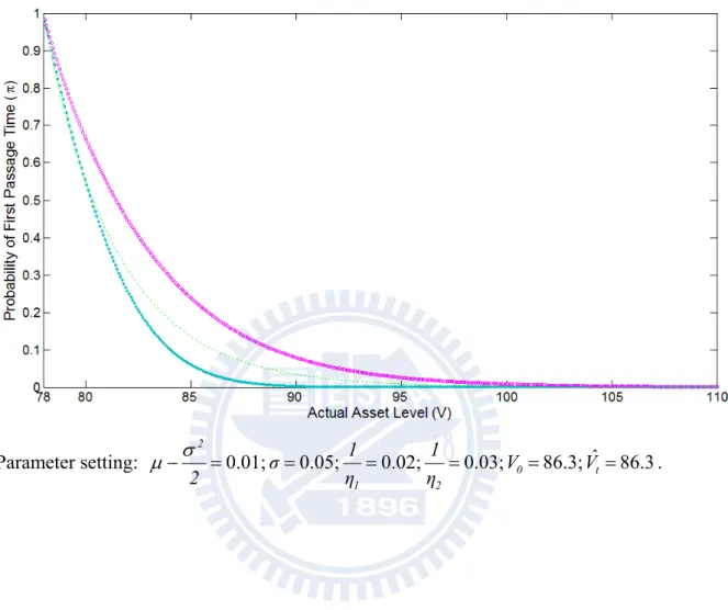
Figure 1 shows the probability of first passage of a double exponential jump diffusion from an initial condition V_t  v0 given v to a level below ₀ v before time s. In order to emphasize the result affected by the jump frequency and the probability of upward jump, the case of λ=3 with symmetric jump is compared with the case of λ=0.01 with symmetric jump, which is near to without jump and the case of λ=3 with asymmetric jump (p=0.7). The previous year’s asset level is set to be 86.3 arbitrarily. As can be seen from Figure 1, given a jump-condition, the probability of first passage time decreases in the actual asset level v at time t, which is in line with our intuition. Furthermore, given the same actual asset level v at time t, the probability of first passage time increases in jump frequency but decreases in the probability of upward jump, which is also in line with our intuition.

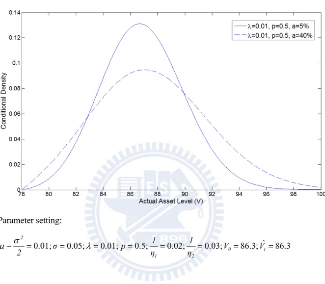
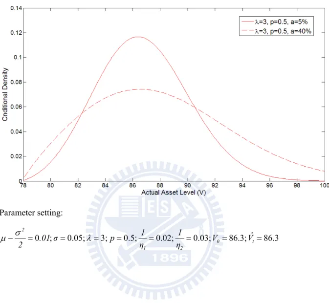
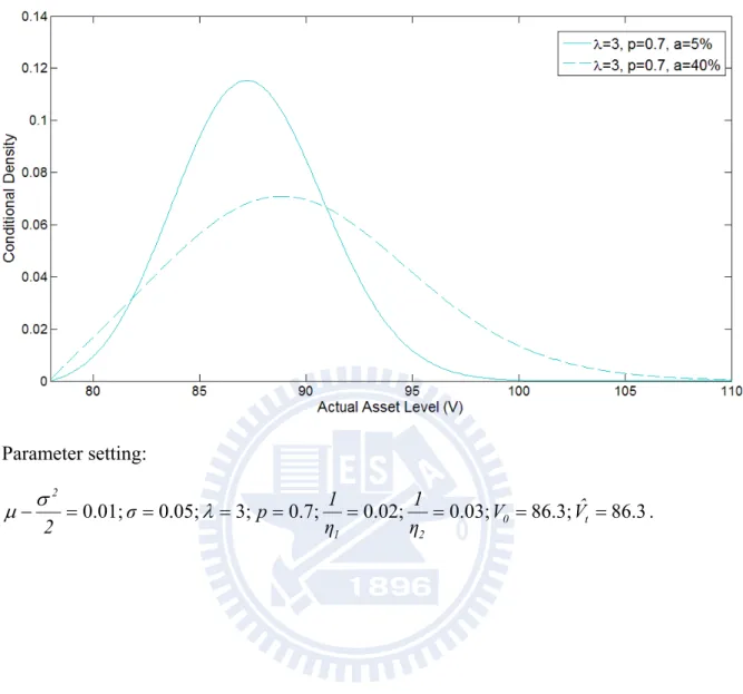
Figure 2a, Figure 2b, and Figure 2c show the conditional density of the current asset level V , given _t H , that would be realized in the event that the bond has not yet default and _t the current asset level reported Vˆ_t has a outcome equal to the previous year’s report. There are three cases of different jump-conditions considered here. One is λ=0.01, p=0.5 (shown

in Figure 2a); another is λ=3, p=0.5 (shown in Figure 2b); still another is λ=3, p=0.7 (shown in Figure 2c). And the standard deviation of noise is set as 5% and 40% for all cases. The previous year’s asset level is set to be 86.3 arbitrarily. It can be shown that in all cases, the density becomes flattened as the standard deviation of noise (a) increases, and the peak density is shifted to the right with jump, p=0.7, which is asymmetric and favoring upward. It is worthy to note that the amount of this shift due to asymmetric jump is magnified by the dubious level of information. It seems that the asymmetric jump cooperates with the information noise and creates a composite effect on the conditional density.

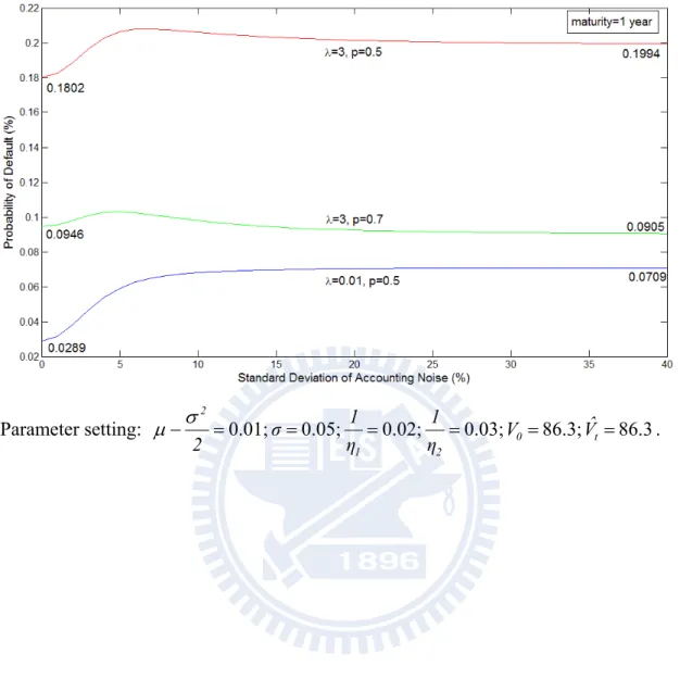
Figure 3 illustrates outcomes of the conditional default probability for cases of different jumps and various levels a of noise. One is for λ0.01and p=0.5; another λ3 and p=0.5; and the other λ3 and p=0.7, given the same previous year asset level of 86.3. For the case of λ0.01, representing a jump of once per hundred year, which is considered rare to happen, the curve we obtained is quite close to that obtained by Duffie and Lando (2001). It means that our generalized model can be reduced to Duffie and Lando’s model. The default probability will increase first and then converge to a certain level as the standard deviation of noise increases. This is because the noise affection will eventually saturate if the standard deviation of noise is large enough. For λ3and p=0.5, the whole curve of the default probability is raised by the jump, and the point probability of the curve increases first as in the case of λ=0.01, reaches the peak value, and then decreases to converge to a saturation level

as the information become more and more dubious. For the case of λ3and p=0.7, the whole curve of the default probability is lowered with respect to the case of λ3and p=0.5, because the asymmetric jump favors upward by assumption; there is also a decrease-to-saturation phenomenon in this case of asymmetric jump. The decrease-to-saturation phenomenon is the result of cooperation of the jump and noisy information. As shown in the equation (12), the default probability is equal to the inner product of the probability of first passage time 



st,xx



and the conditional probability



xz,x t,



dx

g ₀ . From Figure 2a-2c, it can be seen that noisy information makes the conditional density more flattened. At the lower and higher actual asset level, the conditional density increases in the standard deviation of noise, which generates an affection that increases the default probability, whereas the conditional density decreases in the standard deviation of noise at the middle actual asset level, which generates a contrary affection that decreases the default probability. The default probability is determined by these two contrary powers. Because the probability of first passage time decreases and converges to zero more slowly, the affection that decreases the default probability can be displayed more obviously in the case of

3

λ than in the case of λ=0.01, which result in the decrease-to-saturation phenomenon.

3.2 Default Intensity

intensity of the modeled firm.

By the definition, the default intensity is a local default rate, in that









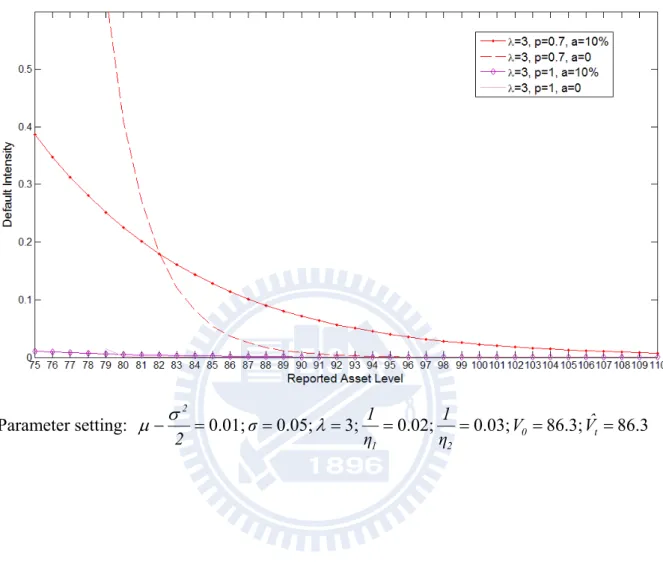
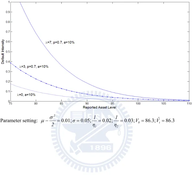
h h t, t t p lim 0 h t t H      . (14) Figure 4a illustrates the different between the default intensity of the modeled firm, the asset value of which has an asymmetric jump, with and without perfect information; besides, the special case of one-sided jump is also given. From this figure, we have three findings about the default intensity. First, the intensity with noise (a=10%) is less sensitive with reported asset level than the intensity without noise (a=0) as long as the jump is considered in the asset process. However, in the case that the value of asset follows a pure diffusion ( =0), the intensity with noise is always greater than the intensity without noise, which is zero at any reported asset level (Duffie and Singleton 2001). Second, if only the upward jump is included, the intensity is close to zero regardless of information quality. Third, at the same probability of upward jump, the intensity increases over the whole level of the reported asset as the arrival rate of jump increases, as illustrated in Figure 4b, whereas the intensity decreases for the low reported asset level but increase for the high reported asset level as information become more dubious, as illustrated in Figure 4a. It is suggested that there is a neutral point where the intensity is not affected.

From Figure 4c, it may be concluded that the arrival rate of jump creates greater impact on the intensity as the standard deviation of noise increases (a) from 0 to 25% at the reported

asset level (86) higher than the neutral point. In contrast, from Figure 4d, at the reported asset level (80) lower than the neutral point, the impact of jump initially increases as a increases from 0 to 5% and then decrease as a increases from 5% to 25%. In addition, the impact of noise on intensities will be saturated as the standard deviation of noise is large enough for both higher and lower reported asset level.

3.3 Credit Spreads

According to Kou and Wang(2004), under the risk-neutral probability measure , the return process given by



      _{  }      _{ }  Nt 1 i i t 2 t t W Y 2 1 r X    , 0X₀  . (15)

Where W_t is a standard Brownian motion under ,



_N ;_t0



t is a Poisson process with

intensity __{. The log jump size}





  

2 1 ,Y

Y still from a sequence of i.i.d. random variables

with a new double exponential density _{ } y _{y 0}

2 0 y y 1 Y (y) p e I q e I f 1 2                 The constants 1 0, 0; 1            _{, p ,q p q} 2 1   , and :

 

1 1        _  _    1 q 1 p e E 2 2 1 1 Y      . All sources of

randomness, N_t, W_t, and Ys, are still independent under .

For a given time to maturity T, the yield spread on a given zero-coupon bond sold at a price 0 is the real number  such that  T t

T , t    

 _e-r _{. We assume the bond holder}

at time t is given by   

_

_









T , t t t t r t T , t t t t r t t T T , t  1 h e E   he RE     _          _e-r ₍₁₆₎

where h_s is the conditional probability at time s under a risk-neutral probability measure  of default between s and s+1, given the information available at time s in the event of no default by s. Besides, r is the risk-free rate.

From Figure 5, it can be shown how the asymmetric jumps and noisy information create impacts on the term structure of credit spreads. First of all, noisy information tends to reshape the term structure from a hump to a monotone; in other words, the short spread will ascend and the long spread will descend while noise increases. This phenomenon results from the fact that the uncertainty causes the default probability having a more moderate variation with maturity, as illustrated in Figure 6. Secondly, as the arrival rate of jump increases, the term structure is still a humped-like curve, but the spread will be ascended over the whole range of maturity. Finally, the term structure of credit spreads is monotone if the both the asymmetric jump and the noisy information are simultaneously considered and large enough. The term structure of credit spreads therefore can be more enriched by including jumps and noise.

4 Conclusion

The pure diffusion approach for structural model with noisy information is generalized in this paper by including jumps in the firm-value processes. The explicit solution of the default

probability for this structural model is given, and numerical results show how the combination of the noisy information and the asymmetric jump brings the impacts on the credit risk.

Firstly, the opposite ways of impact of noise on the default intensity depends on whether the lower or higher range of the reported asset level is considered, and the noisy information will hence make the intensity with jump less sensitive with the reported asset level. Secondly, for the term structure of credit spread, the noisy information tends to reshape the term structure from a hump-like curve to a more flattened one; however, as the arrival rate of jump increases, the term structure is still hump-like, but the spread will be ascended over the whole range of maturity. Furthermore, it is found that the term structure of credit spreads is monotone if the two factors are simultaneously considered and large enough.

In short, the term structure of credit spreads is enriched by simultaneously incorporating the asymmetric jump and the noisy information into our credit risk model, and this generalization could be more potential to interpret empirical data in real world where rare events beyond the realm of normal expectations happen.

Reference

[1] Duffie, D., and K. Singleton. “Modeling Term Structures of Defaultable Bonds”, Reviews of Financial Studies, 12, 4, pp. 687-720, 1999.

[2] Duffie, D., K. Singleton. Credit Risk: Pricing, Measurement, and Management.

[3] Duffie, D., and D. Lando. “Term structures of credit spreads with incomplete accounting information”, Econometrica, 69, 3, pp. 633-664, May 2001.

[4] Guo, X., R. A. Jarrow, and Y. Zeng. “Credit Risk Models with Incomplete Information”, working paper, June 2008.

[5] John C. H.. Option, Futures, and other Derivatives. Pear.

[6] Kou, S. G.. “A Jump-Diffusion Model for Option Pricing”, Management Science, 48, 8, pp. 1086-1101, August 2002.

[7] Kou, S. G., and H. Wang. “First passage times for a jump diffusion process”, Adv. Appl. Probab, 35, pp. 504-531, 2003.

[8] Kou, S. G., and H. Wang. “Option pricing under a double exponential jump diffusion model”, Management Science, 50, 9, pp. 1178-1192, September 2004.

[9] Scherer, M.. “A structural Credit-Risk Model based on a Jump Diffusion”, working paper, December 2005.

[10] Schmid, B.. Credit Risk Pricing Models: Theory and Practice.

[12] Zhou, C.. “The term structure of credit spreads with jumps”, Journal of Banking and Finance, 1997

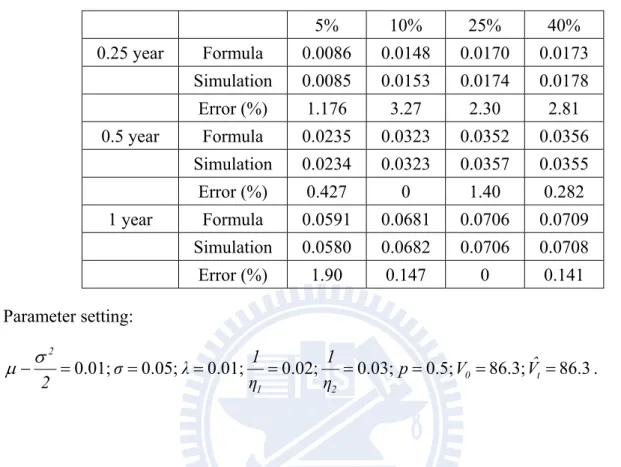
Table 1a: Comparison between Monte Carlo simulation and explicit solution of default probability. (λ=0.01). The simulation is based on 1,000,000 simulation runs.

5% 10% 25% 40% 0.25 year Formula 0.0086 0.0148 0.0170 0.0173 Simulation 0.0085 0.0153 0.0174 0.0178 Error (%) 1.176 3.27 2.30 2.81 0.5 year Formula 0.0235 0.0323 0.0352 0.0356 Simulation 0.0234 0.0323 0.0357 0.0355 Error (%) 0.427 0 1.40 0.282 1 year Formula 0.0591 0.0681 0.0706 0.0709 Simulation 0.0580 0.0682 0.0706 0.0708 Error (%) 1.90 0.147 0 0.141 Parameter setting: 86.3 86.3; 0.5; 0.03; 0.02; 0.01; 0.05; 0.01;          _{0 t} 2 1 2 Vˆ V p η 1 η 1 λ σ 2   .

Table 1b: Comparison between Monte Carlo simulation and explicit solution of default probability. (λ=3). The simulation is based on 1,000,000 simulation runs.

5% 10% 25% 40% 0.25 year Formula 0.0491 0.0584 0.0601 0.0602 Simulation 0.0483 0.0574 0.0598 0.0592 Error (%) 1.66 1.74 0.50 1.69 0.5 year Formula 0.1053 0.1131 0.1127 0.1124 Simulation 0.1027 0.1109 0.1091 0.1083 Error (%) 2.53 1.98 3.30 3.79 1 year Formula 0.2064 0.2061 0.2005 0.1994 Simulation 0.2033 0.2028 0.1958 0.1963 Error (%) 1.52 1.63 2.40 1.58 Parameter setting: 86.3 86.3; 0.5; 0.03; 0.02; 3; 0.05; 0.01;          _{0 t} 2 1 2 Vˆ V p η 1 η 1 λ σ 2   .

Figure 1: Probability of first passage time, for different arrival rate of jump and the probability of upward jump.

Parameter setting:  0.01; 0.05; 0.02; 0.03; ₀ 86.3; _t 86.3 2 1 2 Vˆ V η 1 η 1 σ 2   .

Figure 2a: Conditional density of V_t, for different standard deviation of noise. ( 0.01, p=0.5) Parameter setting: 86.3 86.3; 0.03; 0.02; 0.5; 0.01; 0.05; 0.01;          _{0 t} 2 1 2 Vˆ V η 1 η 1 p σ 2   

Figure 2b: Conditional density of V_t, for different standard deviation of noise. ( =3, p=0.5) Parameter setting: 86.3 86.3; 0.03; 0.02; 0.5; 3; 0.05; ; 0          _{0 t} 2 1 2 Vˆ V η 1 η 1 p σ 01 . 2   

Figure 2c: Conditional density of V_t, for different standard deviation of noise. ( =3, p=0.7) Parameter setting: 86.3 86.3; 0.03; 0.02; 0.7; 3; 0.05; 0.01;          _{0 t} 2 1 2 Vˆ V η 1 η 1 p σ 2    .

Figure 3: Default probability for time horizon 1 year, varying standard deviation of noise. Parameter setting:  0.01; 0.05; 0.02; 0.03; ₀ 86.3; _t 86.3 2 1 2 Vˆ V η 1 η 1 σ 2   .

Figure 4a: Default intensity, for different probabilities of upward jump, with noiseless and noisy information. Parameter setting:  0.01; 0.05; 3; 0.02; 0.03; ₀ 86.3; _t 86.3 2 1 2 Vˆ V η 1 η 1 σ 2   

Figure 4b: Default intensity, for different arrival rates of jump, with noisy information. Parameter setting:  0.01; 0.05; 0.02; 0.03; ₀ 86.3; _t 86.3 2 1 2 Vˆ V η 1 η 1 σ 2  

Figure 4c: Default intensity, for different arrival rates of jump and varying standard deviation of noise. (Vˆ_t 86) Parameter setting: 86 86.3; 0.03; 0.02; 0.7; 3; 0.05; 0.01;          _{0 t} 2 1 2 Vˆ V η 1 η 1 p σ 2    .

Figure 4d: Default intensity, for different arrival rates of jump and varying standard deviation of noise. (Vˆ_t 80) Parameter setting: 80 86.3; 0.03; 0.02; 0.7; 3; 0.05; 0.01;          _{0 t} 2 1 2 Vˆ V η 1 η 1 p σ 2    .

Figure 5: Credit Spread, for different arrival rates of jump, with noiseless and noisy information.

Parameter setting: 0.05; 0.05; 0.7; 0.02; 0.03; ₀ 86.3; _t 86.3 2 1 Vˆ V η 1 η 1 p σ r

Figure 6: The default probability, with noiseless and noisy information. Parameter setting: 0.05; 0.05; 3; 0.7; 0.02; 0.03; ₀ 86.3; _t 86.3 2 1 Vˆ V η 1 η 1 p σ r  .

Appendix

Appendix A. Notations

Notation 1: (for equation (4))

Note that to simplify the notation, we shall drop the superscript ′ in parameters, i.e., using



,  , p , q ,  , ₁  rather than ₂





,, p , q , ₁, ₂.





 

! n t e n N n t t n       





 

_

_





     _     _{   }  n 1 k k 1 1 1 k 1 k , n mn 1 n n 2 t mn 2 1 , t t 1 , ; t x I t P t 2 e lim , , q , p , L 2 1            





 

_

_





      _     _{ }  n 1 k k 1 2 2 k 2 k , n 2 n n 2 t mn 2 1 , t t 1 , ; t x I t Q t 2 e lim , , q , p , M 2 2             1 n k 1 , q p i n k i 1 k n P i n i i n 2 1 2 1 n k i k i 2 1 1 k , n                                       



_ _{ } _ 1 n k 1 , q p i n k i 1 k n Q n i i k i 2 1 2 1 n k i i n 2 1 1 k , n                                       



_ _{ } _ 1 0 0 , q Q , p P n n , n n n , n        













                 _{ }                         _{  }                





        1 n , 0 , 0 , c e 2 c Hh e 1 n , 0 , 0 , c e 2 c Hh e , , ; c I n 0 i 2 1 n i i n c n 0 i 2 1 n i i n c n 2 2 2 2                                              .  , 2 , 1 , 0 n , 0 dt e ) x t ( ! n 1 dy ) y ( Hh ) x ( Hh x 2 t n x n 1 n 2     



 _



 

Note that to compute the Hh function, the three-term recursion of Hh which is 1 ,   Hh_ (x) xHh_ (x) n ) x ( nHh_{n n 2 n 1} should be used.

Notation 2: (for equation (5))





                     1, b 2, , 1 , 2 1 , 2 b , 1 , 2 , 1 1 2 1, ,b e e , q , p , A        







_



_





  



              b 1, b 2, , 1 , 2 1 1 , 2 , 1 1 2 1, ,b e e , q , p , B       





_

   _    _{ }  mn 0 n 0 n mnlim n!H h, , ;n x , b , C      _





_





_

  



       _       mn 1 n n 1 j 1 j 0 k k k 1 j , n j , n n mn 2 1 AP BP H h, ,c ;n ! n lim x , b , , , q , p , D      _





_

    



      mn 1 n n 0 j j j 1 n mn 2 1 H h, ,c ;n ! n p lim B x , b , , , q , p , E      _





_





_

  



       _        mn 1 n n 1 j 1 j 0 k k k 2 j , n j , n n mn 2 1 AQ BQ H h, ,c ;n ! n lim x , b , , , q , p , F      _ 1 n i 1 , q p j n i j 1 i n P j n j j n 2 1 2 i j 2 1 1 1 n i j i, n                                               



_ _{ }_ 1 n i 1 , p q j n i j 1 i n Q j n j j n 2 1 1 1 n i j i j 2 1 2 k , n                                               



__{ }_ n n , n n n , n p ,Q q P while                         x b h , 2 , c , c n i 1 , i j i n p q j n Q 1 n i 2 , P P , Q P 2 2 2 1 1 j n 2 1 1 1 n i j i j 2 1 2 j n j k , n 1 k , n k , n i 2 1 2 1 n 1 i i, n 1 , n                                                                    









dt, i 1, n 0 t a t c Hh t e 2 1 n ; c , b , a H 2 _i i n 0 t b c 2 1 i 2          _         _

















H



a,b,c;n



i a 1 n ; c , b , a H i c 1 n ; c , b , a H i 1 n ; c , b , a H_i  _i2   _i1   _i1 should be used..

Appendix B. Derivation of the cumulative distribution of

Z_t

,





Z_t  z



Suppose



₁,₂,_



is a sequence of i.i.d. exponential random variables with rate  0, V and U are random variables with normal distribution _N



_{0, }2



_{and N}



_,a2



_{respectively.}

Let



2



t tV U ~N ,

H     and _2 _2_ta2_{. Then for every n1,}

(1) The density functions are given by

 

 

 

     _{  }       _                s Hh e 2 e s f 2 n s _{n 1} H 2 n 1 i i t

 

 

 

      _{ }      _                s Hh e 2 e s f 2 n s _{n 1} H 2 n 1 i i t

(2) The tail probabilities are given by





 

 

      _{   }     _   _                , 1 , ; x I 2 e x H n 2 n _{n 1} 1 i i t 2





 

 

      _{ }     _   _                , 1 , ; x I 2 e x H n 2 n _{n 1} 1 i i t 2 Proof.

(1) The density functions of Htin1i and Ht ni1i:

 

_





  

  _ s  f_ sh f h dh f _H H n i i n i i t ₁ ₁















        _     s n s h n h _dh n h s e e ₂ 2 1 2 exp 2 1 ! 1       



















        _{   }    s n s n _{h h dh} n h s e 2 2 2 2 1 2 2 1 exp 2 1 ! 1         













  





        _{    }    s n s n _{h dh} n h s e             2 2 2 2 2 2 1 2 2 1 exp 2 1 ! 1  

_

_











         _{  }    s n s n _{h dh} n h s e e 2 2 2 1 2 2 1 exp 2 1 ! 1 2           Letting y



h 2



h y_{ }2_{ }, dh _dy      _{   }   , , yields that

 

 



_

_



 





       _{  }                _{  }                                 





                                                    s Hh e ) ( 2 e dy 2 y exp 2 1 ! 1 n y s e ) ( e dy 2 y exp 2 1 ! 1 n y s e e s f 1 n s n 2 s 2 1 n 2 1 n n s s ₂ n 1 2 2 n s H 2 2 2 n 1 i i t here









2 dy Hh

 

s y exp 1 n y s 1 n s n 1 2               



_! . Similarly,

 



  

















                       s 2 2 1 n h n s H H dh 2 h exp 2 1 1 n s h e e dh h f s h f s f n 1 i i n 1 i i t          ! Let h=-h,

 



_



_





















  



 

_

_















                   _{  }          _{    }          _{    }      s ₂ 2 2 1 n 2 n s s ₂ 2 ₂ 2 ₂ 2 1 n n s s _{2 2 2} 2 1 n n s H dh h 2 1 exp 2 1 1 n h s e e dh 2 h 2 1 exp 2 1 1 n h s e dh h 2 h 2 1 exp 2 1 1 n h s e s f 2 n 1 i i t                                    ! ! !





_{, yields} Letting y h 2 h y_{ }2_{ }, dh _dy      _{   }  

 

 



_

_



 





        _{ }               _{   }                                 





                                                    s Hh e ) ( 2 e dy 2 y exp 2 1 1 n y s e ) ( e dy 2 y exp 2 1 1 n y s e e s f 1 n s n 2 s 2 1 n 2 1 n n s s 2 n 1 2 2 n s H 2 2 2 n 1 i i t ! ! (2)



H x





H n x



1 i i t n 1 i i t        . and





 

 

 

 

      _{   }       _{  }           



                              , 1 , ; x I 2 e ds s Hh e 2 e x H 1 n n 2 x n 1 s n 2 n 1 i i t 2 2 where 



   c n x n(c; , , ) e Hh( x )dx, n 0 I       . Similarly,





 

 

 

 

      _{ }        _{ }          



                              , 1 , ; x I 2 e ds s Hh e 2 e x H 1 n n 2 x n 1 s n 2 n 1 i i t 2 2 Therefore,





_                   





   z Y U W t 2 z Z n 1 j j t t 2 0 n n t                         





   z Y H t 2 n 1 j j t 2 0 n n                     t H z 2 t 2 0                     







     z H t 2 P n 1 j t 2 n 1 k n,k 0 n n j     

                







     z H t 2 Q n 1 j t 2 n 1 k n,k 0 n n j                                   t 2 z 2 0  

 





                        n 1 k 1 1 2 1 k k 1 k , n 0 n n 2 1 , 1 , ; t 2 z I P 2 e 1 2 1                   









                      n 1 k 2 2 2 1 k k 2 k , n 0 n n 2 1 , 1 , ; t 2 z I Q 2 e 2 2 2                  Let





 





_

_

 





                                                  n 1 k 2 2 2 1 k k 2 k , n 0 n n 2 1 n 1 k 1 1 2 1 k k 1 k , n 0 n n 2 1 , 1 , ; t 2 z I Q , , q , p , M , 1 , ; t 2 z I P , , q , p , L                             Then,





 





 



1 2



2 1 2 1 2 1 2 0 n 1 j j t t 2 0 n n t , , q , p , M 2 e , , q , p , L 2 e t 2 z z Y U W t 2 z Z 2 2 2 1 2 1                                                                                 



