行政院國家科學委員會專題研究計畫 成果報告
利用 preimage 分析萃取規則之實作
研究成果報告(精簡版)
計 畫 類 別 : 個別型 計 畫 編 號 : NSC 97-2410-H-004-117- 執 行 期 間 : 97 年 08 月 01 日至 98 年 07 月 31 日 執 行 單 位 : 國立政治大學資訊管理學系 計 畫 主 持 人 : 蔡瑞煌 計畫參與人員: 學士級-專任助理人員:沈軒豪 報 告 附 件 : 出席國際會議研究心得報告及發表論文 處 理 方 式 : 本計畫可公開查詢中 華 民 國 98 年 07 月 17 日
行政院國家科學委員會補助專題研究計畫
■ 成 果 報 告
□期中進度報告
利用 preimage 分析萃取規則之實作
計畫類別:■ 個別型計畫 □ 整合型計畫
計畫編號:NSC 97-2410-H-004-017-
執行期間: 97 年 8 月 1 日至 98 年 7 月 31 日
計畫主持人:蔡瑞煌
共同主持人:
計畫參與人員: 沈軒豪
成果報告類型(依經費核定清單規定繳交):■精簡報告 □完整報告
本成果報告包括以下應繳交之附件:
□赴國外出差或研習心得報告一份
□赴大陸地區出差或研習心得報告一份
■出席國際學術會議心得報告及發表之論文各一份
□國際合作研究計畫國外研究報告書一份
處理方式:除產學合作研究計畫、提升產業技術及人才培育研究計畫、
列管計畫及下列情形者外,得立即公開查詢
□涉及專利或其他智慧財產權,□一年□二年後可公開查詢
執行單位:國立政治大學資訊管理學系
中 華 民 國 98 年 7 月 15 日
報告內容
ARTIFICIALNEURALNETWORKSASAFEATUREDISCOVERYTOOL
This study proposes the preimage analysis and its associated belief justification process
regarding the application of continuous-valued single-hidden layer feed-forward neural
network (SLFN) to discovering features – certain relationships between explanatory (input) and
observed (output) variables – embedded in the (training) data. The preimage analysis explicitly
specifies the preimage of network and discloses its preimage-related properties. The preimage
of a given output of an SLFN is the collection of all inputs each of that generates the output.
The seminal publication of (Rumelhart & McClelland, 1986) states that Artificial Neural
Networks (ANN) can be trained primarily through examples; ANN can do the general
pattern-recognition; and ANN can learn general rules of optimal behavior. Since then, these
claims stimulate studies in many fields to develop various ANNs as modeling tools to check the
validity of the claims. Lots of experimental results are positive. For instance, Sgroi & Zizzo
(2007) state that ANNs “are consistent with observed laboratory play in two very important
senses. Firstly, they select a rule for behavior which appears very similar to that used by
laboratory subjects. Secondly, using this rule they perform optimally only approximately 60%
Results of these researches infer that well-trained ANNs possess features embedded in
(training) data. Thus, some practitioners may go one step further to conduct researches that
address the issue of extracting features embedded in data from well-trained ANNs. For instance,
based upon the empirical data, one wants to identify the relative influence of factors for pricing
newly issued securities. The practitioner first gets several well-trained networks and then from
these networks extracts certain features. The rule (1) is one of such feature examples. Hopefully,
the extracted rules could depict features embedded in data and could help identify the
significant factor.
Rule: If the input sample is in some sub-region of the input space, then the predicted price
value is given by a corresponding linear regression equation. (1)
Note that the feature-discovery practitioner (and researcher) may be merely interested in any
(ANN or statistical) tool that can help analyze the data to discover something interesting or
significant, instead of in the interaction of human cerebral activities and its explanation that
results in the fundamentals of ANN. Regardless, the task faced by a feature-discovery
practitioner is not easier because ANN simply behaves as a black box, i.e., a system that
produces “certain outputs from certain inputs without explaining why or how” (Rabuñal,
Dorado, Pazos, Pereira, & Rivero, 2004). Nevertheless, ANN researchers have spent substantial
from trained ANNs (rule extraction), and utilize ANNs to refine existing rule bases (rule
refinement).” (Andrews, Diederich, & Tickle, 1995, page 373) Some, but not exhaustive,
studies for these purposes are presented in (Andrews, Diederich, & Tickle, 1995; Setiono & Liu,
1997; Tickle, Andrews, Golea & Diederich, 1998; Tsaih, Hsu, & Lai, 1998; Taha & Ghosh,
1999; Zhou, Chen, & Chen, 2000; Saito & Nakano, 2002; Setiono, Leow, & Zurada, 2002;
Baesens, Setiono, Mues, & Vanthienen, 2003)
Despite these studies, the black box nature of ANN persists and any feature-discovery
intention is better to cope with following issues. First, the approach should disclose true
properties from ANN. Most of above studies do not seem to generalize to the situation since
they are contrived to explore restrictedly with limited data such that the extracted rules are
dubious and unlikely to be considered as patterns of knowledge embedded in data. Consider the
rule stated in (1). To spot its premise, most works use either training data or generated data,
which the trained network itself yields. Such an approach is data sensitive and requires
extensive amount of data to be accurate. The limited number of (training or generated) data
instances leads to a suspicion of the generalization of rule (1) in interpolating and extrapolating
any unexplored data values.
Second, since features learned by an ANN distribute over the entire network as weight values,
simultaneously investigate several kinds of features to get a better understanding about the
(training) data. The above studies do not seem to generalize to the situation, since they base
upon predefined schemes like rule (1) for extracting rules.
Third, it is possible to have a sub-perfect learning result since, in most studies (e.g., financial
market tests), it is characteristically more difficult to determine the best architecture of SLFN.
Besides, noises in the training samples prevent networks from perfect fittings. The possibility
of a sub-perfect learning result leads to a conservative attitude on embracing the obtained
preimage-related properties. The practitioner with such understanding has conservatism in the
straightforward feature acquisition. The above studies do not seem to cope with such
conservatism.
Fourth, the practitioner normally has some personal beliefs when he conducts the
feature-discovery experiment. Any such belief, if available, is in the form of tacit knowledge
about the relationship between the explanatory and observed variables. However, to draw
parallels between the beliefs and the observed features needs professional interpretations due to
the tacit nature of the former and the complex nature of the latter. That is, the practitioner has to
contrast the similarities and differences between beliefs and observed featuresand then to infer
properly. Even if the beliefs and observed features suggest different views, the practitioner may
justification is a kind of knowledge internalization stated by Nonaka & Takeuchi (1995). The
above studies do not seem to provide such discussions.
This study addresses these issues. Specifically, for feature discovery via well-trained SLFNs,
this study proposes the preimage analysis that explicitly specifies the preimage of network to
disclose its preimage-related properties. For complex preimage-related properties, this study
then proposes the following belief justification process, in which the practitioner’s (prior)
beliefs are refined based upon the examination results of preimage-related properties. The
beliefs lead to propositions of the experiment. Based upon the propositions, the practitioner
first picks up relevant explanatory and observed variables and collects the sample accordingly.
Then he trains SLFNs and, after the training, applies the preimage analysis to the selected
SLFNs. For each belief, the practitioner inspects relevant preimage-related properties. Such
inspection leads to a belief justification process. If there is no such prior belief, the rule (2) and
the observed preimage-related properties exclusively make statements about features embedded
in data.
Research findings of this study are summarized as follows:
(I) the preimage analysis is not data intensive and the inspected preimage-related properties
(III) the inspected preimage-related properties provide further insights about rule (2) and thus
about features embedded in data. In rule (2), x is the vector of explanatory variables; y is
the network’s response; f: X → Y is the function of the SLFN and y ≡ f(x); y’ is a constant; and the preimage f -1 is the inverse function of f.
Rule: If (x ∈ the f -1(y’) region), then (y = y’). (2)
(IV) several kinds of features can be simultaneously investigated through inspecting
preimage-related properties.
The remainder of this paper is organized as follows. Section II starts with the list of notations
used in the study and then gives the proposed preimage analysis. From the preimage analysis,
we find that rank(WH) determines characteristics of the preimage-related properties, in which
WH is the matrix of weights between the input variables and the hidden nodes and rank(D) is
the rank of matrix D. Hereafter, SLFN-p denotes an SLFN whose rank(WH) equals p. Section
III shows the application of preimage analysis to the two SLFN-1 network solutions of the 3-bit
parity problem. Some implications regarding the feature-discovery application via SLFN-1
networks are offered in Section VI. It is readily seen that the preimage-related properties of
SLFN-1 are easy to understand. However, learning algorithms adopted in most studies likely
result in SLFN-p networks with p ≥ 2 and these SLFN networks own complex preimages and
illustrated through the feature-discovery application to the bond pricing experiment, which
releases an SLFN-3 network.Some further discussions and future work are presented at the end.
THEPROPOSEDPREIMAGEANALYSIS
List of notations used in mathematical representations: Characters in bold represent column
vectors, matrices or sets; (⋅)T denotes the transpose of (⋅).
I ≡ the amount of input nodes;
J ≡ the amount of hidden nodes;
x ≡ (x1, x2, …, xI)T: the input vector, in which xi is the ith input component, with i from 1
to I;
a ≡ (a1, a2, …, aJ)T: the hidden activation vector, in which aj is the activation value of
the jth hidden node, with j from 1 to J;
y ≡ the activation value of the output node and y = f(x) with f being the function mapping x to y;
H ji
w ≡ the weight between the ith input variable and the jth hidden node, in which the superscript H throughout the paper refers to quantities related to the hidden layer;
H j w ≡ (wHj1, H j w 2, …,wHjI)T; WH ≡ ( H 1 w , H 2 w , …, H J
w )T, the J×I matrix of weights between the input variables and the
hidden nodes;
H j
O j
w ≡ the weight between the jth hidden node and the output node, in which the
superscript O throughout the paper refers to quantities related to the output layer;
wO ≡ ( O w1 , O w2 , …, O J w )T; and O
w0 ≡ the bias value of the output node.
Without any loss of generality, assume the tanh activation function is adopted in all hidden
nodes. Denote the collection of H j
w0, wHj , wO
,and w0O by θ. Given θ, the resulting f of SLFN is
the composite of the following mappings: the activation mapping ΦA : ℜI → (-1, 1)J that maps
an input x to an activation value a (i.e., a = ΦA(x)); and the output mapping ΦO : (-1, 1)J → (w0O
-
∑
= J j O j w 1 , O w0 +∑
= J j O j w 1) that maps an activation value a to an output y (i.e., y = ΦO(a)). Note that,
since the range of ΦA and the domain of ΦO are set as (-1, 1)J, the range in the output space ℑ ≡
( O w0 -
∑
= J j O j w 1 , O w0 +∑
= J j O j w 1) contains all achievable output values. For ease of reference in later
discussion, we also call RI the input space and (-1, 1)J the activation space.
Thus, f -1(y) ≡ ΦA-1(ΦO-1(y)) with
ΦO-1(y) ≡ {a ∈ (-1, 1)J|
∑
= J j j O ja w 1 = y - O w0 }, (3) ΦA-1(a) ≡
J j 1= {x ∈ ℜI|∑
= I i j H jix w 1 = tanh-1(aj) -wHj0}, (4) where tanh-1(x) ≡( )
-x x 1 1 ln 5 .0 + . Formally, the followings are defined for every given θ:
(a) A value y ∈ ℜ is void if y ∉ f({ℜI}), i.e., for all x ∈ ℜI, f(x) ≠ y. Otherwise, y is non-void.
(b) A point a ∈ (-1, 1)J is void if a ∉ ΦA({ℜI}), i.e., for all x ∈ ℜI, ΦA(x) ≠ a. Otherwise, a is non-void. The
(c) The image of an input x ∈ ℜI is y ≡ f(x) for y ∈ ℑ.
(d) The preimage of a non-void output value y is f -1(y) ≡ {x ∈ ℜI| f(x) = y}. The preimage of a
void value y is the empty set.
(e) The internal-preimage of a non-void output value y is the intersection of ΦO-1(y) and the
non-void set on the activation space.
Given θ, the preimage analysis is conducted in the following four steps to specify the preimage:
Step 1: Derive the expression of ΦO-1(y);
Step 2: Derive the expression of the non-void set;
Step 3: Derive the expression of internal-preimage of a non-void output value y; and
Step 4: Derive the expression of preimage f -1(y).
From eqt. (3), with the given θ, ΦO-1(y) is a hyperplane in the activation space. As y changes,
ΦO-1(y) forms parallel hyperplanes in the activation space; for any change of the same
magnitude in y, the corresponding hyperplanes are spaced by the same distance. The activation
space is entirely covered by these parallel ΦO-1(y) hyperplanes, orderly in terms of the values of
y. These parallel hyperplanes form a (linear) scalar field (Tsaih, 1998). That is, for each point a of the activation space, there is only one output value y whose ΦO-1(y) hyperplane passes point
From eqt. (4), ΦA-1(a) is a separable function such that each of its components lies along a
dimension of the activation space. Moreover, ΦAj-1(aj) ≡{x ∈ ℜI|
∑
= I i j H jix w 1 = tanh-1(aj) -wHj0} is a
monotone bijection that defines a one-to-one mapping between the activation value aj and the
input x. For each aj value, ΦAj-1(aj) defines an activation hyperplane in the input space.
Activation hyperplanes associated with all possible aj values are parallel and form a (linear)
scalar activation field in the input space. That is, for each point x of the input space, there is
only one activation value aj whose ΦAj-1(aj) hyperplane passes point x; all points on the ΦAj-1(aj)
hyperplane are associated with the activation value aj. Each hidden node gives rise to an
activation field, and J hidden nodes set up J independent activation fields in the input space.
Thus, with the given θ, the preimage of an activation value a by ΦA-1 is the intersection of J
specific hyperplanes. The intersection
J j 1= {x ∈ ℜI|∑
= I i j H jix w 1= tanh-1(aj) -wHj0} can be represented as {x| W
H
x = ω(a)}, where ωj(aj) ≡ tanh-1(aj) -wHj0 for all 1 ≤ j ≤ J, and ω(a) ≡ (ω1(a1), ω2(a2),…, ωJ(aJ))
T
.
Given θ and an arbitrary point a, ω(a) is simply a J-dimensional vector of known component values and the conditions that relates a with x can be represented as
WHx = ω(a), (5)
which is a system of J simultaneous linear equations with I unknowns.
Let rank(D) be the rank of matrix D and (D1D2) be the augmented matrix of two matrices
equations if rank(WHω(a)) = rank(WH) + 1 (c.f. (Murty, 1983)). In this case, the corresponding point a is void. Otherwise, a is non-void. Note that, for a non-void a, the
solution of eqt. (5) defines an affine space of dimension I - rank(WH) in the input space. The
discussion establishes Lemma 1 below.
Lemma 1: (a) An activation point a in the activation space is non-void if its corresponding
rank(WHω(a)) equals rank(WH). (b) The set of input values x mapped onto a non-void a forms an affine space of dimension I - rank(WH) in the input space.
By definition, the non-void set equals {a ∈ (-1, 1)J
| aj = tanh(
∑
= I i j H jix w 1 + H j w0) for 1 ≤ j ≤ J, x ∈ ℜI}.Check that WH is a J×I matrix. If rank(WH) = J, Lemma 1 says that no activation point a can be void and leads to Lemma 2 below. For rank(WH) < J, Lemma 3 characterizes the non-void set,
which requires the concept of manifold. A p-manifold is a Hausdorff space X with a countable
basis such that each point x of X has a neighborhood that is homomorphic with an open subset
of ℜp (Munkres, 1975). A 1-manifold is often called a curve, and a 2-manifold is called a
surface. For our purpose, it suffices to consider Euclidean spaces, the most common members
of the family of Hausdorff spaces.
Lemma 2: If rank(WH) equals J, then the non-void set covers the entire activation space.
Lemma 3: If rank(WH) is less than J, then the non-void set in the activation space is a
A(y), the intersection of ΦO-1(y) and the non-void set in the activation space, is the
internal-preimage of y. Mathematically, for each non-void y, A(y) ≡ {a|rank(WH ω(a)) = rank(WH), a∈ ΦO-1(y)}. Consider first rank(WH) = J. In this case, Lemma 2 says that the
non-void set is the entire activation space. Thus, A(y) equals ΦO-1(y). If rank(WH) < J, then A(y)
is a subset of ΦO-1(y). Thus, we have the following Lemma 4. Furthermore, A(y)’s are aligned
orderly according to ΦO-1(y) and all non-empty A(y)’s form an internal-preimage field in the
activation space. That is, there is one and only one y such that a non-void a ∈ A(y); and for any a on A(y), its output value is equal to y.
Lemma 4. For each non-void output value y, all points in the set A(y) are at the same
hyperplane.
Now the preimage of any non-void output value y, f -1(y), equals {x ∈ ℜI| WHx = ω(a) with all a ∈ A(y)}. If rank(WH
) = J, then, from Lemma 2 and Lemma 1(b), the preimage f -1(y) is a
(I-1)-manifold in the input space. For rank(WH) < J, from Lemma 3 and Lemma 1(b),
1. if rank(WH) = 1 and A(y) is a single point, then f -1(y) is a single hyperplane;
2. if rank(WH) = 1 and A(y) consists of several points, then f -1(y) may consist of several
disjoint hyperplanes;
3. if 1 < rank(WH) < J and A(y) is a single (rank(WH)-1)-manifold, then f -1(y) is a single
(I-1)-manifold; and
f -1(y) consists of several disjoint (I-1)-manifolds.
Table 1 summarizes the relationship between the internal-preimage A(y) and the preimage f -1(y)
of a non-void output value y.
Table 1. The relationship between the internal-preimage A(y) and the preimage f -1(y) of a
non-void output value y.
The nature of A(y) A single intersection-segment
Multiple disjoint intersection-segments The nature of f -1(y) A single (I-1)-manifold Multiple disjoint (I-1)-manifolds
The input space is entirely covered by a grouping of preimage manifolds that forms a
preimage field. That is, there is one and only one preimage manifold passing through each x;
and the corresponding output value is the y value associated with this preimage manifold. Note
that the preimage manifolds are aligned orderly because A(y)’s are aligned orderly according to
ΦO-1(y)’s and the mapping of ΦA-1 is a monotone bijection that defines a one-to-one mapping
between an activation vector and an affine space.
Notice that rank(WH) determines the characteristic of the non-void set and thus the
characteristic of internal-preimage. For a SLFN-1 network, we can assume H j
w ≡ αjw for all j,
in which w is a non-zero vector and αjs are constants; as for a SLFN-p network with p > 1, we
can assume that vectors in the set of { H
1
w , H
2
w , …, H
p
w } are linearly independent and H j w ≡
∑
= P k H k jk 1 w γ for all j > p.APPLICATIONTOSOMEEXAMPLESOFSLFN-1NETWORK
In this section, we show the application of the preimage analysis to the following two kinds of
SLFN-1 network solutions of the 3-bit parity problem, in which the target output is 1 if the
input vector contains an odd number of -1s and -1 otherwise: (1) the SLFN network solution
with seven effective hidden nodes shown in Table 2, constructed by Huang & Babri (1998), and
(2) the SLFN network solution with two hidden nodes shown in Table 3.
Tab le 2. An SLFN network solution of the 3-bit parity problem constructed by Huang & Babri (1998), in which O w0 = 0.0 and w = (0.4, 0.5, 0.7)T. j wOj H j w 0 H j w 1 -239.9515868 0.651132681 0.0 w 2 65.96703854 0.283261412 -0.459839086 w 3 15.8645681 -0.452481126 -1.839356344 w 4 -369.5491494 0.467197046 -0.919678172 w 5 465.7997072 0.835068315 -0.919678172 w 6 -45.18900519 1.202939584 -0.919678172 w 7 -110.3929208 2.122617756 -1.839356344 w 8 128.6377379 1.386875218 -0.459839086 w
Tab le 3. An SLFN network solution of the 3-bit parity problem, in which O
w0 = 0.0 and w = (1, 1, 1)T.
j wOj H j w 0 H j w 1 18.58899737 0.0 0.4 w 2 -30.7174688 0.0 0.2 w
For the SLFN-1 network with µ ≡ 0.4x1+0.5x2+0.7x3 shown in Table 2, the preimage analysis
states that its non-void set equals {a ∈ (-1, 1)8| a1 = tanh(0.651132681), a2 =
tanh(0.283261412-0.459839086µ), a3 = tanh(-0.452481126-1.839356344µ), a4 =
tanh(0.467197046-0.919678172µ), a5 = tanh(0.835068315-0.919678172µ), a6 =
tanh(1.202939584-0.919678172µ), a7 = tanh(2.122617756-1.839356344µ), a8 =
tanh(1.386875218-0.459839086µ), µ ∈ ℜ}, which is an 1-manifold in (-1, 1)8; A(y) equals {a ∈ (-1, 1)8| a1 = tanh(0.651132681), a2 = tanh(0.283261412-0.459839086µ), a3 =
tanh(-0.452481126-1.839356344µ), a4 = tanh(0.467197046-0.919678172µ), a5 =
tanh(0.835068315-0.919678172µ), a6 = tanh(1.202939584-0.919678172µ), a7 =
tanh(2.122617756-1.839356344µ), a8 = tanh(1.386875218-0.459839086µ), 65.96703854 a2 +
15.8645681 a3 - 369.5491494 a4 + 465.7997072 a5 - 45.18900519 a6 - 110.3929208 a7 +
128.6377379 a8 = y +239.9515868 tanh(0.651132681), µ ∈ ℜ}, which may consist of one or
several 1-manifold segments in (-1, 1)8; and f -1(y) equals {x ∈ ℜ3| 0.4x1+0.5x2+0.7x3 = µ,
110.3929208tanh(2.122617756-1.839356344µ) + 128.6377379 tanh(1.386875218- 0.459839086µ) = y +239.9515868 tanh(0.651132681), µ ∈ ℜ}, which may consist of one or several 2-manifold segments in ℜ3
.
For the SLFN-1 network with µ ≡ x1+x2+x3 shown in Table 3, the preimage analysis states
that its non-void set equals {a ∈ (-1, 1)2| a1 = tanh(0.4µ), a2 = tanh(0.2µ), µ ∈ ℜ}, which is an
1-manifold in (-1, 1)2; A(y) equals {a ∈ (-1, 1)2| a1 =tanh(0.4µ), a2 =tanh(0.2µ), 18.58899737 a1-
30.7174688a2= y, µ ∈ ℜ}, which may consist of one or several 1-manifold segments in (-1, 1)
2
;
and f -1(y) equals {x ∈ ℜ3| x1+x2+x3 = µ, 18.58899737tanh(0.4µ) - 30.7174688tanh(0.2µ) = y, µ ∈
ℜ}, which may consist of one or several 2-manifold segments in ℜ3
.
Fig. 1 shows the relationship between the value of µ and the output value y, regarding the SLFN-1 networks shown in Table 2 and Table 3. The relationship between the preimage f -1(y)
and the output value y of these two SLFN-1 networks can be observed from Fig. 1. The y-µ graph also indicates the generalization of these two SLFN-1 networks.
Figure 1: The relationship between the value of µ and the output value y, regarding the SLFN-1 networks shown in Table 2 and Table 3.
IMPLICATIONSOFTHEFEATURE-DISCOVERYAPPLICATIONOFTHESLFN-1
NETWORKS
In general, for any SLFN-1 network with µ ≡ wT
x and H j
w ≡ αjw for all j, the preimage analysis
states that its non-void set equals {a ∈ (-1, 1)J| aj = tanh(αj µ +wHj0) ∀ j, µ ∈ ℜ}, which is an
1-manifold in (-1, 1)J; A(y) equals {a ∈ (-1, 1)J|
∑
= J j O j w 1 tanh(αj µ +wHj0) = y -O w0 , aj =tanh(αj µ +wHj0)
∀ j, µ ∈ ℜ}, which may consist of one or several 1-manifold segments in (-1, 1)J; and f -1(y) equals {x ∈ ℜI | wTx = µ,
∑
= J j O j w 1 tanh(αj µ +wHj0) = y -O w0 , aj = tanh(αj µ +wHj0) ∀ j, µ ∈ ℜ}, whichmay consist of one or several (I-1)-manifold segments in ℜI. These establish the following
H -4 -3 -2 -1 0 1 2 3 4 -5 -4 -3 -2 -1 0 1 2 3 4 5 SLFN-1 network shown in Table 2 SLFN-1 network shown in Table 3
orientation of the activation hyperplane in the input space corresponding to the jth hidden node.
Thus, we have Lemma 6.
Lemma 5: For SLFN-1, the preimage field is formed from a collection of preimage hyperplanes.
Lemma 6: For SLFN-1, the activation hyperplanes in the input space corresponding to all
hidden nodes are parallel, and the preimage hyperplane is parallel with the activation
hyperplane.
Outcomes of the preimage analysis lead to an understanding of the SLFN-1 itself and further
provides the following four insights about the usage of network and about the patterns
embedded in (training) data. First, SLFN-1 networks possess the hyperplane-preimage property,
which is their generalization. Therefore, the SLFN-1 should be used in the experiments desiring
a hyperplane-preimage relationship.
Second, the act to adopt the SLFN-1 architecture at the learning stage does already set the
hyperplane-preimage assumption and insert such feature into network. Third, when one gets a
SLFN-1 from training, he/she can infer that the empirical data bear the hyperplane-preimage
relationship. Fourth, the hyperplane-preimage relationship states that the observed variable of
interest is a function of a certain factor obtained from some linear combination of explanatory
variables. With such an insight, the practitioner may adopt a common regression method or
other suitable tool for data analysis after he/she has properly transformed the explanatory
application problem.
THEBONDPRICINGEXPERIMENT
In this section, we illustrate the feature-discovery process of a practitioner, who knows
bond-pricing mechanism well (but less than perfectly). Because bond pricing has been
well-studied in the literature, the purpose of this experiment is to illustrate the belief
justification process, not to discover extra features of bond pricing.
Before conducting the experiment, the practitioner has some personal beliefs and
propositions of the experiment. Based upon the propositions, he first picks up relevant
explanatory and observed variables and collects the sample accordingly. Below are the details
of his experimental design.
Let the theoretical bond price pc at time c is derived from (11), which serves as an example of
knowledge regarding the data.
∑ + + + ≡ = − − 0 0 1 , ) 1 ( ) 1 ( T k c k c c T c c r F r FR p (11)
where rc is the market rate of interest at time c; F = 100 is the face value of the bond; T0 is the
term to maturity at time c = 0; R is the coupon rate; and FR is the periodic coupon payment.
Then garbled bond prices yc are generated and used to simulate the set of data that may be
and variance (0.2)2, for all time c and bonds.
As depicted in Table 4, there are 18 hypothetical combinations of term to maturity and
contractual interest rate and generate a set of price data with c = 1/80, 2/80, …, 80/80 through
(11). The rate rc is derived from a normal random number generator of N(2%, (0.1%)2). Accordingly, there are 1,440 training samples with input variables Tc, R and rc, and the desired
output variable yc, where Tc ≡ (T0 - c) is the term to maturity at time c.
To examine the generalization of trained networks, the practitioner also generates 1,440 test
samples by similar means, except that T0, c, R and rc are randomly and independently generated
from {1, 2, …, 20} with a probability of 1/20 for each, {1/80, 2/80, …, 80/80} with a
probability of 1/80 for each, [0.0%, 3.0%] with a probability density function f(R) = 1/0.03, and
N(2%, (0.1%)2
), respectively. This setting results in varying instances among the test samples.
The Back Propagation learning algorithm of Rumelhart et al. (1986) is used to train 1,000
SLFNs, each of which has 4 hidden nodes and random initial weights and biases. Among these
1,000 SLFNs, the practitioner picks the three with the smallest mean square error (hereafter,
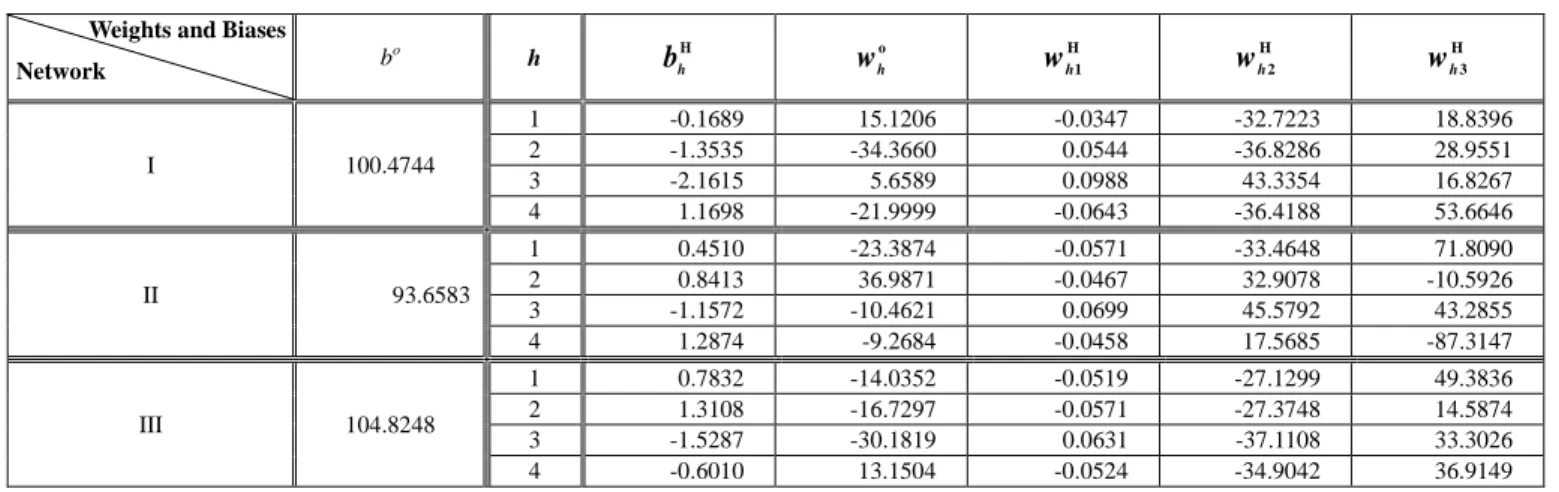
MSE) for the test samples. Table 5 shows the (final) weights and biases of these three networks,
hereafter named network I, II and III, respectively. The corresponding MSEs for the training
samples are 0.414, 0.404 and 0.451, respectively, and the corresponding MSEs for the test
samples are 0.429, 0.432 and 0.445, respectively. The average absolute deviation is
rank(WH) of all networks I, II and III are 3.
Take network I to illustrate the result of applying the preimage analysis to these three
networks. ΦO-1(y) = {a| 15.1206a1 - 34.366a2 + 5.6589a3 - 21.9999a4 = y - 100.4744}, which is
in the form of a linear equation. Thus, for each non-void value y, ΦO-1(y) is a hyperplane in (-1,
1)4. Now WH = − − − − − 6646 . 53 4188 . 36 0643 . 0 8267 . 16 3354 . 43 0988 . 0 9511 . 28 8286 . 36 0544 . 0 8396 . 18 7223 . 32 0347 . 0 (12)
and ω(a) = (tanh-1(a1) + 0.1689, tanh-1(a2) + 1.3535, tanh-1(a3) + 2.1615, tanh-1(a4) - 1.1698)T.
Thus the a vector satisfying the requirement of (13) corresponds to a non-void point; otherwise,
a void point. Moreover, for each non-void a, the system of simultaneous linear equations WHx
= ω(a) defines a point in the input space.
tanh-1(a4) = 2.646686748 + 3.248238694 tanh-1(a1) - 0.801390022 tanh-1(a2) + 0.931270242 tanh-1(a3). (13)
Thus, the non-void set equals {a| tanh-1(a4) = 2.646686748 + 3.248238694 tanh-1(a1) -
0.801390022 tanh-1(a2) + 0.931270242 tanh-1(a3)}, which is a 3-manifold in (-1, 1)4. A(y)
equals {a| 15.1206a1 - 34.366a2 + 5.6589a3 - 21.9999a4 = y - 100.4744, tanh-1(a4) =
2.646686748 + 3.248238694 tanh-1(a1) - 0.801390022 tanh-1(a2) + 0.931270242 tanh-1(a3)},
tanh-1(a2) - 2.216810863 tanh-1(a3), R = 0.012291155 + 0.01700793 tanh-1(a1) - 0.02138228
tanh-1(a2) + 0.017746672 tanh-1(a3), rc = 0.046189981 + 0.052432722 tanh-1(a1) - 0.015121128
tanh-1(a2) + 0.026740939 tanh-1(a3), 5.6589a3 - 21.9999 tanh(2.646686748 + 3.248238694
tanh-1(a1) - 0.801390022 tanh-1(a2) + 0.931270242 tanh-1(a3)) = y - 100.4744 - 15.1206a1 +
34.366a2, -1 < a1 < 1, -1 < a2 < 1, -1 < a3 < 1}, which may consist of one or several 2-manifold
segments in ℜ3.
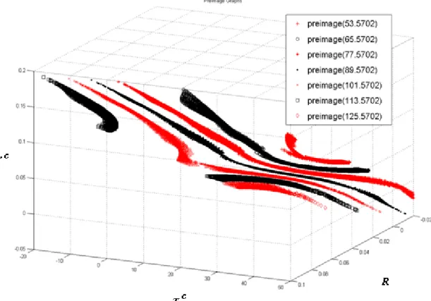
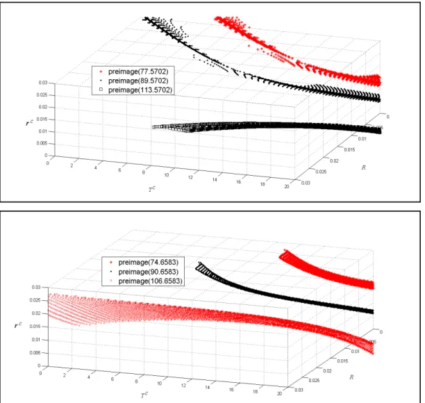
As shown in Fig. 2, the preimage f -1 is a complex 2-manifold. According to his beliefs, the
practitioner inspects relevant preimage-related properties. Take the following three beliefs as
the illustration. First, the practitioner knows that the type of a bond, premium or discount, can
be determined by comparing the market interest rate with the contract coupon rate. Specifically,
if the coupon rate is greater than the market interest rate, then the bond is priced as premium,
else as discount. This belief leads to an insight that the preimage of each reliable network
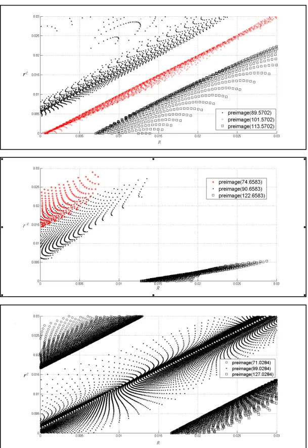
should be parallel to the plane with this property that rc = R. As shown in Fig. 3, the preimages
of all three networks show the tendency predicted by the insight. Thus, he gives this belief a
high credibility.
Second, the practitioner understands that one bond with a greater coupon rate than another
should be priced higher at a given interest rate. From preimage of each network in Fig. 3, he
observes that there is a positive relationship between coupon rate and interest rate. Namely, the
a high credibility and conjectures further that the high interest rate results in the low bond price.
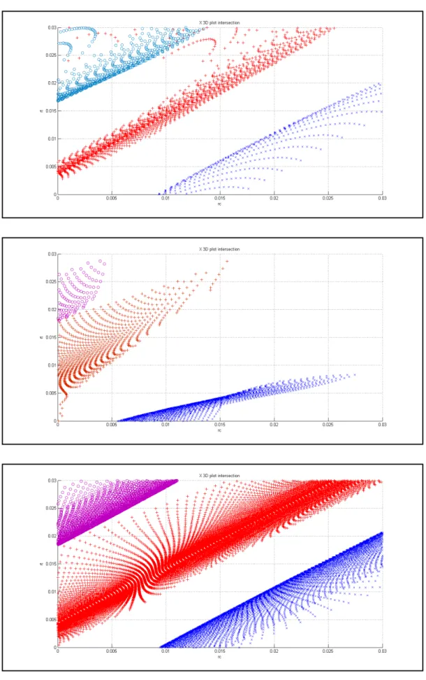
Third, from Fig. 4, the practitioner observes different curvatures for the premium bonds and
discount bonds in networks I and II, but not in Network III. Namely, in the rc and Tc
coordinates, the preimages for premium bonds appear to be concave and those for discount
bonds appear to convex for networks I and II. Thus, the practitioner gives low credibility to the
insight that, when the bond price is held constant, the rate of increase (respectively decrease) in
interest rate of a premium (respectively discount) bond increases as the maturity of the bound is
getting shorter.
IMPLICATIONSANDFUTUREWORK
The bond pricing experiment shows that the practitioner should have domain knowledge to set
up challenging propositions and collect the sample for network’s training as well as SLFN
knowledge to acquire reliable networks for feature discovery. And complex preimage-related
properties make the practitioner conduct belief justification process. For SLFN-p with p ≤ 3, the inspection of preimage-related properties could be conducted through the y-µ graph like Fig. 1 or the preimage graph in the input space like Fig. 2. For SLFN-p with p > 4, however, the
inspection of preimage-related properties relies on certain skills and experiences of nonlinear
Other possible future avenues of further enquiry may be the application of the proposed
preimage analysis to real world data and the externalization of belief into explicit knowledge
through SLFNs.
ACKNOWLEDGMENTS
This study is supported by the National Science Council of the R.O.C. under Grants NSC
92-2416-H-004-004, NSC 93-2416-H-004-015, and NSC 43028F.
REFERENCES
Andrews, R., Diederich, J., & Tickle, A. B. (1995). Survey and critique of techniques for
extracting rules from trained artificial neural networks. Knowledge-Based Systems, 8(6),
373-389.
Arslanov, M. Z., Ashigaliev, D. U., & Ismail, E. E. (2002). N-bit parity ordered neural
networks. Neurocomputing, 48, 1053-1056.
Baesens, B., Setiono, R., Mues, C., & Vanthienen, J. (2003). Using neural network rule
extraction and decision tables for credit-risk evaluation. Management Science, 49(3), 312-329.
Hohil, M. E., Liu, D. R., & Smith, S. H. (1999). Solving the N-bit parity problem using neural
networks. Neural Networks, 12(11), 1321-1323.
Hertz, J., Krogh, A., & Palmer, R. G. (1991). Introduction to the theory of neural computation.
Huang, G., & Babri, H. (1998). Upper bounds on the number of hidden neurons in feedforward
networks with arbitrary bounded nonlinear activation functions. IEEE Transactions on Neural
Networks, 9, 224-229.
Iyoda, E. M., Nobuhara, H., & Hirota, K. (2003). A solution for the N-bit parity problem using
a single translated multiplicative neuron. Neural Processing Letters, 18 (3), 213-218.
Lavretsky, E. (2000). On the exact solution of the Parity-N problem using ordered neural
networks. Neural Networks, 13(8), 643-649.
Liu, D. R., Hohil, M. E., & Smith, S. H. (2002). N-bit parity neural networks: new solutions
based on linear programming. Neurocomputing, 48, 477-488.
Munkres, J. (1975). Topology: a first course. New Jersey: Prentice-Hall Englewood Cliffs.
Murty, K. (1983). Linear Programming. New York, NY: John Wiley & Sons.
Nonaka, I., & Takeuchi, H. (1995). The knowledge-creating company. Oxford: Oxford
University Press.
Rabuñal, J., Dorado, J., Pazos, A., Pereira, J., & Rivero, D. (2004). A new approach to the
extraction of ANN rules and to their generalization capacity through GP. Neural Computation,
16, 1483-1523.
Rumelhart, D. E., & McClelland, J. L. (1986). Parallel distributed processing: explorations in
Rumelhart, D. E., Hinton, G. E., & Williams, R. J. (1986). Learning internal representation by
error propagation. In D. E. Rumelhart, and J. L. McClelland (Eds.), Parallel distributed
processing: explorations in the microstructure of cognition, vol. 1: foundation. Cambridge, MA:
MIT Press, 318-362.
Saito, K., & Nakano, R. (2002). Extracting regression rules from neural networks. Neural
Network, 15(10), 1297-1288.
Setiono, R., Leow, W. K., & Zurada, J. M. (2002). Extraction of rules from artificial neural
networks for nonlinear regression. IEEE Transactions on Neural Networks, 13(3), 564-577.
Setiono, R., & Liu, H. (1997). NeuroLinear: From neural networks to oblique decision rules.
Neurocomputing, 17(1), 1-24.
Setiono, R. (1997). On the solution of the parity problem by a single hidden layer feedforward
neural network. Neurocomputing, 16, 25-235.
Sgroi, D., & Zizzo, D. (2007). Neural Networks and bounded rationality. Physica A, 375,
717-725.
Taha, I. A., & Ghosh, J. (1999). Symbolic interpretation of artificial neural networks. IEEE
Transactions on Knowledge and Data Engineering, 11(3), 448-463.
Tickle, A. B., Andrews, R., Golea, M., & Diederich, J. (1998). The truth will come to light:
directions and challenges extracting the knowledge embedded within trained artificial neural
Tsaih, R., Hsu, Y., & Lai, C. (1998). Forecasting S&P 500 stock index futures with the hybrid
AI system. Decision Support Systems, 23(2), 161-174.
Tsaih, R. (1998). An explanation of reasoning neural networks. Mathematical and Computer
Modelling, 28, 37-44.
Urcid, G., Ritter, G. X., & Iancu, L. (2004). Single layer morphological Perceptron solution to
the N-bit parity problem. Lecture Notes in Computer Science, 3287, 171-178.
Zhou, R. R., Chen, S. F., & Chen, Z. Q. (2000). A statistics based approach for extracting
priority rules from trained neural networks. Proceedings of the IEEE-INNS-ENNS International
Table 4: the 18 hypothetical bonds with different combinations of term to maturity and
contractual interest rate.
Bond No. Term to maturity (T0) Contractual interest ratea (R) Bond No. Term to maturity (T0) Contractual interest rate (R) Bond No. Term to maturity (T0) Contractual interest rate (R) 1 2 0.0% 7 2 1.5% 13 2 3.0% 2 4 0.0% 8 4 1.5% 14 4 3.0% 3 7 0.0% 9 7 1.5% 15 7 3.0% 4 10 0.0% 10 10 1.5% 16 10 3.0% 5 15 0.0% 11 15 1.5% 17 15 3.0% 6 20 0.0% 12 20 1.5% 18 20 3.0% a
Tab le 5: final weights and biases of networks I, II and III, respectively. Weights and Biases Network O w0 j wHj0 O j w wHj1 H j w 2 H j w 3 I 100.4744 1 -0.1689 15.1206 -0.0347 -32.722 3 18.8396 2 -1.3535 -34.366 0 0.0544 -36.828 6 28.9551 3 -2.1615 5.6589 0.0988 43.3354 16.8267 4 1.1698 -21.999 9 -0.0643 -36.418 8 53.6646 II 93.6583 1 0.4510 -23.387 4 -0.0571 -33.464 8 71.8090 2 0.8413 36.9871 -0.0467 32.9078 -10.592 6 3 -1.1572 -10.462 1 0.0699 45.5792 43.2855 4 1.2874 -9.2684 -0.0458 17.5685 -87.314
7 III 104.8248 1 0.7832 -14.035 2 -0.0519 -27.129 9 49.3836 2 1.3108 -16.729 7 -0.0571 -27.374 8 14.5874 3 -1.5287 -30.181 9 0.0631 -37.1108 33.3026 4 -0.6010 13.1504 -0.0524 -34.904 2 36.9149
Figure 2: The preimage graphs of Network I. The numbers within the parentheses are values of
y.
Figure 3: Preimage graphs along the rc and R plane for networks I, II, III (from top to bottom),
Figure 4: Preimages graphs along the plane of rc vs. Tc for networks I, II, III (from top to
計畫成果自評:
本研究內容與原計畫相符程度高,達成預期之研究目的。不過,也發現其後續研究之有 趣以及困難處。本研究報告將加以修改後,投稿到學術期刊發表。
出席國際學術會議心得報告
計畫編號 NSC 97-2410-H-004-017 計畫名稱 利用 preimage 分析萃取規則之實作 出國人員姓名 服務機關及職稱 蔡瑞煌 國立政治大學資訊管理學系 教授會議時間地點 14-19 June 2009, Atlanta, Georgia
會議名稱 2009 International Joint Conference On Neural Networks (IJCNN2009)
發表論文題目 Knowledge-Internalization Process for Neural-Network Practitioners 一、參加會議經過
我於 16/06/2009 凌晨到達 Atlanta 後,於會場上聆聽多場 Plenary Talk 及多篇論文 之發表,亦於 16/06/2009 發表論文,於 17/06/2009 晚上離開 Atlanta 回國。附件是我 所發表之論文。
二、與會心得
Plenary Talk 邀請了不少的 Neural Networks 學界裡之知名學者,例如 John Hopfield, Bernard Widrow, John Taylor, Walter Freeman 等人,來演講,我受益不少。 我回國後,加以修改我所發表之論文,將投稿於期刊上。
Abstract—This study explores the knowledge-internalization process within which a neural-network practitioner embody the explicit knowledge obtained from extracting network’s preimage, the set of input values for a given output value, into his/her tacit knowledge. With a number of well-trained single-hidden layer feed-forward neural networks, the practitioner first extracts the (nonlinear) preimage of each trained network. The practitioner then internalizes the explicit outcomes and the insights obtained from the preimage extracting process into his/her tacit knowledge bases. We use the experiment of bond-pricing analysis to illustrate the knowledge-internalization process. This study adds to the literature by introducing the knowledge-internalization process. Moreover, in contrast to the data analyses in previous studies, this study uses mathematical analyses to identify networks’ preimages.
I. BLACK-BOXDILLEMAANDKNOWLEDGEACQUISITION
HEN practitioners apply Artificial Neural Networks (ANN) to resolving social science issues, there is a dynamic human process of justifying personal belief toward the “truth”. Reference [9] stated that ANNs can be trained (just as human children are taught), ANNs can learn primarily through example (as is often the case with humans), and ANNs can create general pattern-recognizing algorithms, learning general rules of optimal behavior. Since then, varieties of ANN have been developed and applied in many fields as modeling tools to see if the ANN does provide a model of human behavior and does approximate likely patterns of human behavior. At the beginning stage, a huge amount of experiments are conducted to see if the corresponding performances of the trained ANN are acceptable. Most experimental results are positive. For instance, [13] stated that ANNs “are consistent with observed laboratory play in two very important senses. Firstly, they select a rule for behavior which appears very similar to that used by laboratory subjects. Secondly, using this rule they perform optimally only approximately 60% of the time.” (p. 717) Later, the excitement shifts to applying ANN to resolving the challenging issue of domain. For instance, through extracting rules or features from a well-trained ANN, one tries to identify risk factors for newly issued securities, which have a prohibitively small number of observations. There are several concerns, however, when one has such application.
On the one hand, the practitioner has to cope with the
Manuscript received Feb 12, 2009. This work was supported in part by the National Science Council of the R.O.C. under Grants NSC 92-2416-H-004-004, NSC 93-2416-H-004-015, and NSC 43028F.
black box1
Rule: If the input sample is in some sub-region of the input
space, Then the predicted value is given by a corresponding linear regression equation. (1)
image of ANN to obtain a better understanding of relations between the input to ANN and its output. Reading or understanding the knowledge in ANN is difficult because the knowledge is distributed over the entire network and the relation between the input to ANN and its output is multivariate and nonlinear. Nevertheless, there is a huge amount of work that explore various “mechanisms, procedures, and algorithms designed to insert knowledge into ANNs (knowledge initialization), extract rules from trained ANNs (rule extraction), and utilize ANNs to refine existing rule bases (rule refinement).” [1, p. 373] Some, but not exhaustive, recent studies can refer to [1]-[2], [10]-[12], [14]-[15], [17]-[18]. These studies are contrived by the
engineering design with data analysis and approximation.
For instance, to identify the premise of a single rule stated in (1), most work use either training data or generated data, which the trained network itself yields. Due to the finite number of (training or generated) data instances, however, such a data analysis covers only some finite countable points in the (presumed) region of the rule premise, instead of the entire region. Reference [11] implemented a piecewise linear approximation on each hidden node to divide the input space into sub-regions in each of which, a corresponding linear equation that approximates the network’s output is defined as the consequent of the extracted rule to ensure the predicted value can be calculated from a comprehensible multivariate polynomial representation. Reference [3] solved the inversion problem through the back-propagation a union of polyhedra, which approximate (arbitrarily well) any reasonable set.
On the other hand, instead of a knowledge acquisition process, practitioners conduct a knowledge internalization process within which they embody the explicit outcomes and the insights obtained from the experiment into their tacit knowledge. Knowledge is normally tacit -- highly personal and hard to formalize. Subjective insights, intuitions and hunches are common heard from the discussions and sometimes difficult to replicate as the validation process depends on certain skills and experience. It is not trivial to conduct such knowledge internalization even when some explicit outcome is extracted from ANN. Furthermore, in most social science applications (e.g., financial market tests), the knowledge internalization process needs to cope with the
1 A black box refers to a system that produces “certain outputs from
certain inputs without explaining why or how.” [7, pg. 1483] The black box image for many years has gradually discouraged the study or application of the ANN.
Knowledge-Internalization Process for
Neural-Networks Practitioners
unlikely perfect learning due to the defect design of the architecture of ANN2
II. THE KNOWLEDGE INTERNALIZATION
and the garbled data. In literature, however, there are no discussions connecting to such knowledge internalization process.
This study explores such a knowledge internalization process. Specifically, the ANN used here is the real-valued single-hidden layer feed-forward neural networks (hereafter also referred to as SLFN) with one output node. Furthermore, the following assumption is set to help average out noises in estimates from individual SLFNs and serve as a stabilization measure to the knowledge internalization process: The practitioner should have a number of SLFNs, each of which is perceived well-trained by the practitioner, although does not necessarily provide a globally optimal learning result.
In order to not trap in the criticisms due to adopting the data analysis and approximation, mathematical analysis is adopted here to explicitly specify the (nonlinear) preimage of each SLFN’s mapping and thus the rule (2):
Rule: If (x ∈ the f -1(y’) region), then (y = y’), (2) where x is the vector of explanatory variables; y is the network’s response; f : X → Y is the function of the trained SLFN and y ≡ f(x); y’ is a constant; and the preimage f -1 is
the inverse function of f. The preimage f -1(y’) also represents the collection of inputs of the given output value y’.
The function representation f and preimage f -1 of the obtained SLFN are instances of explicit outcomes that can be “easily communicated and shared in the form of hard data, scientific formula, codified procedures, or universal principles” [6, p. 8]. When the practitioner conducts the experiment without domain expertise, the explicit outcomes and the insights obtained within the extracting process make some statement exclusively. But when there is certain prior belief, the practitioner focuses on the credibility of belief, the extent to which the belief can be generalized within the preimage-extracting process and the subsequent examination process. At the end of knowledge internalization process, the practitioner can have a posterior belief that has “high credibility” if the explicit outcomes and the insights obtained within the extracting process corroborate the belief; and “low credibility” if some corresponding result contradicts and weakens the belief. That is, when the explicit outcomes and the insights obtained within the extracting process are totally consistent with the practitioner’s prior belief, he/she may accord his/her belief a high credibility. Conversely, an inconsistent result triggers the following examinations of SLFNs and belief instead of an immediate rating:
(i) Investigating whether there exist factors or noises leading to a defect design of the SLFN such that all well-trained SLFNs are not suitable for the purpose of rating the credibility of belief.
(ii) Examining whether some of the obtained SLFNs are optimal to the extent that they are suitable for the
purpose of rating the credibility of belief.
(iii) Consolidating the explicit outcomes the obtained insights amongst all reliable SLFNs.
(iv) Contrasting the belief with the consolidated outcome of reliable SLFNs.
Only when the practitioner feels certain that he/she can eliminate the first possibility, should he/she rate the credibility of belief. Furthermore, the practitioner would conservatively follow the explicit outcomes and the obtained insights.
Section III uses the experiment of bond-pricing analysis, which in literature is a nonlinear regression problem with continuous variables, to illustrate the knowledge internalization process. At the end, conclusion and future work are offered.
III. THEBONDPRICINGEXPERIMENT
In order to simulate the set of data that may be observed by a representative practitioner, who know about the bond-pricing mechanism well (but less than perfectly), garbled training samples of bond price yt = pt + εt are generated and used. pt
is the theoretic value of the bond at time t and is derived from (3), which serves as an example of complete domain knowledge with respect to the bond pricing model, and εt is
a white error term provided by a normal random number generator of N(0, (0.2)2). Namely, yt is perturbed by a white
noise. pt ≡
∑
= + − 0 1(1 ) T k t k t r C + t T t r F − + )0 1 ( (3)According to (3), pt is determined by (i) rt, the market
rate of interest at time t; (ii) F, the face value of the bond, which generally equals 100; (iii) T0, the term to maturity at
time t = 0; and (iv) C, the periodic coupon payment, which equals F×rc. As depicted in Table 1, we use 18 hypothetical
combinations of term to maturity and contractual interest rate and generate a set of price data with t = 1/80, 2/80, …, 80/80 through (3). The rate rt is derived from a normal
random number generator of N(2%, (0.1%)2
). Accordingly, we have 1,440 training samples with input variables Tt, rc
and rt, and the desired output variable yt, where Tt ≡ (T0 - t)
is the term to maturity at time t.
To examine the generalization of trained networks, we also generate 1,440 test samples by the similar means, except that T0, t, rc and rt are randomly and independently
generated from {1, 2, …, 20} with a probability of 1/20 for each, {1/80, 2/80, …, 80/80} with a probability of 1/80 for each, [0.0%, 3.0%] with a probability density function f(rc) =
1/0.03 and N(2%, (0.1%)2), respectively. This setting results
in varying instances among the test samples.
We, as the representative practitioner, adopt the Back Propagation learning algorithm [8] to train 1,000 SLFNs, each of which has 4 hidden nodes and random initial weights and biases. Among the 1,000 SLFNs, we pick the three with the smallest mean square error (hereafter, MSE) for the test
respectively. The corresponding MSEs for the training samples are 0.414, 0.404 and 0.451, respectively; and the corresponding MSEs for the test samples are 0.429, 0.432 and 0.445, respectively. The average absolute deviation is approximately 0.6, which deviates from the specified error term standard deviation of 0.2. The pricing error is unrelated to theoretic prices pt. but related to observed prices yt.
By definition, for each SLFN, the hth activation value ah
equals tanh(bhH+ 3 1 = ∑ i H hi
w xi), h = 1, ..., 4; the output y equals
bo + 4 1 = ∑ h o h
w ah; and the function f equals bo +
4 1 = ∑ h o h w tanh( H h b + 3 1 = ∑ i H hi
w xi). Hereafter, let (⋅)T be the transpose of (⋅) for (⋅) to
be a vector or a matrix. Furthermore, o
h
w ≡ the weight of the hth activation value for the output,
where the superscript o throughout the paper indicates quantities related to the output layer;
bo ≡ the bias of the output node;
H hi
w ≡ the weight of the ith input for the hth hidden node, where the superscript H throughout the paper indicates quantities related to the hidden layer;
H h⋅ w ≡ ( H h w1, H h w2, H h w3) T
, the 3x1vector of weights between the hth hidden node and the input layer;
WH ≡ ( H ⋅ 1 w , H ⋅ 2 w , H ⋅ 3 w , H ⋅ 4
w )T, the 4x3 matrix of weights between
the hidden nodes and the input layer; and H
h
b ≡ the bias of the hth hidden node.
For ease of reference in later discussions, we also call R3 the
input space and (-1, 1)4 the activation space. For each SLFN, f -1(y) = Φtanh-1。Φo-1(y), with
Φo-1(y) ≡ {a ∈ (-1, 1)4| 4 1 = ∑ h o h w ah = y - bo}, (4) Φtanh-1(a) ≡ 4 1 1 -T } -) ( = | { = ⋅ ℜ ∈ h H h h H h tanh a b w x x 3 , (5)
where Ω is a subset of ℜ and tanh-1(x) ≡
( )
-xx1 1 ln 5 . 0 + . Formally, the followings are defined for every SLFN:
(i) A value y ∈ ℜ is void if y ∉ f({ℜ3}), i.e., for all x ∈ ℜ3,
f(x) ≠ y. Otherwise, y is non-void.
(ii) A point a ∈ (-1, 1)4 is void if a ∉ Φ
tanh({ℜ
3
}), i.e., for all x ∈ ℜ3, Φ
tanh(x) ≠ a. Otherwise, a is non-void. The
set of all non-void a’s in the activation space is named as the non-void set.
(iii) The image of an input x ∈ ℜ3 is y ≡ f(x) for y ∈ Ω.
(iv) The preimage of a non-void output value y is the set f -1 (y) ≡ {x ∈ ℜ3
| f(x) = y}. The preimage of a void value y is the empty set.
(v) The internal-preimage of a non-void output value y is the set {a ∈ (-1, 1)4| Φ
o(a) = y} on the activation space.
Given the weights and biases of each SLFN, the preimage-extracting phase conducts the following steps, where rank(D) is the rank of the matrix D and [D1 D2] be
the augmented matrix of two matrices D1 and D2 (with the
same number of rows):
Step 1: Derive the expression of Φo-1(y);
Step 2: Derive the expression of the non-void set that is defined as {a| rank(WHω(a)) = rank(WH)};
Step 3: Derive the expression of A(y) that is defined as {a|
a∈ Φo-1(y) AND rank(WHω(a)) = rank(WH)}; and
Step 4: Derive the expression of f -1(y) that is defined as {x|
WHx = ω(a) with all a ∈ A(y)}.
Take Network I to illustrate the explicit outcomes and the insights obtained within the extracting process. Φo-1(y) =
{a| 15.1206a1 - 34.366a2 + 5.6589a3 - 21.9999a4 = y -
100.4744}. Φo
-1
(y) is in the form of linear equation. Thus, for each non-void value y, Φo-1(y) is a hyperplane in (-1, 1)4.
As y changes, Φo-1(y) forms parallel hyperplanes in (-1, 1)4;
for any y changes of the same magnitude, the corresponding hyperplanes are spaced by the same distance. The activation space is entirely covered by these parallel Φo-1(y)
hyperplanes, orderly in terms of the values of non-void y. Furthermore, the center of these parallel hyperplanes is the Φo-1(100.4744) hyperplane. These parallel hyperplanes form
a (linear) scalar field: For each point a of the activation space, there is only one output value y whose Φo-1(y)
hyperplane passes point a; all points on the same Φo-1(y)
hyperplane are associated with the same y value. Note that the function xT H
h⋅
w = tanh-1(ah)
-H h
b within the
hth component in the right-hand side of (5) is a separable function from the one within the other components. Given an activation value ah, {x ∈ ℜ3| xT H h⋅ w = tanh-1(ah) -H h b } defines a hyperplane in the input space, since all H
h⋅ w and H
h
b are given constants. For the hth hidden node, the hyperplanes associated with various ah values are parallel
and form a (linear) scalar activation field in the input space [16]: For each point x of the input space, there is only one activation value ah whose corresponding hyperplane passes
point x; all points on this hyperplane are associated with the same ah value. Furthermore, each hidden node gives rise to
an activation field in the input space, and four hidden nodes set up four independent activation fields in the input space.
4 1 1 -T } -) ( = | { = ⋅ h H h h H h tanh a b w x x in (5) can be denoted by
{x|WHx = ω(a)}, where ω(a) ≡ (ω1(a1), ω2(a2), ω3(a3),
ω4(a4))T and ωh(ah) ≡ tanh-1(ah)
-H h
b for all 1 ≤ h ≤ 4. Given
the activation values of a, ω(a) is simply a vector of known component values and the representation
WHx = ω(a) (6)
is a system of four simultaneous linear equations with three unknowns. Furthermore, WHx = ω(a) is a set of inconsistent
simultaneous equations if rank(WHω(a)) = rank(WH) + 1 [5, p. 108], and thus the corresponding point a is void. The discussion establishes Lemma 1 below.
Lemma 1. An activation value a is void if rank(WHω(a)) = rank(WH) + 1; otherwise, a is non-void.