Maneuvering target tracking with colored noise

Maneuvering Target Tracking

with Colored Noise

WEN·RONGWU DAH.CHUNG CHANG

National Chiao Thng University Thiwan

It is known thai colored noise may degrade the performance of a tracking algorithm. A common remedy is to model colored noise as an autoregressive (AR) process and apply the measurement difference method. One problem with the approach is that the AR parameters are usually unknOWIL In this work, we propose a new method to adaptively estimate the AR parameters. It is shown that this method is simple and practically feadble. We incorporate our method into the interacting multiple model (IMM) tracking algorithm and _how that the performance is almost as good as that. in the known parameters case.

Manuscript received June 10, 1994; revised May 10 and August 24, 1995.

IEEE Log No. T·AESJ32/4/08000.

Authors' address: Department of Communication Engineering, National Chiao Thng University, Hsinchu, Taiwan, R.O.c.

0018·9251/96/$5.00 © 1996 IEEE

I. INTRODUCTION

A white noise observation model is widely

used in tracking problem formulation. In practice,

the measurement noise may not be white. This

phenomenon is due to the scintillation of the target.

Typically, the bandwidth of measurement noise

is on the order of several hertz [3, 12]. When the

measurement frequency is much lower than the

noise bandwidth, the successive samples of the

noise are approximately uncorrelated, and it can be

seen as white. However, in many radar systems, the

measurement frequency is high enough so that the

correlation cannot be ignored without degrading the

tracking performance.

The conventional method that alleviates the effect

of colored noise is the state augmentation approach

[1]. But this may cause the covariance matrix to be

ill·conditioned. Bryson [2] proposed the measurement

difference approach to prevent the problem. Rogers

[3] modeled the colored noise as a lst·order AR

process and applied the measurement difference

approach to the a-f3 filter. Guu and Wei

[4] extended

Rogers' method in [3] to maneuvcring target tracking

problem using the interacting multiple model (IMM)

metho

d

. Besides

d

escrete·

t

ime approaches, some

researchers also investigated the continuous-time

Kalman tracker under the colored noise environment.

Rogers [6] derived closed· form solutions for the

tracker with exponentially correlated velocity (ECV)

and exponentially correlated acceleration (ECA).

Arcasoy

[7] used the spectral factorization method

to

develop cx

pr

c

s

sio

ns

of

the Kalman gains for the

ECV and ECA tracking problems. In aforementioned

approaches, they all assumed that the a

u

tor

e

g

res

si

v

e

(AR)

coefficients are known. However, this may

not be possible in the real applications. GUll and

Wei

[5] then further developed a method to estimate

the AR parameters. Unfortunately, this method is

computationally intensive and only applicable to the

Makovian acceleration model.

It cannot be used in

some advanced tracking algorithms such as IMM.

We propose a new method to estimate the AR

parameters. We first remove the state variables from

measurements by passing them into a moving average

(MA) filter and this results in an autoregressive

moving average (ARMA) signal. it is found that

the z-transform of the signal has two zeros on the

unit circle. In order to obtain the AR coefficient

from the ARMA signal, we further introduce an

AR filter to cancel the zeros. The AR parameters

are then calculated from the statistics of the output

signal. However, when the target is maneuvering, the

estimates will be biased. From theoretical analysis,

we derive a closed·form solution to remove the bias.

OUf method

can

be

implemented adaptively and is

suitablc for on·line processing. Simulations show that

our method can estimate the parameters precisely. The

proposed algorithm and the measurement difference method are used in the IMM algorithm and significant improvement is obtained.

II. DECORRElATION PROCESS

In this section, we describe the decorrelation process in [3]. For simplicity, we assume that states of target motion are defined in the spherical coordinate sueh that the state equations can be decoupled into three independent channels. Then, the tracking filter can work independently on each channel [9]. The state equations in a particular channel can be described as follows

Xk+1 = ¢Xk

+ GWk

Yk =HXk +Vk

(1)

(2)

where

Xk

is state vector, ¢ is state transition matrix, Yk is the measurement, Wk and

Vk

are the state and the

measurement noise, respectively. If the measurement frequency is high, the correlation of

Vk

cannot be ignored. Rogers

[3J

modeled the continuous colored noise as a first-order AR process, which can be described as

(/(t) = -).,u(t

)

+

fJ(t).

(3) Sampling

u(t

)

with a period

T,

we obtain a difference equation which is

where 0:

=

e->'T

and

17k

is zero-mean white

Gaussian noise with variance

O'�.

To decorrelate the measurement noise, a new measurement

Yk,

called "artificial measurement," is generated

where _

6-Yk =6-Yk - O:6-Yk-l

= H(Xk

- O'Xk-l)

+

(JJk

- O:Vk-l)

= HXk +fik

H =

H(1-

o:¢-l)

fik

=

O'r1Gwk_l

+ fJk·

In practical applications, the first term of right-hand side in

(7)

is usually small and can be neglected. So, we have

T hus, fik can be treated as white. Now, the new measurement equation (5) and the original state equation (1) can be used in the Kalman filtering. III. ESTIMATION OF AR PARAMETERS

In the previous section, we sec that if the AR parameters (0: and

0',/)

are known, the colored noise

(4)

(5)

(6)

(7)

can be decorrelated. However, it is difficult to know thc parameters in the real application. Here, we propose a method that can effectively estimate the parameters. For the ease of description, we assume that thc measurement is the position of the target. Let

X

k "" [Xb Vbakf

where

Xb Vk,

and

ak

are position, velocity, and acceleration of the target, respectively, we then have the measurement equation

(9) Since measurements contain state variable

Xk,

the direct estimation of AR parameters is difficult. It will be very helpful if we can remove state variable Xk. From the Newton's law, we have

(10)

We now use the following operation to obtain a new . signal

lh

that does not involve Xk

Uk

= Yk -

2Yk-l +

Yk-2

=

(Yk -

Yk-l) -

(Yk-l - Yk-2)

= (Uk - 2JJk_l + Vk_2) + (Xk - Xk-l)

- (Xk-l - Xk_2)

= (Uk - 2Uk_1 + Uk-2) + !Cak-l + ak_2)T2.

(11) A close look reveals that the operation is essentially a MA filtering and it can completely null a linear function

(ak = 0).

When the measurement frequency is high, the measurement (without noise) is approximately linear in a short period of time (in our case, two

T8).

T hus, this simple filtering operation enables us to extract the measurement noise with little distortion. To investigate the effect of the filtering, we go to the transform domain. Taking the

Z

-transform of (11), we have

where

U(Z)

= (1- 2z-1 + z-2)v(Z)

+

m(z)

=

(1- [1)2u(z)

+ m(z)

(12) (13) Note that

JJk

is an AR process. From

(4),

we find its transfer function is

1

JJ(z) =

1--

o:z-ll)(Z).

Thus, we can represent

u(z)

as

(1-

Z-1

)

2

u(z) =

1-ar

1 7/(Z)

+ m(z).

(14)

(15)

When the target is nonmaneuvering, the acceleration is zero and

m(z)

is zero. From (15), we know

Uk

is an ARMA process. Since there are two zeros on the unit circle, it is difficult to use the general system

identification methods to estimate the AR coefficients. To overcome this problem, we further introduce a filter to cancel the zeros. Consider the filter described by its transfer function as follows

1

F(z) -

- (1- prl)2

-:-:---�

(16)

where

0

s:

p

s: 1. Passing

u(z)

through

F(z),

we obtain the output (denoted as

u(z»

(1- z-I)2

_

u(z) = (1- prl)2 u(z)

(17)

1 (1-

Z-Ip

m(z)

1-

o:rl

(1-

pZ-l)21J(Z) + (1- pr1)2'

(18) For

nonmaneuvering cases, the second term of

the right-hand side

in

(18) is

zero. If we let

p

=

1,

zeros are completely canceled. From (18), we sec that Uk is just the colored noise vb i.e.,

(19)

Denote the autocorrelation function of Uk as

reo).

The 0: can then be estimated by

, r(l)

0: ""

r(O)'

(20)

Here, we use an adaptive method to estimate the

autocorrelation function. By

the fading memory technique [151, we have

i'k(O)

=

f:Jh-l(O) + (1- f:J)u�

(21) (22) where 0 <

(3

< 1 is the forgetting factor. If (3 is

large, the convergence of PO is slow and it cannot response to the change of 0: quickly. The advantage

of using large f3 is the small estimation variance. On the

contrary, small f3

will let

PO

converge fast and response quickly. However, the estimation variance

is

large.

When the target is maneuvering,

m(z)

is not negligible. In this case, we cannot choose

p

as one,

otherwise the low frequency components of

m(z)

will be greatly amplified. It is easy to see this from the Fourier transform of

F(z)

IF(eiW)1 = \1-:e-

jw

r

1

(1 + p2) - 2pcosw .

(

2

3

)

The magnitude in (23) will become huge if

p = 1

and

w is small (infinite for

w = 0).

This will breakdown

the whole algorithm. Therefore,

p

cannot be one. From experience, we find that if

p i

s

0.9

or less, the amplification effect is small compared with the first term

of

(18). With suitable choice of

p,

we can then

Fig. 1. Algorithm of estimating AR coefficient of colored noise.

ig

n

or

e

m(z). T

h

u

s,

1

(1_Z-1)2

u(z)::::! 1- o:rl (1- pz-l)21J(Z).

₍₂₄₎

However, the nonunity

p

raises another problem. From

(24),

it is clear that Uk is

no

longer

equal

to

Vk and

r(l)

0:

t=

reO)"

(25)

The estimate

of

(20)

is then biased. To correct the bias, we explore the relation of 0: and

r(l)/r(O).

Equation

(24)

can be rewritten as

[1- (2p + O:)Z-1 +

(2ap

+

p2)z-2 - o:p2z-3Ju(z)

(26)

Thus,

u(z)

is an ARMA process. Using the Yule-Walker equations [15], we can s

ol

ve for its coefficients in terms

of

its autocorrelation function. Let

b r(1)

0: =

reO)

(27)

6

=

(p

+

Ii

(28)

6 =

(_2p2 -

lOp - 4) + (-6p

-

2)o:b

(29)

(30)

�o = (

2p

2 +

2p

- 4) + (-2p - 6)o:h.

₍₃₁₎

Then, 0: and

(J�

can

be

found as follows. We leave

derivation details in Appendix A

and

-(6

+

6)- )(6 + 6)2_46(6 + 6 +

�1)

Q =

26

[-2/0:2 + (1- p4)a +

2p]r(0)

(32)

+[(p2 + p4)0:2

+

(2p3

_

2p)0: _

(p2

+

l)]r(l)

(1 + p2)0:

+

(2p

-

4)

(33)

Substituting o:b with its estimate

<'ii,

we can obtain

<'ik

and

a-�,k'

The block diagram of our proposed algorithm is shown in Fig. 1.

In this paragraph, we estimate the computational requirement of our algorithm. Since the computational complexity of a multiplication/division is much higher than that of an addition/subtraction, we then ignore the operations of addition and subtraction in our complexity estimate. From Fig. 1, we know that

there are three stages in our algorithm. First, we use (17) to extract colored noise. Second, we use (21), (22), and (27) to calculate o:b. Finally, we use

(28)-(33) to estimate 0: and

O"�.

Totally, we need

26 multiplications, two divisions, and one square root operation for one cycle. It is shown that

[13]

a Kalman filter with scalar observations requires 4

n

3 +

2.5n2

+

3.5n

+

3

multiplications where

n

is the state dimension. The mixing operations in an IMM algorithm require

2:::1 (2nr

+ 2

n

i + 4) multiplications

and

m

exponential operations where

m

is the number of models and n; is the dimension of the ith modeL

For example, if we use two models in the IMM algorithm; one is 2-dimensional and the other one is 3-dimensional, a complete IMM algorithm will require 240 multiplications and two exponential operations. The computational complcxitics of the square root, division, and exponential operations are much higher than multiplications. It is difficult to have a precise evaluation. Roughly, we can say that the computational complexity of our algorithm is approximately one-tenth of the IMM algorithm.

Though Guu and Wei

[5]

also used the

measurement difference method to decorrelate colored noise, their AR identification algorithm is different from ours. They assumed that the acceleration of the target, ak> is a first-order Markov process (AR process), i.e.,

where

(k

is a white Gaussian process,

0";

== E{fn is unknown, and T is assumed to be known. They

define the innovation of the artificial measurement

(

3

4)

Yk

as

'ljJk

==

Yk

�

h; h

is the prediction of

Yk'

Using the correlation functions of

1/Jk, f!j

==

E{1J;k1);k-j},

j

== 0,1, . .. , Guu and Wei derived the following relationship

j

== 0,1, ...

(35)

where

fj

is a scalar and

gjO

is a nonlinear function of 0:. To solve

(35),

a

nonlinear algorithm was used to

minimize a least-squares criterion

where

ih

is an estimate of (! j based on

the

innovation sequence. T he problem of this approach is that many matrix and

vector operations

are required

to obtain fj

and

gj{-);

it is

computationally

intensive. In addition, the nonlinear minimization algorithm may converge to a local minimum.

IV. SIMULATION RESULTS

In this section, we carry out some simulations to demonstrate the effect of the proposed algorithm. For simplicity, we only consider a one-dimensional

range tracker herein. The IMM is applied as the tracking algorithm, which is implemented by using a second-o�der model for the nonmaneuvering mode and two third�order models for the maneuvering mode, one is with process noise and the other is without process noise. They are described in the following equations.

1)

Nonmaneuvering mode:

2)

Maneuvering mode:

[1, [�I In [1+

(38)

where

Wk

and

wk'

are white noise�. The measurement equation is

(39)

The Markovian transition probability matrix in IMM is

chosen as

[

0.99 0.01 0.00

]

[Pij]

== 0.33 0.34 0.33 . 0.00 0.01 0.99

In this simulation, the sampling period is taken as 0.05 s. The total tracking interval is 60 s. In

(40)

other words, there are 1200 measurement samples. The maneuvering occurs on 20th s to 40th s with constant acceleration 40 m/s2 (about 4g). The state noise variances are

E[WkWk]

== 10-3 (m/s2)2 for the nonmaneuvering mode and

E[wk'wk']

== a (m/s2)2, 8002 (m/s2)2 for the maneuvering mode. We assume that the standard deviation of measurement noise is

O"y == 100 m. Two AS are used in the simulations. One is

4

s-l and the other is 10 S-l. The corresponding 0: values are 0.8187 and 0.6067, respectively. The

simulation setup is the same as that in r4]. 100 Monte Carlo runs are carried out and the average results are shown under the root mean square error (RMSE) criterion

RMSE(k) =

! texk

-

ri)2

;=1

k

=

1,2, ... ,1200;

m ==

100 (41) where

xie

denotes state estimate of the ith Monte Carlo run for the kth sample.

We first cxamine the behaviors of the roots in

(32).

Fig. 2 shows the plot of 0: versus o:b for different

p values. Note that not all o:b is legitimate. The

value inside the square root in (32) must be greater than or equal to zero. From Fig. 2, we sec that if p approximates to one, the corresponding curve will be 1314 IEEE TRANSACTIONS ON AEROSPACE AND ELEC1RONIC SYSTEMS VOL.

32,

NO.4 OCTOBER

1996

0.8 0.6 0.4 0.2 -0.2 -0.4 (1), P = 0 (2), p -0.1 m 'P= 0.2 (,I), p = 0,3 (;)'p=0.4 (6) 'P = 0.5 (7): p = 0,6 (8) :p=O.1 (9) 'P = 0.8 (10),p=0.9 -0.4 -0.2 a 0.2 0.4 0.6 0.6

biased correlation coeff.

Fig, 2. Behavior of correct root for different

p,

completely linear with unit slope. This implies that the estimator in (20) yields unbiased estimates. If

p

::j: 1, the estimate is biased. Also note that for smaller

p

the slope of the curve is larger. This indicates that the

O,5�---0.45 o 200 � P =0.97 ....-.... P =0.90 ---p =0.60 400

resolution for Cib is p oorer. This will adversely affect the Ci estimate. All the curves in Fig. 2 are above the line 0: = o:b and pass through (-1, -1). In addition, their slopes are increasing. Thus, we can say that the larger the Ci is, the more bias Ci will have. For 0: = -1,

there is almost no bias.

To further study the effect of

p,

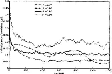
we plot the estimates for the whole tracking interval. Here, we assume that Ci = 0.8187 for whole interval. Figs. 3

and 4 show the results of

O:k

and (J ",k estimates for

different

p

values. The (3 is taken as 0.99. Generally, we find that larger

p

will have better results. However,

too large

p

will amplify the

mk

term in (18) when target is maneuvering. This results in poorer results. For

p

= 0.9, we see that the estimates are almost not

affected by maneuvering. In the case, the estimate error of Ci and (J" is around 0.075 and 4, which is

quite small

«(J'I

= 57.4). We also simulated another case that 0: = 0.6067. The results are similar to those

obtained previously and is therefore not shown. One

600

samples BOO 1000 1200

Fig. 3. Relation of

a

estimation error and

p (a

=

0.8187, (3

=

0.99).

30 mrr---r---�---._---,_---,_---� 25 5 o 200 -&-e- P =0.97 ... P =0,90 -- P=0.60 _{'-'-' p=O.20} 400 600 samples BOO 1000

Fig. 4. Relation of 0',., estimation error and

p (<Til

=

100, (3

=

0,99).

WU &

CHANG: MANEUVERING TARGET TRACKING WITH COLORED NOISE

1200

-0.8

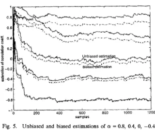
In Fig.

5,

we show the simulation result (single realization) for the estimation of O! with and without

bias. Five O! values are used. They are

0.8, 0.4, 0, -0.4,

and

-0.8.

We set p =

0.9

and f5 =

0.995.

It is clear that for smaller 0:, the bias is smaller. This agrees with our

induction from Fig.

2.

As aforementioned,

D:k

is adaptively estimated and the convergence rate depends on the f5 value. Smaller f3 has better tracking property but the estimation error is

larger.

To investigate the tracking property,

-1

0�----720�0----�40�O---6=O�O----�8=O�O----�100�O----�12'O

O samples

we now let O!k ""

0.8187

for nonmaneuvering period

and

O:k

""

0.6067

for maneuvering period. Note that

O!k

experiences abrupt changes during the tracking period. Figs. 6 and 7 show the performance of estimates of

O:k

and (J",k for different f3 values. Here, we set

p = 0.9.

In this experiment, we initiate the tracker

40

s before the formal tracking period. The purpose is to investigate the steady state behavior of our algorithm. From the figures, we verify the statement made Fig. 5. Unbiased and biased estimations of Q = 0.8, 0.4, 0, -0.4,

and -0.8

(p

= 0.9).

thing different is that for p =

0.97,

the amplification of

mk

is more serious than that in 0: =

0.8187.

However,

for p =

0.9,

the estimate is almost not affected.

1316 O.5'---�----�----�----r-___ _ --, ___ --, 0.45 0.4 � 80.35 � o

i

0.3 8 '00.25

g

� 0.2 o � .1'00.15 i � G�0.995 -- fJ�O.990 --f3 �O.985 - - ,3 =0.980 °O�---�2�OO�---4�O�O---6=O�O---�80�0�--� 100�O-­ samples

Fig. 6. Relation of _0' estimation error and

p (p

= 0.9).

1200 30,---�----.---_r---�---r_---� --e--e-- B =0.995 --f3�.990 25 -- a �O.985 - - ,9 -0.980

°O;----�2�OO�----4�0�O�--�60�0�---�8�O�O---,�O�070---�,200

_samples Fig. 7. Relation of _Ir� estimation error and

p (p

= 0.9).

o

-e-iT-Undecorrelated (cotored noise)

- - Exactly decorrelated (known parameters)

--Our _approac;h (unknown parameters)

100 200 300 400 500 600 700 BOO 900 1000 1100

samples

Fig. 8. Performance of position tracking in colored noise

(p

=

0.9, f3

=

0.99).

2i .§. g '" go :g � ... . .,

�

120

-G--G-Und�c::ol'mlatAd (Colored noise)

- - Exactly decorrelated (known parametera.)

100 --Our approach {unknown para.meters) BO 60 40 20 oL---₁₀₀ �--₂₀₀ �--₃₀₀ �--₄₀₀ �--₅₀₀ �--�--�_{GOO 7} --�--�--���--� 00 900 000 1000 1100 samples

Fig.

9.

Performance of velocity tracking in colored noise (p =

0.9, (l

=

0.99).

before. For f3 ==

0.99, we

find that it provides a

good compromise between conv

e

rgence rate and estimation error.

From

the

above result,

we know that p sho

u

ld be used as large as possible. The ma

i

n

factor limit

we show the tracking

performances for cases without deeorrelat

i

on, w

i

th

e

xact decorrela

t

ion

(

give

n the AR

parameters), and with the p

ro

posed decorrelation scheme. We

assume ak

=

0.8187

for target nonmaneuvcring period and

ak

=

0.6067

for maneuvering period. The rest of the paramet

e

r

s

are chosen as p =

0.9

and

f3

=

0.99.

This choice pis

mk. Fr

om (13), we f

in

d mk

i

s determined by

tar

g

e

t

acce

l

eration ak and sampling period T. If T is sma

l

ler,

l

ar

g

e p can be

used. Thus, we

can conclude that the higher the measurement frequency is, the better o

u

r al

g

orith

m will

work. f3 determines the tracking property and should be chosen ac

c

ording to ho

w

fast a will change. For

slow

changing a,

f3

can be

large. It see

m

s that negative a

is

ea

s

ier to

work

with

(

s

m

a

l

l bias). This can be explained by thc fact that

can make the estimation of a and (J' n insensitive to

maneuvering and abrupt changes of

parameters. From

these figures, we can dearly see that the performance of the decorrelated scheme is considerably better than that of

u

ndecorrelat

e

d one, special

l

y

in

the velocity the position

m

easure

m

ent is a low

-

pass signal while

the colored noise is a high-pass signal (for

n

egative a). Thus, it is easier to fil

te

r

o ut the

noise.

Finally, our approach is applied

to the m

ane

u

vering target tracking with colored noise. In Figs

. &-10,

and

acceleration estimates. The

performanc

e

of the proposed a

l

gorith

m

is almost as

g

ood

as that in

th

e

known paramcters casco Thc structure of the proposed algori

t

h

m

is s

im

ple and practically feasible. Also,

it

can adaptively track the variation of the AR para

m

eters.

This makes our algorithm is suitable for real-time applications.

-e-e--UndecorreJated (colored noise)

- - Exactly dscorrglated (known parameters)

50 -- Our approach (unknown parameters)

100 200 300 400 500 600 700 800 900 1000 1100

samples

Fig.

10.

Performance of acceleration tracking in colored noise (p =

0.9, f3

=

0.99).

V. CONCLUSION

We have proposed a new algorithm to identify the

parameters

of colored

noise, which can be applied

to maneuvering target tracking. Our algorithm is

different from that of Guu and Wei [5]. We do not

need the assumption of Markovian acceleration for

the maneuvering target. Thus, the IMM algorithm

can be used to achieve better tracking performance.

From simulations, we

find that our algorithm identifies

the parameters properly such that the tracking

performance is

almost

as good as that in the known

parameters case. The

simple structure

of the algorithm

makes it easy

to

be implemented.

In

(2), we assume

that the only noise component is colored noise

1Jk

which is modeled

as a first-order

AR

process.

If other

kind of noise such as white noise also exists, the mixed

noise will not

be

an AR process any more. It can be

shown that an AR

process

plus a white

process

is

an ARMA process [14].

In this case,

our algorithm

becomes a suboptimal

approach.

APPENDIX A

The Yule-

Walkcr equations

of (26) are

reO) - alr(l) - a2r(2)

- a3r(3)

=

(ai

- 4al

+

a2

+

6)0';

(42)

-

a

1r(0)

+

(1- a2)r(1)

- a3r(2)

=

(a1

-

4)()'�

(43)

-a,r(O)

-

(a,

+

a3)r(1)

+

r(2)

=

0';

-a3r(0) -

a2r(1)

- alr(2)

+

r(3)

=

0

where

al

=

2p + 0:

a2

=

-(2po: + p2)

a3

==

p20:.

(44)

(45)

(46)

(47)

(48)

Substituting r(2) and r(3) in (42) and (43)

by

using

(44)

and

(45), we have

(a� + a1a2a3 + a� - l)r(O)

+ (al +

alal

+

2alG3

+

ara3

+

ala

�

)r(l)

+

(ai

- 4al + 2a2 + ala3

+

6)O'�

=

0

(49)

and

(al + Q2a3)r(O) + (a2 + a1a3 + a� -1)'(1)

+

(al

+

a3 - 4)O'�

=

O.

From

(46)-(50), we have

(50)

[_2p30:

3 +

(4p2 - 4l)02 + (4p3 - 2p5)0:

+

l-l]r(O)

+

[(p2

+

p4)0:3

+

(2p5 _ 2p)0:2

and

+ (2p4 -5p2 + 1)0

+

(2p - 2p3)],(1)

+

[(1

+ p

2

)

Q

2

+

(2p3 - 4)0:

+ (2pl_ 8p + 6)]O'�

=

0

[_2p30:2

+

(1-p4)0: + 2p]r(0)

(51)

+ [(p2

+

l)a2 + (2p3

_

2p)a

_

(p2

+

1)],(1)

+

[(1 + l)a + (2p - 4)JO'�

=

O.

(52)

From (52), we yield

[_2p3o;2

+

(1- p4)0: + 2p]r(0)

0'2 =

_

+[(p2 + l)a2 + (2p3 - 2p)0: - (p2

+

1)]r(1)

1/

(1

+

p2)0:

₊

(2p - 4)

Replacing O'� in (51) by (53) and simplifying the

equation, we have

(53)

(54)

where

6

=

(p + 1) 3

(55)

6

=

(_2p2 - 10p

-

4)

+ (-6p

-

2)oJ}

(56)

el

=

(_p3 - 3p2 + 5p + 7) + (8p + 8)ab

(57)

eo

=

(2p2 + 2p

-

4)

+ (-2p - 6)ab•

(58)

Note that 6

+ 6 + el + eo

= O.

It implies that

a

= 1

is

one root of (54). But we know

a

f

1

and this root can

be discarded. So, (54) is simplified as

60:2

+

(6

+ 6) 0: +

(6

+

6

+

6)

= O.

(59)

There are two roots in

(59):"

They are

0: =

{

-

(6

+ �2) + vr7( �-;-3-+--:e-:C2)"'2 ----:-4e-=-3 (-:-::e-3 +---=-e2---'+-e:-:-t)

ze3

-(6

+6)-

)(6

+6) 2

-46(6

+

6 +6)

2

6

(60)

From numerical evaluation, we find out that the first

root in (60) is greater than one for

0'::;

_p

<

1.

Thus the

second root is the correct solution.

REFERENCES

[1] Kalman, R. E. (1963)

New method in Wiener filtering theory.

In J. L. Bogdanoff and F. Kozin (Eds.), Proceedings ofrhe First Symposium on Engineering Applications of Random Function Theory and Probability.

New York: Wiley, 1%3, 270--388. [21 Bryson, A. E., and Henrikson, L. J. (1968)

Estimation using sampled data containing sequentially correlated noise.

Journal of Spacecraft,S, 6 (1%8), 662-665. [3] Rogers, S. R. (1987)

Alpha-beta filter with correlated measurement noise. IEEE Transactions on Aerospace and Electronic Systems, AES-23, 4 (1987), 592-594.

[4] Guu, J. A., and Wei, C. H. (1991)

Maneuvering target tracking using IMM method at high measurement frequency.

IEEE Transactions on Aerospace and Electronic Systems, 27, 3 (1991), 514-519.

[5] Guu,1. A., and Wei, C. H. (1991)

'fracking technique for maneuvering target with correlated measurement noise and unknown parameters.

lEE Proceedings, PI. F, 138, 3 (June 1991), 278-288. [6] Rogers, S. R. (1990)

Continuous-time ECV and ECA track filters with colored measurement noise.

IEEE Transactions on Aerospace and Electronic Systems, 26 (1990), 663-666.

[7] Arcasoy, C. C., and Koc, B. (1994)

Analytical solution for continuous-time Kalman tracking filters with colored measurement noise in frequency domain.

IEEE Transactions on Aerospace and Electronic Systems, 30 (1994), 1059-1063.

[8] Singer, R. A. (1970)

Estimating optimal tracking filter performance for manned maneuvering target tracking.

IEEE Transactions on Aerospace and Electronic Systems, AES-6, 4 (1970), 473-483.

[9] Gholson, N. H., and Moose, R. L. (1977)

Maneuvering target tracking using adaptive state estimation.

IEEE Transactions on Aerospace and Electronic Systems, AES-15 (May 1977),448-456.

[10] Blom, H. A. P., and Bar-Shalom, Y. (1988)

The interacting mUltiple model algorithm for systems with Makovian switching coefficients.

IEEE Transactions on Automatic Control, 33 (Aug. 1988), 780--783.

[11] Bar-Shalom, Y., Chang, K. C, and Blom, H. A. P. (1989) 'fracking a maneuvering target using input estimation versus the interacting multiple model algorithm.

IEEE Iransactions on Aerospace and Electronic Systems, 25 (Mar. 1989), 296-300.

[12] Skolnik, M. l. (1990) Radar Handbook.

New York: McGraw-lIill, 1990. [13] Grewal, M. S., and Andrews, A. P. (1993)

Kalman Fillering: Theory and Practice. New York: Prentice-Hall, 1993. [14] Pagano, M. (1974)

Estimation of models of autoregressive signal plus white noise.

Annals of Mathematical Statistics (1974), 99-108. [15] Haykin, S. (1991)

Adaptive Filler Theory.

Englewood Cliffs, NJ: Prentice-Hall, 1991.

1320

Wen-Rong Wu was born in Taiwan, RO.C., in

1958.

He received his B.S. degree in mechanical engineering from Tatung Institute of Technology, Taiwan, in

1980,

M.S. degrees in mechanical and electrical engineering, and Ph.D. degree in electrical engineering from State University of New York at Buffalo in

1985, 1986,

and

1989,

respectively.

Since August

1988,

he has been a faculty member in the Department of Communication Engineering in National Chiao Tung University, Thiwan. His research interests include estimation theory, digital signal processing, and image processing.

Dah-Chung Chang was horn in Chia-Yi, Taiwan on Junc 13,

1969.

Hc received the B.S. degree in electronic engineering from the Fu-Jen Catholic University, Taipei, Thiwan, in

1991

and the M.S. degree in electrical engineering from the National Chiao Tung University

(

NCTU), Hsinehu, Taiwan, in

1993.

He is currently with the image laboratory in the Department of

Communication Engineering at NCTU and working toward the Ph.D. degree. His study interests include the area of detection and estimation theory, digital communications, signal processing, and radar tracking.