使用狀態轉換模型進行特色反轉投資策略在歐洲區規模及價值風險溢酬的研究

行政院國家科學委員會補助專題研究計畫成果報告

期末報告

使用狀態轉換模型進行特色反轉投資策略在歐洲區規模及

價值風險溢酬的研究

計 畫 類 別 ： 個別型計畫 計 畫 編 號 ： NSC 101-2410-H-004-053- 執 行 期 間 ： 101 年 08 月 01 日至 102 年 12 月 31 日 執 行 單 位 ： 國立政治大學金融系 計 畫 主 持 人 ： 林建秀 計畫參與人員： 碩士班研究生-兼任助理人員：楊鎰鴻 碩士班研究生-兼任助理人員：鄭仰甫 報 告 附 件 ： 出席國際會議研究心得報告及發表論文 處 理 方 式 ： 1.公開資訊：本計畫可公開查詢 2.「本研究」是否已有嚴重損及公共利益之發現：否 3.「本報告」是否建議提供政府單位施政參考：否

中 華 民 國 103 年 02 月 25 日

中 文 摘 要 ： 2008 年全球金融危機後，造成資產交互去槓桿化及投資策略 過度壓縮。在此不穩定的經濟環境更引發了不同特色投資組 合的超常相關性和波動性，甚至特色投資的反轉現象。所以 傳統的一致化特色投資策略可能無法再提供過去文獻所引述 的長期獲利。本研究將關注在規模及價值投資溢酬的動態變 化並建立一個能預警經理人反轉其特色投資策略的模型。我 們將使用馬可夫狀態轉換模型去預測歐元區的股票市場規模 及價值風險溢酬的方向變動，進而提供經理人買賣投資組合 的訊息。透過將樣本期間區分為兩種情境，根據各情境特性 決定相對應之最適資產配置，並以預期情境轉換機率決定投 資組合調整時機，模擬投資人在現有可得資訊下所做的投資 決策以檢定此投資策略是否能提升特色一致投資交易者的投 資績效。 根據樣本外實證測試結果，考慮情境因子的模擬投資策略之 報酬優於特色一致交易策略，且可有效降低風險，顯示納入 情境因子的考量有助提升資產配置效率，藉由預期下一期的 情境可使進行特色交易的投資人具備擇時機會，幫助預測未 來景氣走勢並於空頭市場時承擔較低的風險並獲得相對優異 的風險調整後報酬。 中文關鍵詞： 特色反轉投資策略；規模（價值）風險溢酬；狀態轉換模型 英 文 摘 要 ： The 2008 global financial crisis induced cross-asset

de-levering/sell-off, overcrowded investment

strategies. The instable macroeconomic environment has resulted in abnormal style correlations and volatility, and sudden style reversals. Hence, the style consistent strategies may not provide the long-term benefits often assumed in the literature. This study aims to look at the performance of various asset classes (styles) and aims to build a model that can indicative to managers to switch styles. Markov regime-switching model will be constructed in order to generate the switching signal of size and value portfolios in the stock markets in the Euro area. The results of the rotation strategies are compared with the style consistent buy-and-hold strategies.

According to the out of sample test, we find that the portfolio returns with regime shifts significantly outperforms those with style consistent strategies. In addition, the portfolio risk is reduced

effectively.

英文關鍵詞： Style rotation； Size (value) premium； Regime-switching model

1

行政院國家科學委員會補助專題研究計畫成果報告

（□期中進度報告/X 期末報告）

使用狀態轉換模型進行特色反轉投資策略在歐洲區

規模及價值風險溢酬的研究

計畫類別：X 個別型計畫 □整合型計畫

計畫編號：NSC

101-2410-H-004 -053 –

執行期間： 101 年 8 月 1 日至 102 年 12 月 31 日

執行機構及系所：國立政治大學金融系

計畫主持人：林建秀

共同主持人：

計畫參與人員：鄭仰甫，楊鎰鴻

本計畫除繳交成果報告外，另含下列出國報告，共 _1__ 份：

□執行國際合作與移地研究心得報告

X 出席國際學術會議心得報告

期末報告處理方式：

1. 公開方式：

X 非列管計畫亦不具下列情形，立即公開查詢

□涉及專利或其他智慧財產權，□一年□二年後可公開查

詢

2.「本研究」是否已有嚴重損及公共利益之發現：X 否 □是

3.「本報告」是否建議提供政府單位施政參考 X 否 □是，

（請列舉提供之單位；本會不經審議，依勾選逕予轉送）

中 華 民 國 103 年 2 月 日

2

中文摘要

2008 年全球金融危機後，造成資產交互去槓桿化及投資策略過度壓縮。在 此不穩定的經濟環境更引發了不同特色投資組合的超常相關性和波動性，甚至特 色投資的反轉現象。所以傳統的一致化特色投資策略可能無法再提供過去文獻所 引述的長期獲利。本研究將關注在規模及價值投資溢酬的動態變化並建立一個能 預警經理人反轉其特色投資策略的模型。我們將使用馬可夫狀態轉換模型去預測 歐元區的股票市場規模及價值風險溢酬的方向變動，進而提供經理人買賣投資組 合的訊息。透過將樣本期間區分為兩種情境，根據各情境特性決定相對應之最適 資產配置，並以預期情境轉換機率決定投資組合調整時機，模擬投資人在現有可 得資訊下所做的投資決策以檢定此投資策略是否能提升特色一致投資交易者的 投資績效。 根據樣本外實證測試結果，考慮情境因子的模擬投資策略之報酬優於特色一 致交易策略，且可有效降低風險，顯示納入情境因子的考量有助提升資產配置效 率，藉由預期下一期的情境可使進行特色交易的投資人具備擇時機會，幫助預測 未來景氣走勢並於空頭市場時承擔較低的風險並獲得相對優異的風險調整後報 酬。 關鍵字：特色反轉投資策略；規模（價值）風險溢酬；狀態轉換模型

3

英文摘要

The 2008 global financial crisis induced cross-asset de-levering/sell-off, overcrowded investment strategies. The instable macroeconomic environment has resulted in abnormal style correlations and volatility, and sudden style reversals. Hence, the style consistent strategies may not provide the long-term benefits often assumed in the literature. This study aims to look at the performance of various asset classes (styles) and aims to build a model that can indicative to managers to switch styles. Markov regime-switching model will be constructed in order to generate the switching signal of size and value portfolios in the stock markets in the Euro area. The results of the rotation strategies are compared with the style consistent buy-and-hold strategies. According to the out of sample test, we find that the portfolio returns with regime shifts significantly outperforms those with style consistent strategies. In addition, the portfolio risk is reduced effectively.

4

I. Introduction

The past several years have put a lot of quantitative or systematic investment strategies to the test. The growth of quantitative investing through the early 2000s has meant that many strategies were optimally developed for a period in market where style volatility and correlations were low and auto-correlations high. However, global financial crisis in 2008 changed all of this. The product of cross-asset de-levering/sell-off, overcrowded investment strategies and a difficult macroeconomic environment has resulted in abnormal style correlations and volatility, and sudden style reversals. But much less attention has been paid to the feature that probably attracts more commentary than anything else, namely that there are extensive periods of time when style premiums rise and fall. Colloquially these periods of time are referred to as bull and bear markets respectively which we can refer as style cycles. Because it is less studied, the objective of this paper is to analyze if such style cycles are indeed existed, and then the effectiveness of style rotation trading strategy can be closely examined.

T

he fact that the performance of value or size related investment style is not stable over time can be a major worry for the professional managers and investors with style consistent strategies based on value or size. Plan sponsors and portfolio managers recognize that style rotation can have a large impact on the performance of their portfolios. A key factor in determining the success of a style rotation strategy is selecting indicators that effectively identify when the portfolio should be shifted to a more defensive or a more aggressive posture which is called the timing strategies. Fund managers engage in market timing strategies (rotation of styles on the right time) as timing the market improves the performance of the portfolios significantly.

However, dynamic style selection comes with a separate set of problems. Firstly, in periods of high volatility, style rotation strategies are at the mercy of frequent turning points in style performance. More recently, we have witnessed increased style volatility and a breakdown in typical correlation structures. In these conditions a static approach to style weighting would potentially be suboptimal, depending on how dynamic or reactive the rotation strategy is, missing turning points can severely impact portfolio performance. Secondly, and related, is that the very dynamic nature of the strategy increases portfolio turnover and therefore transaction costs. Too frequent style re-weighting will erode portfolio performance and a high noise-to-signal ratio will generate unnecessary style rotation. Thus, ideally portfolio managers should seek style rotation strategies that could be dynamic but are least vulnerable to these risks.

In this study, we investigate the effectiveness of style rotation strategies in the Euro area. Most empirical work on this topic is concentrated on the markets in the

5

United States, United Kingdom and Japan. The stock market of Euro area, however, has received little or no attention in this field. The objective of this study is to examine whether the cycle in the size and value premium in the Euro area is predictable and exploitable by means of style rotation strategy. Europe’s economic worries after the 2008 global financial crisis provide an interesting opportunity to assess the robustness and economic relevance of style rotation versus style consistent strategies during periods of high economic uncertainty.

Given the nature of style rotation timing strategies, it suffices to forecast the sign of the size or value premium rather than the magnitude. This provides the opportunity to deviate from the standard Ordinary Least Squares regression procedure, which is particularly appealing considering the observed non-normality in the return series in our sample data which will be shown in the next section. In this study, we use the Markov regime-switching model to identify the states where some asset classes have outperformed the others and hence indicate and active managers to switch style in order to improve the portfolio performance.

In this paper, we use the monthly small, large, growth, value stock as well as market indexes of MSCI European Monetary Union (EMU) from Jan. 2000 to Nov. 2011 as the sample. We obtained the monthly return data from the website of MSCI, and then calculate the market, size and value premiums of the EMU market. From the literature review in the previous section, there appears to be a striking similarity between the performance of the value and size premiums, which suggests that the behavior of both premiums might be subject to the same cyclical effects.

The rest of the paper is organized as follows. Section 2 states brief literature review. Section 3 addresses the regime-switching model for the joint return process. Section 4 briefly introduces the data as well as presenting the empirical results of the regime-switching model. Section 5 sets up the trading strategy and evaluates the in-sample and out of sample performance of the competing models. Section 6 contains the conclusion to the paper.

II. Brief literature review

Overall, in fact, the literature on stock market anomalies has proven the importance of investment styles in modern portfolio management. However, the rather disappointing performance of “pure” small firm and value strategies during the 1990s has pointed out that style consistency may not provide the long-term benefits initially assumed. The performance of value or size related investment style is not stable over time. Some periods depart from the long-term pattern. For instance, Chan (2000) shows that regular size and value effects inverse over period 1990-98. But much less attention has been paid to the feature that probably attracts more

6

commentary than anything else, namely that there are extensive periods of time when style indexes rise and fall. Colloquially these periods of time are referred to as bull and bear markets respectively which we can refer as style cycles.

Style rotation can be a major worry for the professional managers and investor with style consistent strategies based on value or size. Style consistency hence is not the optimal strategy as a style drifts in the market warrants style rotation by the fund manager in order to maximize the returns. Plan sponsors and portfolio managers recognize that style rotation can have a large impact on the performance of their portfolios.

A key factor in determining the success of a style rotation strategy is selecting indicators that effectively identify when the portfolio should be shifted to a more defensive or a more aggressive posture which is called the timing strategies. The timing strategies initially were limited to switching between stocks and bonds in the periods of upturn and downturn in the market ( see Breen, Glosten and Jaannathan (1989)) but more modern style strategies are more complex and are characterized on Beta, value/ growth, small/ large and book to market ratios. Fund managers engage in market timing strategies (rotation of styles on the right time) as timing the market improves the performance of the portfolios significantly.

A small body of literature has explicitly addressed the potential benefits of style timing strategies over a style consistent approach. Although these papers differ in methodology, they all rely on the opinion that various strategies of rotating across equity styles generate significant returns and suggest that relative performance between asset classes are time varying and predictable. Most empirical work on the topic is focused on the well-documented markets in the United States, United Kingdom and Japan. Levis and Liodakis (1999) and Cooper et al. (2001) find moderate evidence in favor of small/large rotation strategies, but less evidence for value/growth rotation in the United Kingdom and in the United States, respectively. Bauer et al. (2004) find evidence for the profitability of style rotation strategies in Japan, but point out that moderate levels of transaction costs can already make these results less interesting in a practical context.

III. Regime-switching model in the joint return process

Since 1989, Hamilton (1989) adopted the regime-switching model (RSM) to describe the business cycles in the U.S., there has been a surge of empirical research and extension of the RSM. Due to the RSM can match the prosperity of financial markets to often change their behavior abruptly and the phenomenon that the new behavior of financial variables often persists for several periods after such a change, the RSMs are an important class of financial time series models. A key feature of the

7

RSM is that model parameters are functions of a hidden Markov chain whose states represent hidden states of an economy, or different stages of business cycles. Engel and Hamilton (1990) and Engel (1994) have investigated quarterly changes in exchange rates and found the RSMs to be a good approximation to the underlying processes.

The basic idea of the RSM is that the model assigns probabilities to the occurrence of different regimes and the probabilities have to be inferred from the data. The nonlinearity feature of the financial time series that can be in two or more regimes has motivated the used of RSMs. We model the joint distribution of a vector of n portfolio returns, r_t 



r r_1t ..._2t r_nt



as a multivariate regime-switching process driven by a common discrete state variable s_t that takes integer values between 1 and k : . t t s t r   (1) Here ₁ ... t t t s s ns

 _{ }  _ is a vector of mean returns in state st , and



1...





0, t



t t nt N s

      is the vector of return innovations that are assumed to be joint normally distributed with zero mean and state-specific covariance matrix

t

s

 . Our assumption about the innovations to returns is thus capable to capturing time-varying volatilities and correlations in the joint distribution of asset returns (Timmermann, 2000; Manganelli, 2004; Patton, 2004). Each state is the realization of a first order Markov chain governed by the k k transition probability matrix

P with element p_ij defined as



1



Pr s_t i s| _t  j  p_ij, ,i j1,..., .k (2) The model (1)-(2) nests several popular models from the finance literature as special cases. In the case of single asset and two states, n1, k 2, according to Engel and Hamilton (1990), the model could describe a variety of processes depending on the values taken by the six parameters ₁,



₂, ₁, ₂, p_{11 and}

22

p . The state 1 and state 2 represent currency depreciation and appreciation, respectively. When in the depreciation state, the mean value is ₁, and the volatility is ₁. On the other hand, in the state 2, the appreciation state, the mean value is ₂, and the volatility is ₂. The transition probability of appreciation-depreciation cycles can be defined by P. Most importantly from their perspective is the ability of this model to capture so-called long swings in the exchange rate, which would be characterized by opposite signs on ₁and



₂ and large values of p₁₁ and p₂₂. Supposing that exchange rate is in the state 1 and that _{1 is positive, under the long} swings hypothesis exchange rate is expected to remain in the state 1 for 1/



1 p₁₁



periods and increase by _{1 in each period. Once the state switches to the state 2,} exchange rate is expected to remain there for 1/



1p₂₂



_{periods and to fall by}



₂

8

on average in each period. Clearly this process has parallels with the desires of chartists to identify long-lived periods of currency appreciation or depreciation.

Parameter estimating with regime-switching models

We use the RSM to estimate parameters. Suppose there are two regimes, and



1, 2, , T



R R R R and q



q q₁, ₂, ,q_T



are the observations and state variables of exchange rate changes from time 1 to time T , we can write down the space for the model’s parameters as:



( 11, 22, 1, 2, 1, 2) | 0 11 1, 0 22 1, 1 and 2 , 1 and 2



RSM p p     p p    

        +

R R

Define Lc_RSM



_RSM R q,



as a complete-data likelihood function under the RSM:













1 1





2 1 , , , t t T T c RSM RSM RSM RSM q q q t t RSM t t L R q P R q P q  p _ P R q          _  _  





(3)

We also define Lic_RSM



_RSM |R



as an incomplete-data likelihood function. Since the state is unobservable, we sum up all unobservable states together to get a likelihood function:





1 1





1 2 2 , ,..., 1 2 1 , t t T T T ic RSM RSM q q q t t RSM q q q t t L R  p _ P R q        _  _  







(4)

However, too many observations will lead to numerous combinations of states 1 2

( ,q q ,...,q_T), causing computer unable to compute the incomplete-data likelihood function. Therefore, in this study, we use Expectation-maximization (EM) algorithm to find the maximum likelihood estimates of parameters. Under the RSM setting, the log complete- data likelihood function is:





1 1



 



2 2 2 2 2 1

log , log log log 2

2 2 t t t t t T T t q c RSM RSM q q q q t t q R L R q  p        _             





₍₅₎

If we already has the estimates of the



k 1



thparameter,  _RSMk1 , the estimates of the

kth parameter can be got by the step E given the observable data and the



k 1



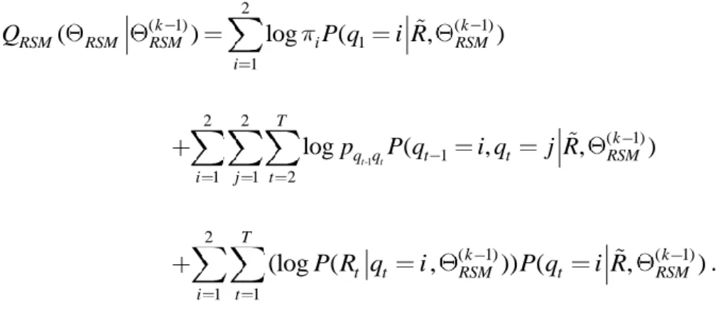
th

parameter estimates. The conditional expectation of the complete-data likelihood function, Q_RSM



_RSM _RSMk1



, can be shown as:

9 2 ( 1) ( 1) 1 1 ( k ) log ( , k ) RSM RSM RSM i RSM i Q P q i R -1 2 2 ( 1) 1 1 1 2 log ( , , ) t t T k q q t t RSM i j t p P q i q j R 2 ( 1) ( 1) 1 1 (log ( , )) ( , ) T k k t t RSM t RSM i t P R q i P q i R . (6) Next, we can use the step M to find the space of parameters that can maximize

 



k 1



RSM RSM RSM

Q    , and through Lagrange multiplier, we can finally get the estimates of ˆp₁₁, ˆp₂₂, ₁, ₂, ₁ and ₂ from the EM gradient algorithm, which can be shown as follows: ( ) ( 1) 20 ( 1) 1 10 ( 1) ( ( )) ( ) k k k k RSM RSM a d Q RSM RSM d Q RSM RSM             , (7) Here ( ) ( 1) arg max ( | ) k k RSM QRSM       , where a(0,1), 10

d _and d20 are the first

order and second order condition of QRSM



RSM RSMk 1





  with respect to _RSM .

Under the condition that QRSM



RSM RSMk 1





  is monotonically increasing, we repeat the step E and the step M until the parameter estimates converge. Then we can estimate parameters’ standard deviation by Supplemented Expectation-Maximization (SEM) proposed by Meng and Rubin (1991).

IV. Data Analysis

In this paper, we use the monthly small, large, growth, value stock as well as market indexes of MSCI European Monetary Union (EMU) from Jan. 2000 to Nov. 2012 as the sample. We obtained the monthly return data from the website of MSCI, and then calculate the market, size (SMB) and value premiums (HML) of the EMU market.

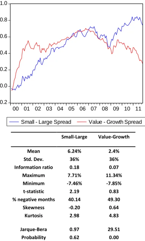
Fig. 1 shows the cumulative return distribution of the spreads and the corresponding summary statistics of MSCI European Monetary Union (EMU) for the period 2000-2011. At first glance, the value firm effect clearly lacks robustness. This is confirmed by the t-statistic in the table in Fig. 1. We fail to reject the null

10

hypothesis of a zero mean for the monthly value premium. Small stocks, on the other hand, did particularly well relative to large stocks. The information ratio of the buy-and-hold portfolio, defined as the ratio of the mean return to the standard deviation, is 0.18. The t-statistic of 2.19 indicates the value premium is significantly positive at a 5% level. The lack of robustness of the value firm effect clearly emphasizes the possible benefits of a style timing routine.

[Insert Fig. 1]

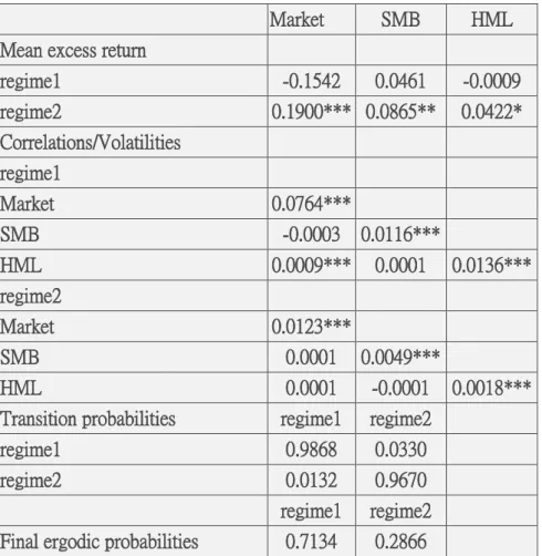
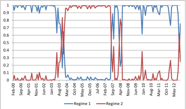
Next, we input the market, size and value premiums of the EMU market into the regime-switching model to see if there exist the style cycle in the market. The estimation results in Table 1 show that there exist two states to describe the joint return process on the market, SMB and HML portfolios. Regime 1 classifies the highly volatile bear market where only SMB has insignificantly positive return, while regime 2 is the bull market that all three portfolios have significantly positive returns. The volatilities of portfolios are higher in regime 1 (bear market) than in regime 2 (bull market). Moreover, under regime 1, the returns on the HML portfolio are positively correlated with that of the market portfolio, economically and statistically significantly. Figure 2 plots the associated filtering probabilities of state 1 and 2. The figure shows that regime 1 captures the early 2000s recession as well as the 2008 global financial crisis.

The steady state probabilities implied by the estimates of the transition matrix

ˆP are 71% and 29%, respectively. Furthermore, the transition probabilities indicate that the market more easily exits to regime 1 from regime 2 (3.3%) than vice versa (1.3%).

[Insert Table 1] [Insert Figure 2]

V. Trading strategy and empirical results

First, we set up the trading strategy. Using the filtering probability in the period t and the estimated transition probabilities, we can get the expected probability:

P(𝑠𝑡+1= 𝑗|𝐼𝑡, 𝜃) = ∑3𝑖=1P(𝑠𝑡= 𝑖|𝐼𝑡, 𝜃)∙ 𝑝𝑖𝑗 (8)

We then define the state with the largest expected probability as the expected state, and use different trading strategies with varying expected states. According to the estimation of regime-switching model in the previous section, we compute the optimal weights of the market, SMB, HML and risk free rate (R_f) portfolios by the mean-variance analysis. The mean-variance analysis indicates that in the regime 1, we

11

should put the weights of [1.15, -0.15, 0.69, 0.39] to the portfolio of [R_f, market, SMB, HML], while put the weights of [0.89, 0.11, 0.34, 0.61] to the portfolio of [R_f, market, SMB, HML] under the regime 2.

In-sample tests

Following the trading strategy mentioned above, the in-sample performance is reported in Table 2. The cumulative returns are plotted in Figure 3. From Table 2, the annual return of the trading strategy is about 8.5%, higher than the style consistent strategy, the SMB, 5.9%, and the HML, 1.3%. Moreover, from Fig. 3, we can see the cumulative return of the trading strategy is about 110%, while the SMB and the HML are only 76.3% and 19.3%, respectively.

In perspective of portfolio risk, the standard deviation of the trading strategy is smaller than the SMB and the HML portfolios, and the numbers of negative returns are less than the other two portfolios. The results indicate that the risk-adjusted return of the trading strategy is better than those of style consistent trading strategies.

[Insert Table 2] [Insert Figure 3]

Out of sample tests

In this study, we use the sample spanning from Feb. 2008 to Nov. 2012 for the out of sample tests. Therefore, the sample from Jan. 2000 to Jan. 2008 is used for model estimation. As time passes, we add new information into model estimation to deliver the precise results for investors.

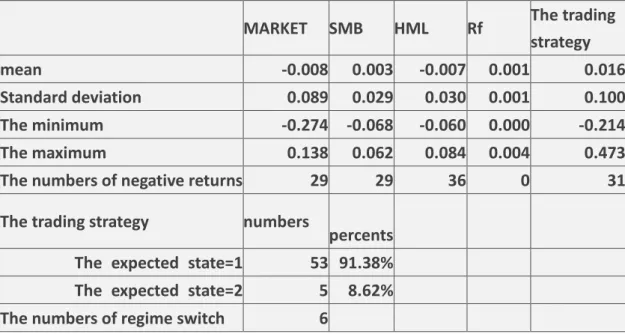
Table 3 reports the out of sample tests results. From the table, we find that the annual return of the trading strategy is about 19.6%, higher than the style consistent strategies, the SMB, 3.8%, and the HML, -8.3%. However, the standard deviation of the trading strategy is higher than the SMB and the HML portfolios, and the numbers of negative returns are more than the SMB portfolio. But the Sharpe ratios still indicate that the risk-adjusted return of the trading strategy is better than those of style consistent trading strategies.

[Insert Table 3]

VI. Conclusion

The 2008 global financial crisis induced cross-asset de-levering/sell-off, overcrowded investment strategies. The instable macroeconomic environment has resulted in abnormal style correlations and volatility, and sudden style reversals.

12

Hence, the style consistent strategies may not provide the long-term benefits often assumed in the literature. In this study, we try to build a dynamic trading strategy that can indicative to managers to switch styles.

We use the Markov regime-switching model to generate the switching signal of size and value portfolios in the stock markets in the Euro area. The results of the rotation strategies are compared with the style consistent buy-and-hold strategies. According to the in-sample and out of sample test, we find that the portfolio returns with regime shifts significantly outperforms those with style consistent strategies. In addition, the portfolio risk is reduced effectively. Therefore, accounting for regime changes in style investments is critical for investors.

References

Bauer, R., Derwall, J. and Molenaar, R., 2004. The real-time predictability of the size and value premium in Japan, Pacific-Basin Finance Journal. 12, 503–23.

Breen, W., Glosten, L. R., Jagannathan, R., 1989. Economic Significance of Predictable Variations in Stock Index Returns. The Journal of Finance 44, 1177-1189. Cooper, M., Gulen, H., Vassalou, M., 2001. Investing in size and book-to-market portfolios using information about the macroeconomy: Some new trading rules. Working Paper, Purdue University.

Engel, C., 1994. Can the Markov switching model forecast exchange rates? Journal of International Economics 36, 151-165.

Engel, C., Hamilton, J., 1990. Long swings in the dollar: are they in the data and do markets know it? The American Economic Review 80, 689-713.

Hamilton, J.D., 1989. A new approach to the economic analysis of nonstationary time series and the business cycle. Econometrica, 57, 357-384.

Levis, M., Liodakis, M., 1999. The profitability of style rotation strategies in the United Kingdom. Journal of Portfolio Management 25, 73– 86.

Manganelli, S., 2004. Asset allocation by variance sensitivity analysis. Journal of Financial Econometrics 2, 370–389.

Meng, X.L., Rubin, D.B., 1991. Using EM to obtain asymptotic variance-covariance matrices: The SEM algorithm. Journal of the American Statistical Association 86, 899-909.

Patton, A., 2004. On the out-of-sample importance of skewness and asymmetric dependence for asset allocation. Journal of Financial Econometrics 2, 130–168.

Timmermann, A., 2000. Moments of Markov switching models. Journal of Econometrics 96, 75–111.

13

Table 1: Parameter estimates of the regime-switching model for the market, SMB and

HML returns

Market SMB HML

Mean excess return

regime1 -0.1542 0.0461 -0.0009 regime2 0.1900*** 0.0865** 0.0422* Correlations/Volatilities regime1 Market 0.0764*** SMB -0.0003 0.0116*** HML 0.0009*** 0.0001 0.0136*** regime2 Market 0.0123*** SMB 0.0001 0.0049*** HML 0.0001 -0.0001 0.0018***

Transition probabilities regime1 regime2

regime1 0.9868 0.0330

regime2 0.0132 0.9670

regime1 regime2

Final ergodic probabilities 0.7134 0.2866

14

Table 2: In-sample performance comparison

MARKET SMB HML Rf The trading

strategy

mean -0.0012 0.00495 0.00111 0.00221 0.007063

Standard deviation 0.06913 0.02808 0.02858 0.00121 0.0243866

The minimum -0.2742 -0.0746 -0.0785 0.00011 -0.071504

The maximum 0.14548 0.07703 0.11344 0.00435 0.1175515

The numbers of negative

returns 71 64 77 0 54

The trading strategy

numbers percents

The expected state=1 107 69.48%

The expected state=2 47 30.52%

The numbers of regime

switch 8

Table 3: Out of sample performance comparison

MARKET SMB HML Rf The trading

strategy

mean -0.008 0.003 -0.007 0.001 0.016

Standard deviation 0.089 0.029 0.030 0.001 0.100

The minimum -0.274 -0.068 -0.060 0.000 -0.214

The maximum 0.138 0.062 0.084 0.004 0.473

The numbers of negative returns 29 29 36 0 31

The trading strategy numbers

percents

The expected state=1 53 91.38%

The expected state=2 5 8.62%

15 Small-Large Value-Growth Mean 6.24% 2.4% Std. Dev. 36% 36% Information ratio 0.18 0.07 Maximum 7.71% 11.34% Minimum -7.46% -7.85% t-statistic 2.19 0.83 % negative months 40.14 49.30 Skewness -0.20 0.64 Kurtosis 2.98 4.83 Jarque-Bera 0.97 29.51 Probability 0.62 0.00

Fig. 1 Cumulative month-to-month size and value premium. Fig. 1 shows cumulative month-to-month

small/large (value/growth) return spread during the period 2000:01 – 2012:11. The corresponding table presents summary statistics for each of the spreads. Mean values and standard deviations are presented on an annualized basis. The information ratio is the mean divided by the standard deviation. The t-statistic indicates the significance of the mean. The Jarque-Bera probability indicates the probability that the null hypothesis of a normally distributed series holds.

-0.2 0.0 0.2 0.4 0.6 0.8 1.0 00 01 02 03 04 05 06 07 08 09 10 11 Small - Large Spread Value - Growth Spread

16

Fig. 2. Filtered state probabilities of Regime 1 and Regime 2.

Fig. 3. Cumulative month-to-month returns

0 0.1 0.2 0.3 0.4 0.5 0.6 0.7 0.8 0.9 1 Fe b -00 Se p -00 Ap r-01 N o v-01 Ju n -02 Jan -03 Au g-03 Ma r-04 Oct-04 Ma y-0 5 De c-0 5 Ju l-06 Fe b -07 Se p -07 Ap r-08 N o v-08 Ju n -09 Jan -10 Au g-10 Ma r-11 Oct-11 Ma y-1 2 Regime 1 Regime 2 -1 -0.5 0 0.5 1 1.5 Fe b -00 Se p -00 Ap r-01 N ov -01 Ju n -02 Jan -03 Au g-03 Ma r-04 Oct-04 Ma y-0 5 De c-0 5 Ju l-06 Fe b -07 Se p -07 Ap r-08 N o v-08 Ju n -09 Jan -10 Au g-10 Ma r-11 Oct-11 Ma y-1 2

17

國科會補助專題研究計畫成果報告自評表

請就研究內容與原計畫相符程度、達成預期目標情況、研究成果之學術或應用價值

（簡要敘述成果所代表之意義、價值、影響或進一步發展之可能性）

、是否適合在學

術期刊發表或申請專利、主要發現（簡要敘述成果是否有嚴重損及公共利益之發現）

或其他有關價值等，作一綜合評估。

1. 請就研究內容與原計畫相符程度、達成預期目標情況作一綜合評估

X 達成目標

□ 未達成目標（請說明，以 100 字為限）

□ 實驗失敗

□ 因故實驗中斷

□ 其他原因

說明：

2. 研究成果在學術期刊發表或申請專利等情形：

論文：□已發表 □未發表之文稿 X 撰寫中 □無

專利：□已獲得 □申請中 X 無

技轉：□已技轉 □洽談中 X 無

其他：

（以 100 字為限）

18

3. 請依學術成就、技術創新、社會影響等方面，評估研究成果之學術或應用價值

（簡要敘述成果所代表之意義、價值、影響或進一步發展之可能性），如已有嚴重

損及公共利益之發現，請簡述可能損及之相關程度（以 500 字為限）

2008 年全球金融危機後，造成資產交互去槓桿化及投資策略過度壓縮。在此不穩定的經濟環境 更引發了不同特色投資組合的超常相關性和波動性，甚至特色投資的反轉現象。所以傳統的一致 化特色投資策略可能無法再提供過去文獻所引述的長期獲利。本研究將關注在規模及價值投資溢酬 的動態變化並建立一個能預警經理人反轉其特色投資策略的模型。我們將使用馬可夫狀態轉換模型 去預測歐元區的股票市場規模及價值風險溢酬的方向變動，進而提供經理人買賣投資組合的訊息。 透過將樣本期間區分為兩種情境，根據各情境特性決定相對應之最適資產配置，並以預期情境轉換 機率決定投資組合調整時機，模擬投資人在現有可得資訊下所做的投資決策以檢定此投資策略是否 能提升特色一致投資交易者的投資績效。根據樣本外實證測試結果，考慮情境因子的模擬投資策略 之報酬優於特色一致交易策略，且可有效降低風險，顯示納入情境因子的考量有助提升資產配置效率 ，藉由預期下一期的情境可使進行特色交易的投資人具備擇時機會，幫助預測未來景氣走勢並於空頭 市場時承擔較低的風險並獲得相對優異的風險調整後報酬。

19

國科會補助專題研究計畫出席國際學術會議心得報

告

日期： 年 月 日

計畫編號

NSC

101-2410-H-004 -053 –

計畫名稱

使用狀態轉換模型進行特色反轉投資策略

在歐洲區規模及價值風險溢酬的研究

出國人員

姓名

林建秀

(由於懷孕生

產，故無法出

國開會)

服務機

構及職

稱

政治大學金融系

會議時間

年 月 日

至

年 月 日

會議地

點

會議名稱

(中文)

(英文)

發表題目

(中文)

(英文)

國科會補助專題研究計畫出席國際學術會議心得報

告

日期： 年 月 日

計畫編號

NSC

101-2410-H-004 -053 –

計畫名稱

使用狀態轉換模型進行特色反轉投資策略

在歐洲區規模及價值風險溢酬的研究

出國人員

姓名

林建秀

(由於懷孕生

產，故無法出

國開會)

服務機

構及職

稱

政治大學金融系

會議時間

年 月 日

至

年 月 日

會議地

點

會議名稱

(中文)

(英文)

發表題目

(中文)

(英文)

國科會補助計畫衍生研發成果推廣資料表

日期:2014/02/25

國科會補助計畫

計畫名稱: 使用狀態轉換模型進行特色反轉投資策略在歐洲區規模及價值風險溢酬的研究 計畫主持人: 林建秀 計畫編號: 101-2410-H-004-053- 學門領域: 財務

無研發成果推廣資料

101 年度專題研究計畫研究成果彙整表

計畫主持人：林建秀 計畫編號： 101-2410-H-004-053-計畫名稱：使用狀態轉換模型進行特色反轉投資策略在歐洲區規模及價值風險溢酬的研究 量化 成果項目 實際已達成 數（被接受 或已發表） 預期總達成 數(含實際已 達成數) 本計畫實 際貢獻百 分比 單位 備 註 （ 質 化 說 明：如 數 個 計 畫 共 同 成 果、成 果 列 為 該 期 刊 之 封 面 故 事 ... 等） 期刊論文 0 0 100% 研究報告/技術報告 0 0 100% 研討會論文 0 0 100% 篇 論文著作 專書 0 0 100% 申請中件數 0 0 100% 專利 已獲得件數 0 0 100% 件 件數 0 0 100% 件 技術移轉 權利金 0 0 100% 千元 碩士生 2 4 100% 博士生 2 0 100% 博士後研究員 0 0 100% 國內 參與計畫人力 （本國籍） 專任助理 0 0 100% 人次 期刊論文 0 0 100% 研究報告/技術報告 0 0 100% 研討會論文 1 1 100% 篇 論文著作 專書 0 0 100% 章/本 申請中件數 0 0 100% 專利 已獲得件數 0 0 100% 件 件數 0 0 100% 件 技術移轉 權利金 0 0 100% 千元 碩士生 0 0 100% 博士生 0 0 100% 博士後研究員 0 0 100% 國外 參與計畫人力 （外國籍） 專任助理 0 0 100% 人次

其他成果

(

無法以量化表達之成 果如辦理學術活動、獲 得獎項、重要國際合 作、研究成果國際影響 力及其他協助產業技 術發展之具體效益事 項等，請以文字敘述填 列。) 無 成果項目 量化 名稱或內容性質簡述 測驗工具(含質性與量性) 0 課程/模組 0 電腦及網路系統或工具 0 教材 0 舉辦之活動/競賽 0 研討會/工作坊 0 電子報、網站 0 科 教 處 計 畫 加 填 項 目 計畫成果推廣之參與（閱聽）人數 0

國科會補助專題研究計畫成果報告自評表

請就研究內容與原計畫相符程度、達成預期目標情況、研究成果之學術或應用價

值（簡要敘述成果所代表之意義、價值、影響或進一步發展之可能性）

、是否適

合在學術期刊發表或申請專利、主要發現或其他有關價值等，作一綜合評估。

1. 請就研究內容與原計畫相符程度、達成預期目標情況作一綜合評估

■達成目標

□未達成目標（請說明，以 100 字為限）

□實驗失敗

□因故實驗中斷

□其他原因

說明：

2. 研究成果在學術期刊發表或申請專利等情形：

論文：□已發表 □未發表之文稿 ■撰寫中 □無

專利：□已獲得 □申請中 ■無

技轉：□已技轉 □洽談中 ■無

其他：（以 100 字為限）

3. 請依學術成就、技術創新、社會影響等方面，評估研究成果之學術或應用價

值（簡要敘述成果所代表之意義、價值、影響或進一步發展之可能性）（以

500 字為限）

2008 年全球金融危機後，造成資產交互去槓桿化及投資策略過度壓縮。在此不穩定的經 濟環境更引發了不同特色投資組合的超常相關性和波動性，甚至特色投資的反轉現象。所 以傳統的一致化特色投資策略可能無法再提供過去文獻所引述的長期獲利。本研究將關注 在規模及價值投資溢酬的動態變化並建立一個能預警經理人反轉其特色投資策略的模 型。我們將使用馬可夫狀態轉換模型去預測歐元區的股票市場規模及價值風險溢酬的方向 變動，進而提供經理人買賣投資組合的訊息。透過將樣本期間區分為兩種情境，根據各情 境特性決定相對應之最適資產配置，並以預期情境轉換機率決定投資組合調整時機，模擬 投資人在現有可得資訊下所做的投資決策以檢定此投資策略是否能提升特色一致投資交 易者的投資績效。根據樣本外實證測試結果，考慮情境因子的模擬投資策略之報酬優於特 色一致交易策略，且可有效降低風險，顯示納入情境因子的考量有助提升資產配置效率， 藉由預期下一期的情境可使進行特色交易的投資人具備擇時機會，幫助預測未來景氣走勢 並於空頭市場時承擔較低的風險並獲得相對優異的風險調整後報酬。