利用等位函數法結合形狀資訊做影像序列的物體追踪

(1)

國立交通大學

資訊工程學系

碩士論文

利用等位函數法結合形狀資訊做影像序列的物體追

踪

Object Tracking via the Level Set Method Integrated

with Prior Shape

研究生：徐錦祥

指導教授：陳稔博士

(2)

利用等位函數法結合形狀資訊做影像序列的物體追踪

Object Tracking via the Level Set Method Integrated with

Prior Shape

研究生：徐錦祥 Student：Chin-Hsiang Hsu 指導教授：陳稔 Advisor：Zen Chen 國立交通大學資訊工程學系碩士論文 A Thesis

Submitted to Department of Computer Science and Information Engineering College of Electrical Engineering and Computer Science

National Chiao Tung University in Partial Fulfillment of the Requirements

for the Degree of Master

in Computer Science and Information Engineering July 2005

Hsinchu, Taiwan, Republic of China

(3)

利用等位函數法結合形狀資訊做影像序列的物體追踪

學生：徐錦祥指導教授：陳稔博士

國立交通大學資訊工程學系

摘要

物體追踪在電腦視覺、監測系統、交通監測站等，都有很大的應用，並且提供了高階影像處理的前置工作。本論文提出一個對影像序列的物體輪廓線追踪方法。主要是結合物體形狀資訊來改進 Abdol-Reza Mansouri 的方法。在 Abdol-Reza 的方法中，追踪演算法主要是透過最小化一個由貝氏定理所推導出的能量函數，來變動所要用來追踪的輪廓線，使其往目標物逼進。此方法有三個優點。第一，不需要做物體運動估測。第二，物體允許任意變形，包括拓樸的改變。第三，物體的輪廓梯度不需要很大。而它所面臨的缺點是，當物體的附近有跟其相近的背景時，追踪的結果將會受到很大的影響。我們希望透過結合物體的形狀資訊來改進這個缺點。當被追踪物體有部分跟背景相似時，明確的部分由原來的方法追踪，並將其結果與形狀資訊對齊，接著由形狀資訊將不明確的部分補足。如果物體本身就整個能與背景分開時，形狀資訊的權重將會自動被付予很小的值，以保有物體允許隨意變形的特性。這樣的整合方式，也將使我們的方法更具有彈性。

(4)

Object Tracking via the Level Set Method Integrated

with Prior Shape

student

：

Chin-Hsiang Hsu

Advisor

：Dr. Zen Chen

Department of Computer Science and Information Engineering

National Chiao Tung University

Abstract

Detecting and tracking moving objects has a wide variety of applications in computer vision such as computer vision, video surveillance, traffic monitoring, etc. Additionally, it provides input to higher level vision tasks. This thesis presents an approach to tracking a moving object over a sequence of images. In particular, we improve the Abdol-Reza’s model by coupling with shape prior knowledge for shape perseverance in case of ambiguity.

In the model of Abdol-Reza, tracking is achieved by evolving the contour from frame to frame by minimizing an energy functional evaluated by Bayesian theory. There are three two favorable features in this model. First, no motion field or parameters needed to be computed. Second, deformable shapes of the object are allowed and the topology of the boundary is not constrained. Third, no assumption is made on the strength of the edge gradient. However, it also suffers from the

constraints imposed on a degree of dissimilarity between the object and the background. A background region similar to the object might corrupt the contour evolution. We want to overcome this drawback by coupling with a shape prior in the

(5)

associated energy functional. When the object is partially involved in a similar

background, the original tracking term in the functional will dominate the result in the unambiguous background part, and the prior shape will guide the object movement in the ambiguous part. If the object is entirely distinguishable from the background, the weight of the shape prior is set low and thus allowing free deformation of the object. Compared to other tracking methods embedded with shape priors, the presented approach is more flexible, retaining the advantage of suffering little constraints on the deformable shape of the tracked object in many cases.

(6)

誌謝

首先要感謝陳稔教授兩年來的悉心教導，這段期間培養出我

獨立思考的能力，在學習態度、研究方法上也得到長足進步。每每在

研究過程中遭遇困難時，老師總能積極給予幫助。因為有來自老師的

援助，這篇論文才得以順利完成，在此向老師獻上無盡的謝意。

其次我要感謝許志宇學長在這期間曾經給我的指導。您犧牲晚上

及假日休閒的時間給我細心的建議及教導，使我得以一窺等位函數法

的堂奧，並在研究方法上有所突破。這篇論文的完成，您真的給我很

大的幫助，在此我要由衷的感激您!

感謝實驗室全體的成員，方彥翔學長，顧正偉同學、朱佑吾同學、

紀文原同學、蘇永迪同學、陳柏聰學弟、鄭龍凱學弟、吳昶浩學弟。

您們都曾在研究期間給予意見，並給予我許許多多的幫助，謝謝你們

陪我走過這一段日子。

感謝我的父母親及親愛的家人，你們無怨無悔的支持與付出，讓

我能全心全意關注我的研究，在生活上無後顧之憂。你們所給我精神

上的支持與鼓勵，這一切都是使我能義無反顧向前邁進的動力。

感謝我的好朋友建勳。在遭遇困難時，我們彼此互相鼓勵，這是

促使我繼續努力的動力。

當然我還要感謝其他許許多多的朋友。紙短情深，在此無法一一

致謝，僅以本篇論文獻給你們，再次說聲謝謝！

徐錦祥於交大

(7)

List of Figures

Fig 4.1 Idea of Abdol-Reza’s model ...13

Fig 4.2 Discriminate analysis...15

Fig 4.3 Level set representation ...17

Fig 4.4 The camouflage synthetic sequence ...19

Fig 4.5 Problem of Abdol-Reza’s model...20

Fig 4.6 Approximation of F∆t ...21

Fig 4.7 Numerical Problem...22

Fig 4.8 Bubble effect...23

Fig 5.1 Image energy and Shape energy ...27

Fig 5.2 Gradient vector ...28

Fig 5.3 Shape and its forces field...29

Fig 5.4 Shape prior illustration 1 ...33

Fig 5.5.Shape prior illustration 2 ...34

Fig 6.1 Abdol-Reza’s model ...40

Fig 6.2 Abdol-Reza’s model + shape prior ...40

Fig 6.6 Abdol-Reza’s model + Shape prior...42

Fig 6.7 Abdol-Reza’s model. ...43

Fig 6.9 Abdol-Reza’s model. ...44

Fig 6.11 Abdol-Reza’s model...44

Fig 6.13 Abdol-Reza’s model + Shape prior + Background removal...45

Fig 6.14. Abdol-Reza’s model.on digital camera photos ...46

Fig 6.15. Abdol-Reza’s model + shape prior on digital camera photos...47

Fig 6.16 Mechanism of shape prior ...48

Fig 6.19 Two hands, with shape prior model...51

Fig 6.20 Two hands, Abdol-Reza’s model ...52

(9)

Fig 6.23 Human ...55

Fig 6.24 Initial contour ...57

Fig 6.25 α = 500...58 Fig 6.26 α = 1000...59 Fig 6.27 α = 1500...61 Fig 6.28 α = 2000...62 Fig 6.29 α = 2500...63 Fig 6.30 α = 3000...64 Fig 6.31 α = 3500...65 Fig 6.32 α = 4000...66 Fig 6.33 λ =0.01 ...68 Fig 6.34 λ =0.03 ...69 Fig 6.35 λ =0.05 ...70 Fig 6.36 λ =0.07 ...71 Fig 6.37 λ =0.09 ...72 Fig 6.38 λ =0.11 ...73 Fig 6.39 λ =0.13 ...74

(10)

1. Introduction

1.1. Motivation

High level vision tasks for video processing require tracking of the complete contour of the objects, such as in the applications of computer vision such as computer vision, video surveillance, traffic monitoring, etc.

1.2. Object Tracking

Numerous approaches for tracking objects in an image sequence are proposed and can be mainly classified in three categories:

1. Correspondence-based object tracking: Tracking is performed by establishing correspondence of the objects in consecutive frames. These approaches rely on the detection of temporal changes and employ a thresholding technique over the inter-frame difference. These methods can only be applied to images with static backgrounds and they provide coarse object silhouettes.

2. Motion-based object tracking: Tracking is performed by estimating the motion of objects in consecutive frames. Objects are represented by planar surfaces, such as rectangle and ellipse, or their centroids. These methods are relatively fast but have considerable difficulties in dealing with non-rigid movements and objects. 3. Model-based object tracking: Object representation includes rigid models and

non-rigid models, or deformable templates. Such models usually have a number of parameters to control the shape and pose of the model. These methods suffer from high computational costs for complex models due to the need for coping

(11)

with scaling, translation, rotation and deformation.

In correspondence-based object tracking, background subtraction is the most popular detection method used in object trackers, where color observations of individual pixels in a reference frame are statistically modeled. Detection is performed by labeling the pixels that deviate from the static model.

In motion-based tracking, a statistical analysis is performed and is used to provide the motion-based estimation. Motion models used are translation, scaling and affine motion models. One of the most common motion based tracker is “template matching”, where translation of an object template is computed by searching the image for a similar template. Additionally, by assuming a smooth background, the input frame can be used directly to provide an accurate object tracking result.In [8], the authors proposed a kernel-based tracker in which color priors are computed using weighted kernel density estimation. Mean-shift vector is then computed iteratively by maximizing likelihood between the object color prior and the model generated from hypothesized object position.

There is a substantial use of flexible models or deformable templates in model-based tracking. There are three broad classes of these models.

(i) Articulated models: Articulated models are built up from a number of rigid components connected by sliding or rotating joints. This approach is only applicable to a restricted class of variable shape problems.

(ii) Statistical models of shape: The shape is represented by a set of boundary points connected by arcs with a statistical model of relationships between them, or a set of points with distributions related by a covariance matrix. (iii) Active contour models: There are two general types of active contour

(12)

models in the literature today: parametric active contours (snakes) [1] and geometric active contours [2][4]. Parametric active contours, or snakes, can be considered as parameterized models, or the parameters being spline control points. The idea of fitting is minimization of an energy functional to apply forces to the model. In recent years, it is popular to represent

parametric active contour by geometric active contours such as one of the level sets in higher dimensional space.

This thesis presents an approach for contour tracking formulated as a calculus of variations problem. The proposed energy functional contains two energy terms, the image energy Er and the shape energy Es. Image energy, which is based on a

Bayesian framework [17], performs discriminate analysis on pixels. The shape energy, motivated from the geodesic active contour model [2], is weighted by confidence of the decrease of the image energy and resolve discriminate uncertainties. Tracking is achieved by evolving the contour, which is represented using level sets, to a position in the gradient descent direction of the energy functional. Also, invariance to

transformations of shape energy is achieved by minimize a pseudo distance [22] between the evolving contour and the shape model.

1.3. Thesis Organization

This thesis is organized as follows. The following chapter contains a review of related work. Chapter 3 describes the problem investigated in this thesis. In Chapter 4, we introduce Abdol-Reza’s model for tracking and present its drawback. Level set implementation issues are also briefly discussed. Then the shape prior solution is described in chapter 5, together with extension of our method. Finally, the thesis ends with several experimental results in chapter 6 followed by conclusions in chapter 7.

(13)

2. Related Work

2.1. Active Contour Models

Since active contour was introduced to the vision community by Kass et al. (1988), extensive researches was done on “snakes” or parametric active contour models for boundary detection. The classical approach is based on deforming an initial contour towards the boundary of the object to be detected. The deformation is obtained by trying to minimize a functional designed such that its minimum is

obtained at the boundary of the object. The energy functional is basically composed of two components, one controls the smoothness of the curve and another attracts the curve towards the boundary. However, there are three key difficulties with parametric active contour algorithms. First, the initial contour must be close to the true boundary or it will likely converge to the wrong result. Then, active contours have difficulties progressing into boundary concavities. Finally, energy model is not capable of handling changes in the topology of the evolving contour when direct

implementations are performed. An approach insensitive to initialization and the ability to move into boundary concavities is proposed in [1]. The author present external forces originate from an edge map of the image to provide larger capture range. However, this parametric model cannot handles topology changes as well.

Recently, novel geometric models of active contours were proposed [2] [4]. These models are based on the theory of curve evolution and geometric flows, which has received a large amount of attention in recent years. It allows automatic changes in the topology when implemented using the level-sets based numerical algorithm

(14)

[6][7]. Thereby, several objects can be detected simultaneously without previous knowledge of their number in the scene and without using special tracking procedures.

However, because the flow may be slow to converge in practice, a constant term is added to keep the curve moving in the desired direction. Kaleem et al. [10] modify this term based on the gradient flow derived from a weighted area functional, with image dependent weighting factor. Since this flow requires the computation of only first order derivatives, it offers significant computational savings over the weighted length minimizing flow.

Active contour models that rely on the edge-detector or image gradient can detect only objects with edges defined by gradient. In practice, the discrete gradients are bounded and then the stopping function is never zero on the edges, and the curve may pass through the boundary. Chan and Vese detailed a level set implementation of the Mumford-Shah functional [9], which is based on the use of the Heaviside function as an indicator function for the separate phases. The idea is to partition the given image into two homogeneous regions, without a stopping edge-detector. The authors also extend this binary image oriented method to segment images with more than two regions by multiphase level sets [12].

To segment objects in textured background, Paragios and Deriche proposed a region-based energy, where statistical models were used for textured object and background regions [16]. They extended the region model to the mixture of Gaussians for magnitude of Gabor filter responses. The texture segmentation is obtained by unifying region and boundary-based information.

(15)

the image frames history. If the contour is initialized with its previous position, contour segmentation approaches become object trackers, and tracking is defined based on motion information to evolve an initial object contour[4][14][17][18][19].

In [4], the evolution equation for contour is obtained by image differences, this tracking algorithm can be applied only when an important degree of similarity among the images and displacements involved are small. G. Tsechpenakis et al. proposed a method handling the appearance of occlusions between different objects [19]. The use of the object motion history and statistical measurements provide information for the extraction of uncertainty regions. In [14], tracking is expressed as detection and tracking of moving objects in image sequences. In the proposed algorithm, a detection step forces a closed curve to converge towards moving areas of an image, while a tracking step evolves the curve to coincide with the exact boundary of the moving object. The tracking step is only an intensity boundary detection algorithm using active contours and implemented using level sets. Since the tracking step relies on the previous frame, the background is assumed to be stationary. The problem addressed in [17] is that object tracking can be treated as two-class discriminate analysis of pixels, where the classes correspond to the object and the background regions. Since his approach compute for each pixel by brute-force search in a circular neighborhood, there are two problems exist even when strong assumption on intensity boundaries. First, the contour cannot capture the parts of the object near where existing a background region with similar intensities to them. The second, the background around the contour will be classified as the object if there exist some pixels with similar intensities within the object. The classification criterion is extended in [18]. A window of specified fixed size is defined for each pixel around the contour. The contour will move in the direction that can equalize the numbers of pixels within the

(16)

window that belong to two classes (object and background). Also, shape priors are used to recover the missing object regions during occlusion. Nevertheless, since the shape prior takes effect only when the occlusions are detected, this approach still suffers the problems as encountered by [17].

Our approach is the incorporation of knowledge about the shape with [2], to control the difficult conditions of the image. However, different from[18], we improve the tracking results of [17] instead of handling occlusions of the objects.

2.2. Shape Priors

In the substantial literature of deformable models, there are three main

mechanisms can be found to constraint the shape of the curve during the evolution of the deformable model:

1. Free-form approaches: These methods do not encode a default shape, but the energy functional imposes smoothness and compactness of the boundary of the surface. They can be seen as general, weak and local shape constraints.

2. Analytical parametric templates: The analytical shape constraints are defined by the distribution of the admissible parameters. These methods are commonly used when some prior information about the geometrical shape is available, which can be encoded using a small number of parameters.

3. Prototype-based constraints: Shapes are represented by the mean shape of a collection of individuals and their statistical variations. These methods require either training or global shape modeling.

T. F. Cootes et al. propose a method that uses point distribution model (PDM) [13] as the prototype-based constraints. It describes the average and characteristic shape variations of a set of training samples, which are given in the form of a set of points on the learning boundaries. In [21], the authors investigate the use of discrete cosine transform (DCT) coefficients in describing object shape. The method starts

(17)

with local shape parameterization, then, the shape is converted into an implicit representation using global shape parameters. As can be seen, incorporating prior shape information in a deformable model, requires either training or global shape modeling. Training involves manual interaction to accumulate information on the shape variability of the

same object class. Global modeling can be characterized using only a few parameters, and tend to be much more stable than local properties. The choice of a certain shape representation determines to a great extent the flexibility, processing speed, and amount of user interaction.

Leventon et al. [23] have incorporated statistical shape information into the evolution of geodesic active contours. They compute a prior on shape variation given a set of training instances. Each curve in the training dataset is embedded as the zero level-set of three-dimensional surface, which is a signed distance function. Daniel Cremers et al. [22] propose a closed-form, spline based solution for incorporating invariance with respect to similarity transformations in the variational framework. Dainiel Cremers and Stefano Soatto [20] integrate prior shape knowledge into level set based segmentation methods and proposed dissimilarity measures for shapes encoded by the signed distance function.

The proposed shape prior is a global shape model using the initial contour as the shape prior but not the training set from the image history, therefore the number of parameters involved can be reduced. It is motivated by modeling the flow field of the shape forces as geodesic active contours [23], incorporating invariant transformation by the pseudo distance measure [22] and alternatively computing the total energy and the shape energy during the evolution of the curve.

(18)

3. Overview of the Proposed

Approach

Given an image sequence with a specified object and its boundary in the first frame, the thesis is to identify the boundary in all the image sequence. We use level set model to represent the curve that used to capture the object boundary. Two favorable features of level set method are its automatically handling of topology changes and easy implementation. The formula to propagate the curve is an

Euler-Lagrange equation derived from an energy functional. One of two terms in the energy functional is related with the image information and the other is for shape preserving. To solve the Euler-Lagrange equation means to minimize the energy functional and to move the curve towards the object boundary. The idea is to classify each pixel in the image as the member of the object or that of the background. If the classification is uncertain, the shape preserving term will attempt to preserve the shape of the curve and will lead the decision.

The tracking system is presented in the following flow chart:

The detailed algorithm of the presented approach is showed in the following Specify object in the 1st frame Image sequence Tracking Image sequence with object contours Video

(19)

(20)

Start

Read in the 1st image and set it as the current frame

Identify the object to be tracked and its contour

Construct the distance function of the contour in the previous frame and set it as the initial contour Generate the shape prior from the initial contour

Align the shape prior to the contour

Propagate the contour to capture the object in the current frame using the information in the previous frame and the shape prior

Is the stop condition satisfied?

N

Is there any other image frame?

Set the current image as the previous frame and set the next image as the current frame

Read in the next image

Y

N

(21)

Our approach combines three models: 1. Abdol-Reza’s model.

2. Geodesic active contour model. 3. Pseudo distance measure.

(22)

4. The Tracking Method

This chapter takes an overview of Abdol-Reza’s model. Then we point out its drawbacks in section 4.2. Finally, the implementation issues of level set method are also presented.

4.1. Abdol-Reza Mansouri’s Model

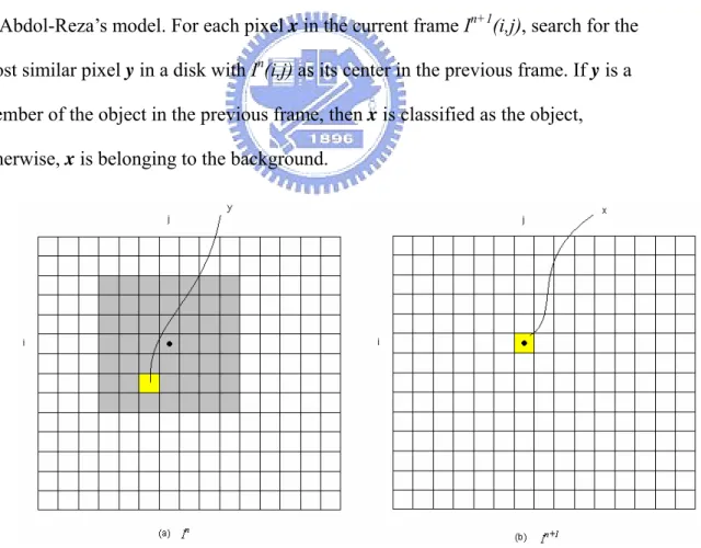
Object tracking can be treated as two-class discriminate analysis of pixels, where the classes correspond to the object and the background regions. This is also the idea of Abdol-Reza’s model. For each pixel x in the current frame In+1(i,j), search for the

most similar pixel y in a disk with In(i,j) as its center in the previous frame. If y is a

member of the object in the previous frame, then x is classified as the object, otherwise, x is belonging to the background.

Fig 4.1 Idea of Abdol-Reza’s model The shadow part is the search window.

(23)

Why this classification method works properly in Abdol-Reza’s model is because it uses level set representation for the contour model. Level set representation can divide pixels into two classes by discriminate them as either inside or outside the contour and processes only the pixels near the contour, neglecting those far away. Without this mechanism, the classification result might be a collection of

discontinuous pixels, instead of an entire object.

We now go through the approach of Abdol-Reza’s model. Let Ik be a sequence of images with domain Ω (an open subset of R2). Let R₀ ⊂Ω be a region in the n-th image (In) and be the corresponding region in image In+1 that we want to

estimate. And let

Ω ⊂ 1 R ) ( , ] 1 , 0 [ : 2 _s _γ _s

γr →ℜ _a r be a closed curve, oriented

counterclockwise, that we estimate for the boundary ∂R₁of R1. Given In, In+1 and R0,

the optimizing estimate R of R1 is found by minimizing the energy functional

ds s d R I I P d R I I P R I I E c R n n out R n n in n n r

∫

∂ ∂ + − − = + + + 1 0 0 1 , 0 1 , 0 1 ) , ) ( ( log ) , ) ( ( log ) , , ( γ λ γ r r x x x x _x x (4.1)

The first two terms on the right hand side of the functional are the external forces introduced by the image information. The first term means, given In, R0 and x belongs

to R1, the probability that x has the observing intensity In+1 (x) . Since we have the

prior of the object R0 in the previous frame, the probability is high if In+1 (x) is similar

to the intensity of some y in R0; and it is low if x is dissimilar to any pixel in R0. In

other hand, the second term means, given In, R0 and x dose not belong to R1, the

probability that x has the observing intensity In+1 (x). The probability is high if In+1 (x)

is dissimilar to any pixel in R0, otherwise, the probability is low. Using these two

(24)

by the contour. According to subtraction of these two terms, the evolving speed could be either positive or negative which indicates shrinking or expanding of the contour at that point. The other two terms are the internal force associated with the contour and will cause the contour to be smoother. Finally, the definition of the probability functions will be detailed later.

In order to minimize (1) we search for the gradient descent direction of (4.1), which can be computed from its Euler-Lagrange equation:

[

]

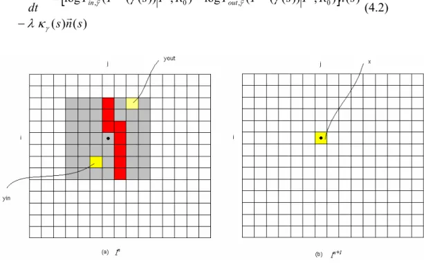
) ( ) ( ) ( ) , )) ( ( ( log ) , )) ( ( ( log ) ( 0 1 , 0 1 , s n s s n R I s I P R I s I P dt s d n n out n n in r r r r r r r γ γ γ κ λ γ γ γ − − = + + (4.2)

Fig 4.2 Discriminate analysis

The red parts represent the contour. Pin is color difference between x and yin and Pout is color difference

between x and yout. The subtraction between Pin and Pout can determine x as which class.

Then, equation (4.2) can be solved numerically by discretizing the interval on which γr is defined, leading to an explicit representation of γr . A better alternative is to represent the curve γr implicitly by the zero-level set of a function _u_:ℜ2 →ℜ.

(25)

contour representations are its independence of a particular parameterization, and the fact that the topology of the boundary is not constrained, such that merging and splitting of the contour during evolution is facilitated.

Since γr obeys an evolution equation and the zero-level set of u is assumed to coincide with γr , u must evolve according to a certain evolution equation related to that of γr . We can thus embed u in a one-parameter family and construct the

evolution equation that the zero-level set of u satisfy the evolution equation of γr .

4.2. Level Set Representation

If the evolution of γr is described by the equation ) , ( )) , ( ( ) , ( t s n t s F dt t s dγr _γ_r _r =

where F is a function defined on , the corresponding evolution of u is given by: 2 ℜ ) , ( ) ( ) ( ) ( ) ( ) ( t u F u n F y u x u t y t x t y y u t x x u t u T x x x x x x ₌ _⋅_∇ ₌ _∇ ⎥ ⎦ ⎤ ⎢ ⎣ ⎡ ∂ ∂ ∂ ∂ ⎥⎦ ⎤ ⎢⎣ ⎡ ∂ ∂ ∂ ∂ = ∂ ∂ ∂ ∂ + ∂ ∂ ∂ ∂ = ∂ ∂ _r

Since )γr( ts, is a vector in , it can be represented by a point x in the domain of u, and 2 ℜ )) , ( ( s t

F γr thus can be replaced by F(x) , leading the evolution of γr to the above equation. The condition of this correspondence is that all the points of the curve

) , ( ts

γr must be on the same level set which is the zero-level set (the set with u = 0) in most cases.

(26)

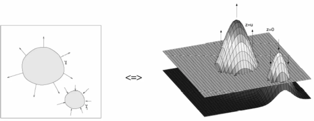
Fig 4.3 Level set representation

This figure is cut from [17]. The figure shows the equivalence between the evolution of curves γr₁,γr₂, and the evolution of function u.

Then, the level set evolution equation corresponding to the curve evolution (4.2) for tracking is given by:

[

]

u s u R I I P R I I P t u u n n out n n in ∇ − ∇ − = ∂ ∂ + + ) ( ) , ) ( ( log ) , ) ( ( log ) ( 0 1 , 0 1 , λκ x x x x x (4.3) where 2 1 } , : { 0 1 , 2 1 } , : { 0 1 , )) ( ) ( ( inf ) , ) ( ( log )) ( ) ( ( inf ) , ) ( ( log 0 0 z I I R I I P z I I R I I P n n R z z z n n out n n R z z z n n in c − + ≈ − + − ≈ − + ∈ + ≤ + + ∈ + ≤ + x x x x x x x x x x η η 2 3 2 2 2 2 ) ( 2 y x x yy xy y x y xx u _u _u u u u u u u u u u + + − = ∇ ∇ ⋅ ∇ = κ

4.3. Problems of the Abdol-Reza

Mansouri’s Model

There are two problems in the model of Abdol-Reza. First, the contour cannot capture the parts of the object near which existing a background region with similar

(27)

intensities to them. The second, the background around the contour will be classified as the object if there exist some pixels with similar intensities to them within the object. These two problems exist even in cases that objects in the images have strong intensity boundaries.

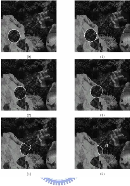
Fig 4.4 is derived from Abdol-Reza’s work [17] and shows the limits of his approach. The image sequence is constructed by cutting out a disc-like shape from the center of the image and pasting it so as to create apparent motion from the lower left corner to the upper right corner of the image. The tracking is correct until in frame 4 of the sequence, the right side of the tracked region is strongly deformed. This is due to the fact that the region and background textures are so similar there that the probability estimates Pin and Pout are almost identical for most of those pixels.

(28)

Fig 4.4 The camouflage synthetic sequence

This figure is derived from [17]. The tracked object is cut from the texture in the center of the image and pasted to create animation from the lower left corner to the upper right corner of the image.

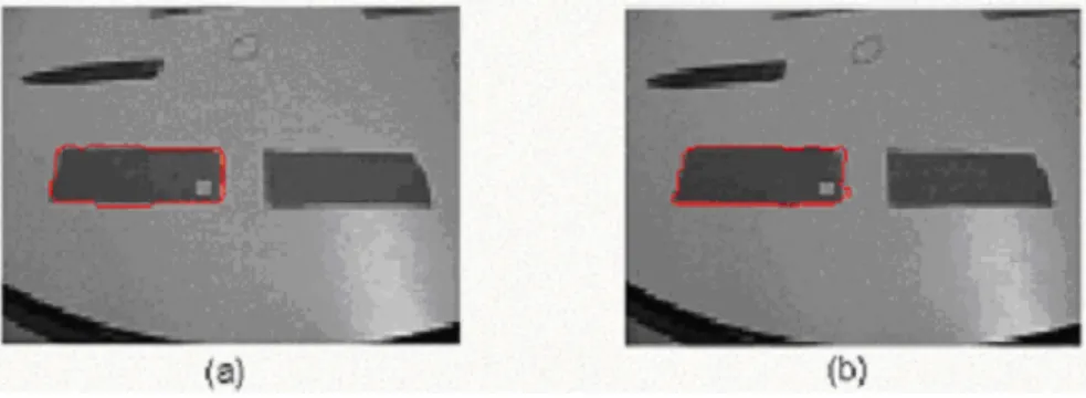
In Fig 4.5, the lower right corner of the object in frame (a) is pasted by a square shape cut from the background around the object. Then frame (a) is duplicated to create frame (b) and is applied by some noise to its background such that the background in frame (b) is more similar to the square shape than the background in frame (a). The contour is initialized in frame (a) to properly capture the object. After evolution, the lower right corner of the contour sticks out and attempts to include the background, as shown in frame (b). This is because that the background is so similar to the square shape of the object that the probability estimates are almost identical for

(29)

those pixels.

Fig 4.5 Problem of Abdol-Reza’s model

The lower right part of the contour sticks out and tries to include the background (b), due to the similarity between the background and the square shape in the object.

4.4. Implementation Issues of the

Level Set Method

The conversion from parametric representation of a curve to level set

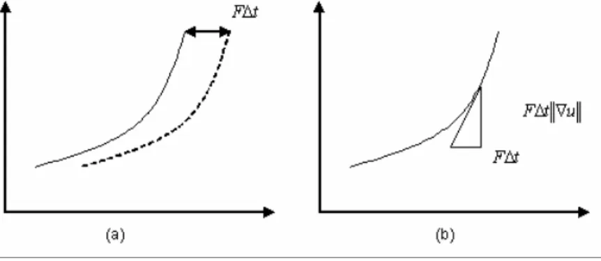
representation is exactly correct when the zero level set that representing the curve moves with a specified speed after updates of u. However, this is usually not true since the update of u is just an estimation derived from the level set equation, making some errors to the update. For example, consider an 1D curve represented by 2D level sets u, as shown in Fig 4.6(a). A perfect expression of the curve to move right with a speed F is to imaginarily move the level sets u to right with a distance , that is, to update each grid of u with the value below it after the imaginary movement, then each level set must move right with a speed F, including the level set which indicates the curve. However, this naïve kind of update is almost impossible in the real world. The update is actually an approximation derived by the level set equation, which is an increasing or decreasing amount

t F∆

u t

(30)

estimation of update of u is not correct since the level set on the new u cannot reflect the move with specified speed. And, if the function u(x) is a straight but not horizontal line on the plot, the estimation is correct and will match the imaginary movement. Also, this assumption is not useful in practice, except in very simple cases.

Fig 4.6 Approximation of F∆t

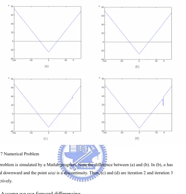
To explain it more clearly, let us take an extreme case as the example, the numerical problem when derivatives are not defined on the points that are

discontinuous. Let u be a distance function with distance from the original, that is ,

1 =

∇u everywhere except the original, as shown in Fig 4.7(a). Recall the level set equation: 0 ) , ( ) ( ) ( = ∇ + ∂ ∂ t x u x F t x u Let ⎩ ⎨ ⎧ _> _> > ≤ = ,M N 0 a x N a x M x F )(

Then, at iteration 1, u becomes Fig 4.7(b). Since for all x, F(x) > 0, each grid of u moves downward. Also, because M > N, the grids u(x≤a) moves more amount than the grids , and there is a discontinuity

occurs at u(a).

) (x a

(31)

Fig 4.7 Numerical Problem

This problem is simulated by a Matlab program. Note the difference between (a) and (b). In (b), u has moved downward and the point u(a) is a discontinuity. Then, (c) and (d) are iteration 2 and iteration 3 respectively.

Assume we use forward differencing

x u u u i i ∆ − = ∇ +1

where the lower script denotes the grid index. Then,

1 ) ( ) ( 1 ) ( ) ( ) ( ) ( ) ( 1 ) ( ) ( ) ( > ∆ − ∇ > ∇ ∴ ∆ + = ∆ − + ∆ + = ∆ − ∆ + = ∇ = ∆ ∆ − − = ∆ − ∇ x a u a u x x a u x a u x a u x a u a u x x a u a u x a u δ δ

That is, from the level set equation, will move downwards more than at iteration 2, as shown in Fig 4.7(c). If we compute iteratively in this

) (a u ) (a x u −∆

(32)

manner, will touch the x-axis to become the member of the zero level set that represents the curve and produce a “bubble effect”, as shown in Fig 4.8.

) (a u

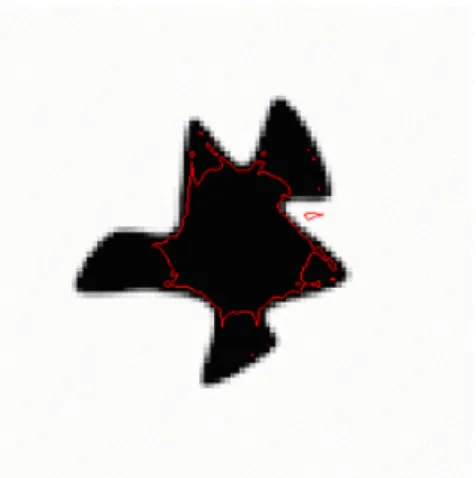
Fig 4.8 Bubble effect

This is the experimental result of level set method using forward differential scheme. The bubble effect refers to the occurrence of unexpected bubbles during the propagation of the curve.

To overcome this phenomenon, the upwind differencing scheme is proposed by [7]. ]) ) 0 , min( ) 0 , [max( ( _, _, , 1 , − + + ₌ ₊_∆ ₋ _∇ ₊ _∇ j i j i n j i n j i u t F F u

where we lower script u and F by their grid indices, u_i_,_j ≡u(i, j)and , and the upper script of u denotes the number of iteration and ) , ( , F i j F_i _j ≡

[

]

[

]

⎪ ⎪ ⎪ ⎪ ⎩ ⎪ ⎪ ⎪ ⎪ ⎨ ⎧ − = − = − = − = + + + = ∇ + + + = ∇ + + − − + + − − − + − + − + − + − + n j i n j i y ij n j i n j i y ij n j i n j i x ij n j i n j i x ij y ij y ij x ij x ij y ij y ij x ij x ij u u D u u D u u D u u D D D D D D D D D , 1 , 1 , , , , 1 , 1 , 2 1 2 2 2 2 2 1 2 2 2 2 , , , , ) 0 , min( ) 0 , max( ) 0 , min( ) 0 , max( , ) 0 , min( ) 0 , max( ) 0 , min( ) 0 , max( In 1D case it is

(33)

]) ) 0 , min( ) 0 , [max( ( 1 + − + ₌ ₊_∆ ₋ _∇ ₊ _∇ i i n i n i u t F F u where

[

]

[

]

⎪ ⎪ ⎩ ⎪ ⎪ ⎨ ⎧ − = − = + = ∇ + = ∇ + + − − − + − + − + n i n i x i n i n i x i x i x i x i x i u u D u u D D D D D 1 1 2 1 2 2 2 1 2 2 , , ) 0 , min( ) 0 , max( , ) 0 , min( ) 0 , max(

The value on each grid of the speed function is greater than zero, those u’s located at troughs will not be updated. Therefore, the grid will not be updated in iteration 3 and remains its value until it is equal to

) (a u

) (a x

u −∆ such that reduces the trend to produce large discontinuities.

Notice that in iteration 2 u(a+∆x) is not a trough and, not like , will be updated in iteration 3 by the upwind differencing scheme. This leads to the fact that

might be updated with a lower value than and will become non-trough at iteration 3 such that is need to be updated in iteration 4. So, it seems that upwind differencing scheme just lower down to touch the x-axis but will eventually becomes a member of the zero level set. However, we will show that this worry is unnecessary under the satisfaction of Courant-Friedriches-Lewy (CFL) condition [7]. That is, is still a trough (

) (a u ) (a x u +∆ u(a) u(a) ) (a u u(a) ) (a u u(a)<u(a+∆x)) at iteration 3 such that it will not be updated at the next iteration if CFL condition is satisfied. Let the discontinuity at iteration 2 be ρ =u(a+∆x)−u(a). Note that ρ > >0. The CFL δ condition is, for each grid point

x t F∆ <∆

And without lost of generality, we can let ∆x=1, therefore F∆t<1. Now we will prove u(a)<u(a+∆x) at iteration 3.

(34)

[

]

[

]

2 2 2 2 1 2 2 2 2 2 2 2 2 2 1 2 2 2 2 3 ) 0 , 1 min( ) 0 , max( 1 0 ) 0 , min( ) 0 , max( ) ( 0 ) ( a x a x a x a x a x a x a x a x x a a x a x x a x x a x x a x a x a x a x a x a u u tF u tF u u u D u u D D D tF u F t u u x a F = − > ∆ − = + ∆ − = = − = > > = − = + ∆ − = ∇ − ∆ + = > ∆ + ∆ + ∆ + ∆ + ∆ + ∆ + ∆ + ∆ + + ∆ + ∆ + − ∆ + + ∆ + − ∆ + ∆ + ∆ + + ∆ + ∆ + ∆ + ρ ρ ρ δ ρ Q

It is easy to derive a general form n by mathematical induction.

a n x a u u + > ∆ +1

(35)

5. Shape Prior

In this chapter, we present how we combine the shape prior with Abdol-Reza’s model. The shape prior refers to knowledge of shape models which we have known that can be used to guide the propagation of the curve. The sections contain geodesic active contour model that is used to represent the shape prior and a distance measure for measuring the dissimilarity between the propagating curve and the shape prior.

5.1. Geodesic Active Contour Model

Let be a binary image with ones on the region R0, after rotated an angle θ

and translated a distance δ, and zeros on the remaining domain. R0 is indeed the

region of the object captured by the curve in the previous frame image In, and the

binary image containing R0 after the transformation is used to construct the

shape prior for the current image In+1_{. During the curve}

1 , , 0 + n R J _θ_δ 1 , , 0 + n R J _θ_δ γ is propagating to capture the object in In+1, the binary image for the shape prior is reconstructed each

time before computing equation (5.1) in each iteration. The region R0 in the binary

image only subjects to a rotation θ and a translation δ to align with the propagating curve 1 , , 0 + n R J _θ_δ

γ , and never deforms its shape all the time (in processing In+1). Although the transformation is limited to rotation and translation in this thesis, it can be extended to combinations of several affine transforms such as scaling and shearing. Now we will define the energy functional

) , , ( ) , , (_γ _I _I 1 _R₀ _E _u _θ _δ E E n n _s r + = r + _(5.1)

(36)

where the image energy Er is equation (4.1) used to perform discriminate analysis on each pixel and the shape energy Es is

∫

⋅ ⋅ = 1 + 0 1 , ( )) ( ) ( , 0 ds ds d J g E w E n R s γ γ δ θ γ r r _(5.2)

where w(Er) is a weighting function ,which means the shape prior is image

energy dependent. For pixels that can clearly classified by Er, the weight is low. If the pixel lies in an uncertainty state, the weight is high and the shape prior will leads the classification. This novelty, different from most existing methods that the weights used to combine the terms of the energy functional are usually constant thresholds, offers more flexibility in the propagation of the contour. In particular, the shape prior will not constrain the deformability of the shape of the object in many cases.

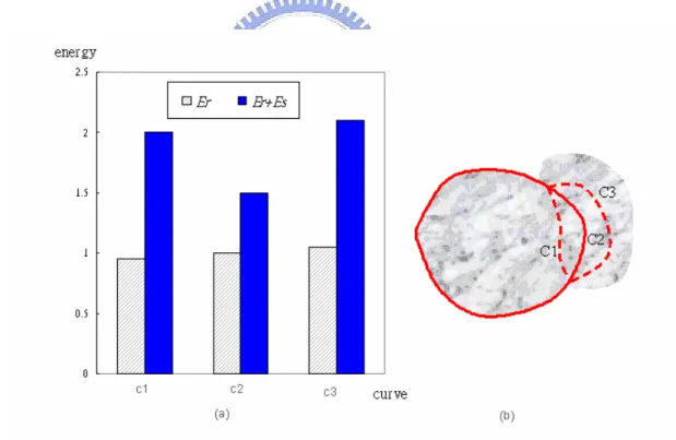
Fig 5.1 Image energy and Shape energy

The energy for the curve c1, c2 and c3 is almost identical, but the energy for c2 is lowered than the others after plus the shape energy.

(37)

the background that is textured with similar appearance to it. Either the curve expands (c3) or shrinks (c1), the energy changes are difficult to distinguish. However, after plus the shape energy, we can eliminate this uncertainty and make a decision.

Despite the weighting function, the term Es comes from the geodesic active contour model. g(I) stands for _p

Iˆ

1 1 ∇

+ , where Iˆ is a smoothed version of I,

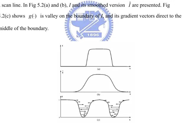
computed using Gaussian filtering, and p = 1 or 2. means that to convert the binary image to an image with continuous numbers from zero to one. Also, if we view the image in 3-dimensional space, the valley will locate at the boundary of the object in the binary image . Fig 5.2 is the observing intensity of a binary image crossed by a scan line. In Fig 5.2(a) and (b), I and its smoothed version

1 , , 0 + n R J _θ_δ

Iˆ are presented. Fig 5.2(c) shows is valley on the boundary of I, and its gradient vectors direct to the middle of the boundary.

) (⋅ g

Fig 5.2 Gradient vector

(a) The intensity signal on a scan line over the binary image. (b) The smoothed version of (a). (c) The derived function g. The evolving contour is attracted to the middle of the boundary by the forces created by∇g⋅∇u.

(38)

The integration (5.2) means the sum of ( 1 ( )) , , 0θδ γ r + n R J

g over the locations occupied by the curveγ multiplied by its piece of length. Since the derived function

takes small values on positions corresponding to the boundary of the object in the binary image, we can expect that the minimum is obtained when the curve is aligned to the boundary of the object in the binary image. To minimize the integration, we search for its gradient descent direction, which is computed from the

Euler-Lagrange equation ) (⋅ g

[

g J g J n

]

n E w t t n R n R r r r r r r −∇ ⋅ = ∂ ∂ ( ) ₍ ₎ ₍ + ₍ ₎₎ ₍ +1 ₍ ₎₎ , 1 , 0, , 0 γ κ γ γ δ θ γ δ θ γ (5.3)

The term∇g attracts the movement of the curve towards the boundary of shape (⋅) prior. An example is given in Fig 5.3. Letw(E_γ)=1 to clarify the effect of the vector field.

Fig 5.3 Shape and its forces field

(a) A binary image J of size 20x20 containing a circle object. (b) The corresponding gradient vectors∇g⋅∇u represent the forces that attract the curve to the pointed direction.

(39)

the level set representation as described in the previous chapter. u u u J g J g E w t u n R u n R ⎥∇ ⎦ ⎤ ⎢ ⎣ ⎡ ∇ ∇ ⋅ ∇ − = ∂ ∂ ₍ ₎ ₍ + ₎ ₍ +1 ₎ , 1 , 0, , 0θδ θδ γ κ (5.4)

Combining (5.4) with (4.4) we can obtain

[

]

u u u x J g x J g E w u x u R I x I P R I x I P t x u n R u n R u n n x out n n x in ∇ ⎥ ⎦ ⎤ ⎢ ⎣ ⎡ ∇ ∇ ⋅ ∇ − + ∇ − ∇ − = ∂ ∂ + + + + )) ( ( )) ( ( ) ( ) ( ) , ) ( ( log ) , ) ( ( log ) ( 1 , 1 , 0 1 , 0 1 , , 0 , 0θδ θδ γ κ λκ (5.5) where β α γ + − = + + ₍ ₎ _, ₎ _log ₍ ₍ ₎ _, ₎ ( log ) ( 0 1 , 0 1 , I x I R P I x I R P E w n n x out n n x in (5.6)

The weighting function is related to the reciprocal of the image energy, where α ( > 0) and β ( > 1) are two user specified constants. When the uncertainty occurs, the weight will take a large value, and, on the other hand, the weight is low when the classification can be confirmed. The purpose of the shape prior is to lead the propagation when the classification is uncertain when the term is almost equal either the contour shrinks or expands.

γ

E

Before computing equation (5.5), however, we need to reduce the involved parameters, that is, to compute θ* and δ* which are the optimizing transform of the shape prior to align with the contour. The final level set equation is (5.7).

[

]

4 4 4 4 4 4 4 4 4 4 3 4 4 4 4 4 4 4 4 4 4 2 1 4 4 4 4 4 4 4 4 4 4 4 4 4 3 4 4 4 4 4 4 4 4 4 4 4 4 4 2 1 r r Es n R u n R E u n n out n n in u u u u J g u J g E w u s u R I x I P R I x I P t x u r ∇ ⎥ ⎦ ⎤ ⎢ ⎣ ⎡ ∇ ∇ ⋅ ∇ − + ∇ − ∇ − = ∂ ∂ + + + + )) ( ( )) ( ( ) ( ) ( ) , ) ( ( log ) , ) ( ( log ) ( 1 * *, 1 * *, 0 1 , 0 1 , , 0 , 0θ δ θ δ γ γ γ κ κ λ (5.7)

(40)

This is done by using a dissimilarity measurement between distance functions of the curve and the shape prior. We will discuss this subject in the next section.

5.2. An Euclidean Invariant Shape

Prior

Computing θ* and δ* separately eliminates translation and rotation from the shape energy Es and no additional parameters entering the minimization. A commonly alternative approach is to explicitly model a translation and an angle and minimize with respect to these quantities (by gradient descent or other). In Daniel Cremers et al.’s opinion [20], the explicitly model has several drawbacks:

1. The introduction of explicit pose parameters makes numerical minimization more complicated— corresponding parameters to balance the gradient descent must be chosen. In practice, this is not only tedious, but it may cause numerical instabilities if the corresponding step sizes are chosen too large.

2. The joint minimization of pose and shape parameters mixes the degrees of freedom corresponding to translation and rotation with those corresponding to shape deformation.

3. Potential local minima may be introduced by the additional pose parameters. In a given application, this may prevent the convergence of the contour towards the desired segmentation.

Therefore, to reduce the parameters in minimizing Es, we compute θ* and δ* and reconstruct the binary image before computing (5.7). The idea of evolution process thus consists of two phases:

1. Aligning the shape prior with the curve (compute θ* and δ*).

(41)

Phase 1: Minimize Es (Equation 5.10)

Each iteration of the algorithm consists of the following steps:

Step 0. Manually draw the initial contour of the object being tracked in the first frame such that the contour points contain the desired object boundary. You may exclude the shadow. Set the current frame number to 2.

Step 1. Use the contour obtained in the previous frame as the initial contour and the prior shape of the current frame.

Step 2. Compute the rotation and translation parameters between the current contour and the prior shape (see equation 5.10)

Step 3. Do for all contour points one at a time:

use equation 5.7 to compute Er, Es, and W(Er). Then update the level set value

at the contour point.

Phase 2: Minimize Er+Es (Equation 5.7) Stop? Stop? N N Y Y

(42)

Step 4. After all the contour points are updated, check if the contour does not

converge or the number of iteration does not exceeds a specified upper bound; if not, go to Step 2; otherwise, terminate with the contour as the final contour of the current frame.

Step 5. Is the frame the final frame? If yes, stop; otherwise, increase the frame number by 1 and go to Step 1.

The evolution process is performed iteratively to minimize the energy functional (6). The idea is illustrated in Fig 5.4 and Fig 5.5.

Fig 5.4 Shape prior illustration 1

Fig 5.4 presents that the contour (the red curve) will neglect the shape prior (the blue equal signs curve) to capture the object (the rectangle) when it can distinguish the object from the background (the circle). In Fig 5.4(a), a rectangular object staying at the bottom is textured with marble appearance, and at the top locates a part of the background that is also textured with marbles. A red curve is initialized to properly capture the object. Then, the object moves upwards with a small distance in Fig 5.4 (b). The evolution process of the curve is shown in Fig 5.4(c) and Fig 5.4(d). Fig 5.4(c) is the early phase of the computation, that is, to align the shape prior with the curve.

(43)

the shape can completely align with the curve. In Fig 5.4(d), the computation enters the 2nd phase and the curve starts to move according to the image information and the attraction of the shape prior. However, because the curve can distinguish the object from the background, which is white at this time, the curve just moves to capture the object directly, ignoring the shape prior.

Fig 5.5.Shape prior illustration 2

The object continuously moves upwards and, at this time, overlaps with the part of the background that is similar to the object.

Fig 5.5 presents the idea of the shape prior to capture the object involved in the background in this figure. Fig 5.5(a) is the capturing result of Fig 5.4 and also the initialization of Fig 5.5, with the curve properly captured the object. Then the object moves with a large step into the background in Fig 5.5(b). Now, the remaining figures are trying to capture the object. Fig 5.5(c) is to align the shape prior with the curve. As

(44)

in Fig 5.4(c), it is completely matched with the contour. However, in Fig 5.5(d), the attraction of the shape prior takes effect. The bottom part of the curve, again, moves freely to capture the bottom of the object since the curve knows where the object is, but the top part of the curve is locked by the shape prior because it dose not known the marbles above belongs to the object or belongs to the background. This is because the marble at the bottom can only belongs to the object since no similar background is around it, and the marble at the top has alternative choices. Continuously, the shape prior is aligned with the curve in Fig 5.5(e). However, the size of the curve has changed. To make the alignment possible, the best solution is to place the curve in the center of the shape prior, as shown in the figure. After this arrangement, the curve can continuously evolve in Fig 5.5(f). But opposed to Fig 5.5(d), the bottom part of the curve stays at the same location but the top part can take liberty to move upwards by the attraction of the shape prior. Note that the top part of the curve is moving towards the actual boundary of the object by the leading of the shape prior after its alignment, and the certain parts of the curve can stay at its positions. In Fig 5.5(g) and Fig 5.4(h), the evolving process repeats continuously in this way. The shape prior goes upwards with a little step in Fig 5.4(g), and then the top part of the curve is attracted upwards. After several iterations, the curve can capture the object with an allowable error.

Now we formulate the computation of θ* and δ* now. A dissimilarity measure is calculated for two distance functions. Let R₀(θ,δ)denotes the region after rotated an angle θ and translated a distance δ. Let φ0 be the distance function of∂R0(θ,δ), the

boundary ofR₀(θ,δ), over the domain Ω. Let φ1 be the distance function of the

propagating curve (the level set u = 0) overΩ. The dissimilarity measure between φ0

(45)

dx h h x x x x d

∫

Ω + − = 2 ) ( ) ( )) ( ) , , ( ( )) ( ), , , ( ( 2 0 1 1 0 1 0 2 _φ _θ _δ _φ _φ _θ _δ _φ φ φ _(5.8) = f(θ,δ)= f(ρ) where

∫

Ω

=

⎩

⎨

⎧

≥

=

dx

H

h

else

0 H

)

(

)

(

)

(

,

0 ,

1 )

(

φ

This distance measure is symmetric but merely a pseudo-distance [22]. The minima of (5.8) occurs at 2( 0, 1) ₌0 ∂ ∂ ρ φ φ d

. Let ρ ={θ,δ} be the pose parameters, the optimization ρ*={θ*,δ*}can be derived by calculating the gradient descent direction ρ ∂ ⋅ ∂ − d2() and is given by

[

]

dx H dx h h t ρ φ φ δ φ φ φ φ φ ρ φ φ φ φ φ ρ ∂ ∂ − − − − ∂ ∂ + − − = ∂ ∂

∫

Ω Ω Ω 0 0 2 0 1 2 0 1 0 0 1 0 1 ) ( ) ( ) ( ) ( 2 1 )) ( ) ( ( ) ( (5.9)

where )δ_ε(s)=H_ε′(s is delta function, which is chosen to have and infinite support: 2 2 1 ) ( s s + = ε ε π δ_ε and

∫

− = − ) ( ) h( )dx ( 2 ₀ 0 1 2 0 1 φ φ φ φ φ

Notice that the distance measure (5.8) is not an energy functional and (5.9) is derived by computing its gradient descent direction but not derived from computing

(46)

Euler-Lagrange equation. Then, equation (5.9) can be used to solve the optimal pose parameters θ* and δ* iteratively.

(47)

Proof of (5.9):

[

]

[

]

value. very small a or t Let dx H dx h h dx dx h H dx h h dx dx h H dx h h dx dx h H dx h h dx dx h H dx h h dx dx H dx h dx H dx h h dx dx H dx H dx H dx h h dx dx H H dx h h dx h dx h h h dx h h dx h h d t 0 ) ( ) ( ) ( ) ( 2 1 )) ( ) ( ( ) ( ) ( ) ( ) ( ) ( ) ( 2 1 )) ( ) ( ( ) ( ) ( ) ( ) ( ) ( ) ( ) ( 2 1 )) ( ) ( ( ) ( ) ( ) ( ) ( ) ( ) ( ) ( 2 1 )) ( ) ( ( ) ( ) ( ) ( ) ( ) ( ) ( 2 1 )) ( ) ( ( ) ( ) ( ) ( ) ( ) ( ) ( ) ( 2 1 )) ( ) ( ( ) ( ) ) ( ( ) ( ) ( ) ( ) ( ) ( 2 1 )) ( ) ( ( ) ( ) ( ) ( ) ( 2 1 )) ( ) ( ( ) ( ) ( ) ( 2 1 )) ( ) ( ( ) ( ) ( 2 ) ( )) ( ) ( ( ) ( 2 ) ( ) ( ) ( 0 0 2 0 1 2 0 1 0 0 1 0 1 0 0 0 2 0 1 2 0 1 0 0 0 1 0 1 0 2 0 1 0 0 0 0 2 0 1 0 0 0 1 0 1 0 0 0 2 0 1 0 0 2 0 1 0 0 0 1 0 1 0 0 0 0 0 2 0 1 0 0 0 1 0 1 0 0 0 0 0 0 0 2 0 1 0 0 1 0 1 2 0 0 0 0 0 0 0 2 0 1 0 0 1 0 1 0 0 2 0 1 0 0 1 0 1 0 2 0 1 0 0 1 0 1 0 2 0 1 0 0 1 0 1 0 1 2 0 1 2 → ∂ ∂ ∂ ∂ − − − − ∂ ∂ + − − = ∂ ∂ − − − − ∂ ∂ + − − = ⎥ ⎦ ⎤ ⎢ ⎣ ⎡ − ∂ ∂ − ∂ ∂ − − ∂ ∂ + − − = ⎥ ⎦ ⎤ ⎢ ⎣ ⎡ ∂ ∂ − − ∂ ∂ − − ∂ ∂ + − − = ⎥ ⎦ ⎤ ⎢ ⎣ ⎡ ∂ ∂ − ∂ ∂ − − ∂ ∂ + − − = ⎥ ⎥ ⎥ ⎥ ⎦ ⎤ ⎢ ⎢ ⎢ ⎢ ⎣ ⎡ ∂ ∂ − ∂ ∂ − − ∂ ∂ + − − = ⎥ ⎥ ⎥ ⎥ ⎦ ⎤ ⎢ ⎢ ⎢ ⎢ ⎣ ⎡ ∂ ∂ − ∂ ∂ − − ∂ ∂ + − − = ∂ ∂ − − ∂ ∂ + − − = ∂ ∂ − − ∂ ∂ + − − = ∂ ∂ − + ∂ ∂ + − − = ⎥⎦ ⎤ ⎢⎣ ⎡ ₋ + ∂ ∂ − = ∂ ∂ − = ∂ ∂

∫

_∫

∫

_∫

∫

Ω Ω Ω Ω Ω Ω Ω Ω Ω Ω Ω Ω ρ ρ φ φ δ φ φ φ φ φ ρ φ φ φ φ φ ρ φ φ δ φ φ φ φ φ φ ρ φ φ φ φ φ φ φ φ ρ φ φ δ ρ φ φ δ φ φ φ ρ φ φ φ φ φ ρ φ φ δ φ φ φ ρ φ φ δ φ φ φ ρ φ φ φ φ φ ρ φ φ δ φ ρ φ φ δ φ φ φ ρ φ φ φ φ φ φ ρ φ φ δ φ φ ρ φ φ δ φ φ ρ φ φ φ φ φ φ ρ φ φ δ φ φ ρ φ φ δ φ φ ρ φ φ φ φ φ φ φ ρ φ φ ρ φ φ φ φ φ ρ φ φ φ ρ φ φ φ φ φ ρ φ φ φ ρ φ φ φ φ φ φ φ φ φ ρ ρ ρ ε ρ ρ ρ ρ ρ ρ ρ ρ < ∂ ∂ − = ∂ ∂ − ⋅ + = = = + k k d until repeat h d h k k | ; 1 . 0 ; | 2 2 1

(48)

6. Experiments

There are three experiments. Experiment 1 explores the characteristics of the tracking method. Experiment 2 presents the mechanism of the shape prior. Finally we use real image sequences in experiment 3.

6.1. Synthetic Image Sequences

This experiment is to explore characteristics of the tracking method.

(a) Small Displacement

There are three cases in this experiment. Case 1 is an object with homogeneous color moving from left to right and approaching a background texture that is similar to the object. In case 2, an object with a small part of it is pasted by the background texture. The object is moving from left to right in a homogeneous background. Finally in case 3 is a combination of case 1 and case 2. An object with a small part similar to the background is moving approaching a background texture that is similar to that object. The image sequence is of size 80x100 each. Since the move takes 6 pixels, we set the size of the searching window η = 7. Number of iterations = 40.

Both two methods can capture the object correctly. In figure 3 and figure 4, the nearest distance between the background-like texture within the object and its boundary is 14 pixels. In figure 5 and figure 6, the least distance between the object and the object-like background is 8 pixels. The size of searching window is 7 pixels. Therefore, each pixel is under certainty and we can get good results.

(49)

Fig 6.1 Abdol-Reza’s model

(50)

(51)

Fig 6.6 Abdol-Reza’s model + Shape prior

(b) Large Displacement

This experiment is similar to experiment 1, but with a large move distance. We take frame 1, 3, 6 from each case in experiment 1 and compare the two approaches. The move distance is 18 pixels. We set the size of searching window η = 20 and the number of iterations is 80.

(52)

Abdol-Reza’s model’s model failed. In frame 2 of figure 1, the distance between the pixels around the corrupted contour and the background-like part in frame 1 is at most 14 pixels. However, since the search range is 20 pixels, we cannot determine the pixels left to the object as the object or background.

In figure, since the right part of the contour can correctly capture the object, it drags the shape to right and make the alignment. Then the left part of the contour is compensated by the shape prior and we can get the good result.

Similarly, in figure 4 the right part of the contour is determined by shape prior which is pushed by the left of the contour.

In figure 5 and figure 6, both methods failed. The right and left part of the contour cannot certainly to align the shape, thus the shape cannot be attracted to right position. This case can be handled by background registration and removal before contour propagation. The result is in figure 7.

(53)

Fig 6.9 Abdol-Reza’s model.

Fig 6.10 Abdol-Reza’s model + Shape prior.

Fig 6.11 Abdol-Reza’s model.

(54)

(55)

6.2. Digital Camera Photos

This experiment presents an image sequence that is composed of digital photos that are captured by a digital camera. The object is manually outlined in frame (a) then transforms gradually in later frames. We will present how the shape prior works when the object is partially involved in the background. We have set η = 10 pixels, and the number of iteration is 80.

Fig 6.14 presents Abdol-Reza’s model. In frame (b), when the object rotates a small angle, its bottom-right corner is near a similar background and the contour shrinks there. The shrinking continues in frame (c) and frame (d). Finally in frame (e), after the object moves away from the similar background, the contour cannot recover since some part of the object is regarded as background in frame (d) and that part will result in misclassification in the next frame.

(56)

Fig 6.15 illustrates our approach. In frame (b) the bottom-right corner of the contour is prevented from shrinking by the shape prior. In frame (c), the left part of the object is certain and can used to align the shape correctly. After the shape

alignment, the involved part of the object can be preserved by the shape. As the same reason, the object can be captured correctly in the later frames. We will present how the shape works in the next figure.

Fig 6.15. Abdol-Reza’s model + shape prior on digital camera photos

Fig 6.16 shows how the shape prior works. Figure (a) is previous frame and figure (b) from figure (i) are current frames (To clarify that Fig 6.16 is not an image sequence but the process during contour propagation, we use the term figure (.) or simply (.) instead of frame (.). ) The red curve is the propagating contour and the blue curve is the shape prior. The contour and the shape prior are initialized as the result of the previous frame (which is manually outlined in (a) in this illustration). Then the object rotates clockwise with an angle. In (b)(c), the left part of the contour is far from the similar background, which will be excluded by the searching window, is under

利用等位函數法結合形狀資訊做影像序列的物體追踪

國立交通大學

資訊工程學系

碩士論文