基於H.264/AVC的混合式多重描述編碼

全文

(1)國立交通大學資訊科學與工程研究所碩士論文. 基於 H.264/AVC 的混合式多重描述編碼. Hybrid Multiple Description Coding Based on H.264/AVC. 研究生：蕭家偉指導教授：蔡文錦. 中華民國. 教授. 九十七. 年七月.

(2) 基於 H.264/AVC 的混合式多重描述編碼 Hybrid Multiple Description Coding Based on H.264/AVC. 研究生：蕭家偉. Student：Chia-Wei Hsiao. 指導教授：蔡文錦. Advisor：Wen-Jiin Tsai. 國立交通大學資訊科學與工程研究所碩士論文. A Thesis Submitted to Institute of Computer Science and Engineering College of Computer Science National Chiao Tung University in partial Fulfillment of the Requirements for the Degree of Master in Computer Science July 2008 Hsinchu, Taiwan, Republic of China. 中華民國九十七年七月. ii.

(3) 基於 H.264/AVC 的多重描述編碼學生 : 蕭家偉. 指導教授 : 蔡文錦教授國立交通大學資訊科學與工程研究所. 摘. 要. 在即時視訊傳輸系統，如視訊會議、點對點視訊串流或是網路電視，時常會有網路連線瞬間中斷導致的視訊品質低落，甚至無法解碼的情形。當錯誤發生時，如果等待重新傳送先前發生錯誤的封包則會使得接收端的播放延誤。多重描述編碼是一個相當適合解決此種問題的系統架構。其特性是不使用重傳機制而將原始資訊平均分散在多個描述子，任一個描述子都可單獨解碼還原，接收的描述子越多則還原的品質越佳。此篇論文中，我們提出一個基於 H.264/AVC，在空間域與頻率域中切割資訊的多重描述編碼架構模型，包含編碼端與解碼端。在編碼端中，對任一個原始視訊，在編碼過程中，會經由空間域的第一次切割產生兩個描述子，接著於頻率域進行第二次切割產生四個描述子。而在解碼端會在解碼過程中將所接收到的描述子合併。當有描述子發生錯誤或遺失時，在解碼時會利用空間域與頻率域上的相關性來達成錯誤隱藏，以增進視訊的品質。由實驗結果可得到，相較於先前之基於空間域方法，在發生描述子錯誤時，可以有較好的表現. 關鍵字 : 多重描述編碼、多相重排與次取樣、誤配控制、錯誤隱藏 iii.

(4) Hybrid Multiple Description Coding Based on H.264/AVC Student: Chia-Wei Hsiao. Advisor: Dr. Wen-Jiin Tsai. College of Computer Science National Chiao Tung University. Abstract In real-time video streaming systems, such as, video conferencing, peer-to-peer video streaming or IPTV, network errors frequently occur and result in degradation of video quality or failure to decode the bit-stream at the receiver. Retransmission of error packets imposes unacceptable delay of the video sequence. Multiple description coding (MDC) is an ideal approach, which generates multiple descriptors with equal importance, to overcome such problem. In this thesis, a H.264/AVC based multiple description coding model, which splits information in spatial and frequency domain, is proposed. In the encoder, two descriptors will be generated after the first splitting in the spatial domain, and then the second splitting is done in the frequency domain for each descriptor, resulting in four descriptors in total. In the case of descriptor loss, the decoder will utilize the correlations in spatial domain and frequency domain for error concealment. The experimental results show that the proposed hybrid model has better RD performance than the existing spatial domain based MDC model.. Keywords: Multiple description coding, Polyphase permutation and sub-sampling, Mismatch control, Error concealment iv.

(5) Table of Contents CHAPTER 1.. INTRODUCTION .................................................................................................. 1. 1.1. PREFACE................................................................................................................................ 1. 1.2. MULTIPLE DESCRIPTION CODING........................................................................................ 4. CHAPTER 2. RELATED WORK .................................................................................................... 7 2.1. CLASS A MDC MODEL ......................................................................................................... 7. 2.2. CLASS B MDC MODEL ......................................................................................................... 9. CHAPTER 3. MOTIVATION ........................................................................................................ 13 CHAPTER 4. D4 AND R4 MODELS ............................................................................................. 15 4.1. DUPLICATED INFORMATION ............................................................................................... 15. 4.2. D4 MODEL .......................................................................................................................... 16. 4.2.1. D4 Encoder .................................................................................................................... 16. 4.2.2. Error Concealment in D4 .............................................................................................. 19. 4.3. R4 MODEL .......................................................................................................................... 21. 4.3.1. R4 Encoder .................................................................................................................... 21. 4.3.2. Error Concealment in R4 .............................................................................................. 23. CHAPTER 5. HYBRID MODEL ................................................................................................... 25 5.1. HYBRID ENCODER .............................................................................................................. 25. 5.1.1. Polyphase Permuting and Splitting ............................................................................... 26. 5.1.2. Coeff Splitter .................................................................................................................. 28. 5.1.3. Frequency and Spatial Merge ....................................................................................... 32. 5.2. HYBRID DECODER .............................................................................................................. 33. 5.2.1. Spatial Concealment ...................................................................................................... 35. 5.2.2. Frequency Concealment ................................................................................................ 37. CHAPTER 6. EXPERIMENTAL RESULTS ................................................................................. 41 6.1. THREE DESCRIPTORS ......................................................................................................... 42. 6.2. TWO DESCRIPTORS............................................................................................................. 46. 6.3. ONE DESCRIPTOR ............................................................................................................... 50. 6.4. PACKET LOSS SIMULATION ................................................................................................ 54. CHAPTER 7. CONCLUSION........................................................................................................ 56 REFERENCE ................................................................................................................................. 57. v.

(6) List of Figures FIGURE 1.1 CONVENTIONAL MDC SYSTEM ARCHITECTURE .............................................................. 4 FIGURE 2.1 ENCODER SYSTEM ARCHITECTURE OF [6]. FROM [6]. ..................................................... 8 FIGURE 2.2 INDEX ASSIGNMENT OF SCALAR QUANTIZER. FROM [6].................................................. 8 FIGURE 2.3 PSS SYSTEM ARCHITECTURE .......................................................................................... 11 FIGURE 2.4 POLYPHASE SUB-SAMPLING............................................................................................. 11 FIGURE 2.5 PATTERN FOR RECEIVING THREE DESCRIPTORS ........................................................... 12 FIGURE 4.1 ENCODER ARCHITECTURE OF D4 MODEL. ..................................................................... 16 FIGURE 4.2 4X4 BLOCK PROCESSING ORDER IN A MACROBLOCK .................................................... 17 FIGURE 4.3 AC COEFFICIENT ASSIGNMENT IN A 4X4 BLOCK............................................................ 18 FIGURE 4.4 FOUR 4X4 BLOCK TYPES THE ROTATING SPLITTER GENERATES .................................. 19 FIGURE 4.5 4X4 BLOCK TYPE DISTRIBUTION IN A MACROBLOCK .................................................... 19 FIGURE 4.6 4X4 BLOCK COEFFICIENT PREDICTION DIRECTION ...................................................... 20 FIGURE 4.7 COEFFICIENT PREDICTION AND DESCRIPTOR 3 IS LOST ................................................ 21 FIGURE 4.8 ENCODER ARCHITECTURE OF R4 MODEL ...................................................................... 22 FIGURE 4.9 RES SPLITTER SPLITS ONE MACROBLOCK INTO FOUR ONES ........................................ 22 FIGURE 4.10 AN MACROBLOCK PATTERN AFTER LOSS DESCRIPTOR 3 ........................................... 23 FIGURE 5.1 HYBRID ENCODER ARCHITECTURE ................................................................................ 25 FIGURE 5.2 POLYPHASE PERMUTING OF A 8X8 BLOCK ...................................................................... 27 FIGURE 5.3 SPLITTING OF A 8X8 BLOCK............................................................................................. 28 FIGURE 5.4 GROUPS OF FREQUENCY IN 4X4 BLOCK.......................................................................... 29 FIGURE 5.5 EVEN AND ODD 4X4 BLOCKS ARE GENERATED BY COEFF SPLITTER ............................ 30 FIGURE 5.6 MACROBLOCK PATTERN AFTER TWO LEVEL SPLITTING .............................................. 31 FIGURE 5.7 THE COEFF MERGER IN FREQUENCY DOMAIN .............................................................. 32 FIGURE 5.8 THE RESIDUAL MERGING AND POLYPHASE INVERSE PERMUTATION ............................ 33 FIGURE 5.9 HYBRID DECODER ARCHITECTURE ................................................................................ 34 FIGURE 5.10 SPATIAL CONCEALMENT FOR ONE RECEIVED DESCRIPTOR ........................................ 35 FIGURE 5.11 SPATIAL CONCEALMENT FOR TWO RECEIVED DESCRIPTORS ..................................... 36 FIGURE 5.12 SPATIAL CONCEALMENT BY BILINEAR INTERPOLATION .............................................. 36 FIGURE 5.13 AC PREDICTION FOR TWO RECEIVED DESCRIPTORS .................................................. 38 FIGURE 5.14 AC PREDICTION FOR THREE RECEIVED DESCRIPTORS ............................................... 38 FIGURE 5.15 RESULTS OF QUALITIES BY VARYING NUMBER OF CONCEALED ACS .......................... 39 FIGURE 6.1 PSNR OF THREE RECEIVED DESCRIPTORS AT DIFFERENT BIT-RATES.......................... 43 FIGURE 6.2 PSNR OF EACH FRAME OF RECEIVING THREE DESCRIPTORS. ..................................... 45 FIGURE 6.3 PSNR OF TWO RECEIVED DESCRIPTORS AT DIFFERENT BIT-RATES. ............................ 47 vi.

(7) FIGURE 6.4 PSNR OF EACH FRAME OF RECEIVING TWO DESCRIPTORS. ........................................ 49 FIGURE 6.5 PSNR OF ONE RECEIVED DESCRIPTORS AT DIFFERENT BIT-RATES. ............................. 51 FIGURE 6.6 PSNR OF EACH FRAME OF RECEIVING ONE DESCRIPTOR. ........................................... 53 FIGURE 6.7 PSNR DEGRADATION OF PACKET LOST IN DESCRIPTORS ............................................. 55. vii.

(8) List of Tables TABLE 1.1 BENEFITS OF ERROR RESILIENCE TOOLS ACCORDING TO CATEGORY. FROM [1]............... 2 TABLE 5.1 SUMMARY OF SPATIAL AND FREQUENCY CONCEALMENT CASES .................................... 34 TABLE 6.1 QUALITY OF EACH MODEL AT 100 KBIT/S PER DESCRIPTOR........................................... 46 TABLE 6.2 QUALITY OF EACH MODEL AT 100 KBIT/S. ....................................................................... 50 TABLE 6.3 QUALITY OF EACH MODEL AT 100 KBIT/S. ....................................................................... 54. viii.

(9) Chapter 1 Introduction. 1.1 Preface Through the growing of the communication technology, video streaming has recently become a popular field. There had been more and more application services about video streaming being developed and provided, such as, IPTV, peer-to-peer (P2P) live video and video phone; the scale of these services also becomes larger. Transmitting video streams smoothly to effectively combat network errors is an important subject. H.264/AVC is one of the most newly introduced video coding standard developed by Joint Video Team founded by ITU-T and ISO/IEC, which has a better video quality and compression efficiency than existing standards, such as MPEG2 and H.263. When transmitting the H.264/AVC encoded bit-stream, as the coding efficiency is higher, the bits of the encoded stream carry more information of the video source, and the bit-stream would be more vulnerable to transmission errors. As a result, there had been a lot of error resilience tools proposed to combat transmitting error; table 1.1 from [1] by A. Vetro, J. Xin and H. Sun summarizes recently proposed error resilience tool. These tools are classified into four different groups according to field of categories and their benefits are listed separately. Localization is a technique that can restrain the error to propagate in a limit range; data partitioning separates the 1.

(10) encoded bit-stream into different parts, each has unequal importance so that one can protect each part with different levels of security; redundant coding protects the bit-stream with additional data bits, that is when error occurs, the correctly received parts can be used to recover the lost parts; concealment-driven aims to predict lost part of data with the aid of correlation on either spatial or temporal domain. H.264/AVC had incorporated almost all tools in the four categories from table 1.1: 1) adaptive intra refresh; 2) reference picture selection; 3) multiple reference pictures; 4) data partition of MV, header and texture; 5) Redundant slice; 6) Flexible macroblock order.. Table 1.1. Benefits of error resilience tools according to category. From [1]. Low-bandwidth handheld devices have become more popular and backbone capacities of the Internet has increased, thus for a video streaming service, the client bandwidth varies in a wide range, from hundreds of kilo-bytes to tens of mega-bytes. Clients on hand-held devices such as cell phone, smart phone or PDA, usually have lower bandwidth, while in desktop, higher bandwidth is common. As a result, a service that is adaptive to the varying bandwidth of heterogeneous networks would 2.

(11) become more appealing. Real-time is another important characteristic in video streaming services. A system that utilizes retransmission or feedback channel may result in an unacceptable delay; since retransmitting lost packets would add at least one round-trip time delay, thus the packet would expired its display timeline. In the streaming on P2P network, the receiving of data stream may come from different source peers through different paths, and the path may failed if one peer along the path failed, thus the receiver could constantly losing part of data from some peers. As the failure of peer is not predictable, the part of data which will get lost during transmission is not know a priori. In this circumstance, using unequal error protection would not be effective. If receivers can make use of whatever they received and utilize the appropriate error concealment and/or resilience tools, the system will have a better performance. Thus, to successfully transmit video stream in heterogeneous error prone networks, we expect that the video streaming system should at least have the following requirements: 1.. Scalable bandwidth and quality . The receivers can be classified into groups by the capability of its bandwidth and display quality; the higher bandwidth, the better quality.. 2.. Equal protection on each part of data . To simplify the transmitting mechanism, each part of data is treated equally.. 3.. Avoiding feedback channel and retransmission . Waiting for the feedback and retransmit the lost packet could imposes a unacceptable delay while playing video. 4.. Error resilience function 3.

(12) . Rising the PSNR when error occurs. Multiple description coding (MDC), in the “Redundant coding” category in table 1.1, is a technique that meet the above criterions.. 1.2 Multiple Description Coding MDC is a technique that encodes a single information source into two or more output streams, called descriptors, and each descriptor can be decoded independently and has an acceptable decoding quality; in addition, the decoding quality will be better if more descriptors were received. Contrary to MDC, single description coding (SDC) is used to indicate the standard encoded bit-stream with H.264/AVC. MDC is first originated from an interesting problem from information theory: If an information source is described with two separate descriptions, what are the concurrent limitations on qualities of these descriptions taken separately and jointly? [2]. This problem was first presented by Wyner and latter became the MD problem. Latter in 1993, Vaishampayan had proposed the first practical implementation of MD, called multiple description scalar quantizer(MDSQ) [4], which proposes two index assignment table: nested index assignment and linear index assignment, that map a quantized coefficient into two indices each could be coded with fewer bits. Afterwards, researches on different implementations of MDC had been proposed, and will be introduced later.. Figure 1.1. Conventional MDC System Architecture 4.

(13) Most MDC approaches focus on how to generate two descriptors so that each descriptor would have good decoding quality and the overall two channel bit-rate would be minimized. Figure 1.1 shows the conventional MDC system architecture. The encoder encodes the source into two individual descriptors and then sends through two channels. The decoder has multiple decoder states: side decoder and center decoder; when receiving only one descriptor, the side decoder will be responsible to decode the one descriptor bit-stream; if both descriptors were received the center decoder will produce the best quality output. Layered coding, such as scalable video coding(SVC), is a technique that encodes the bit-stream into base layer and enhancement layers; base layer has lower bit-rate and a basic acceptable quality of video, and enhancement layers are used to refine the video quality. If the network traffic is congested, the receiver can receive only base layer; if the bandwidth is sufficient for the receiver to obtain more data, the enhancement layers will be used to further refine the decoding quality. The more enhancement layers are received, the better the decoding quality can be obtained. SVC seems to meet the four requirements mentioned in section 1.1 and has similar features with MDC, but they are different in the view of data importance: SVC treats base layer more important, while the descriptors are equally important in MDC. The different importance of base layer and enhancement layers are due to the fact that enhancement layers cannot be reconstructed without the base layer. In other words, if the base-layer data packets are corrupted, then the corresponding enhancement layers‟ data packets will be useless. Contrary to SVC, each descriptor of MDC has equal importance, bit-rate and quality. Consider the case that the information source are encoded into n descriptors in MDC architecture, while in SVC, n-1 enhancement layers and one base layer are generated. In both systems the resulting bit-streams are sent through n separate channels and each channel has average error probability p. 5.

(14) Then, the probability that the receiver can reconstruct the video is: 1) 1-p, for SVC; 2) 1-pn, for MDC. In conventional error prone environment, for example, wireless network, the average error rate p might be 20%, and let n = 2, then the probability to successfully reconstruct the video for MDC is 0.96 (1-0.04), which is higher than 0.8 (1-0.2) for SVC.. 6.

(15) Chapter 2 Related Work. There have been a lot of MDC models proposed since the first implementation, MDSQ [4]. These models can be intuitively classified through the stage where it split the original signal, such as, spatial domain, frequency domain and temporal domain. To be more precisely, in [3], Wang had come up with another classification approach, that is based on the type of predictor a MDC model had adopted and three classes have been defined. Class A focuses on the prediction efficiency; class B focuses on the mismatch control; and Class C controls trade-off between the two issues. Since the performance evaluation of the proposed model will be compared to the models from class A and B, the following sections describe the two models in details.. 2.1 Class A MDC Model MDC models of Class A have the property that the predictor used in the encoder is in accordance with that used in SDC, which has the best prediction efficiency, in other words, the prediction of class A encoder is the same as the center decoder. In motion estimation, the reconstructed reference frames is fully reconstructed in the encoder as if all descriptors are received in the decoder, thus the predictor can find the most similar regions in the reference frames. As a result, the prediction efficiency is efficient using class A. 7.

(16) The first implementation of MDC, MDSQ [4], focuses on splitting general signal source, and latter in [6] had applied the MDSQ approach to H.264/AVC. Figure 2.1 shows the encoder architecture proposed in [6]. It can be observed that it is a typical class A architecture because there is only one prediction loop, and after quantization, the coefficients are split to two paths, generating two descriptors, NAL 1 & NAL 2.. Figure 2.1. Encoder System Architecture of [6]. From [6].. The function of MDSQ block in Figure 2.1 is illustrated in Figure 2.2, where the numbers in the 2D array are quantized DCT coefficients, and each one is mapped to two indexes in vertical and horizontal directions.. Figure 2.2. Index Assignment of Scalar Quantizer. From [6]. 8.

(17) There are a number of class A models based on splitting either frequency coefficients or residual data. In [8], the transformed coefficients are split to two descriptors such that the total distortion and bit-rate of two descriptors are minimized by Lagrange multiplier λ. Even though the generated descriptors have optimal total distortion, the reconstruction quality and bit-rate of descriptors are different, resulting in unbalanced descriptors. In [9], a balanced splitting of coefficients is proposed to combat this issue, in which the splitting process is divided to two stages. First, the coefficients are assigned to two descriptors so that the difference of energy between two descriptors are minimized, which resulting in balanced distortion. Then, the coefficients are swapped to make sure the two descriptors have a nearly the same bit-rate. [10] is another MDC model of class A. It is more flexible in that two or three descriptors can be generated and is also based on frequency coefficients splitting. In [11], the splitting is based on prediction error. The residual of each macroblock after motion compensation is polyphase permuted and the split to two descriptors. Then, a new data partition mode is added to generate two descriptors. 2.2 Class B MDC Model The main characteristic of class B models is prediction mismatch control, which is achieved by taking the state of decoder into account. The prediction in the encoder of class B is the same as that in the side decoder of each descriptor, in other words, it can be viewed as encoding the descriptors separately so that when decoding any one descriptor, the prediction for every macroblock is the same as that in encoder, resulting in better quality compared with class A model in case of descriptor loss. Using class A model, the worse reconstructed quality is due to the loss of partial information used for prediction in the decoder. Thus, the main difference between 9.

(18) class A and class B models is that what information is used for prediction. In class B, the information used for prediction falls into two types: one uses partial information contained in each descriptor for prediction; the other uses the information common in every descriptor for prediction. However, both of these two types result in prediction inefficiency: incomplete information is used for prediction, so that the predicted blocks used may not be the same as those in SDC, resulting in a larger prediction error. Hence, the bit-rate increased for a given quality. A variety of MDC approaches adopt class B model, from simple to complex architectures. The simplest approach might be the one that splits the video sequence to odd and even frames, separately encodes the two groups to form two descriptors and applies error concealment in the side decoders [12]. The prediction inefficiency is increased when the temporal distance is increased. Therefore, if three or more descriptors are to be generated, the prediction for each descriptor becomes more inefficient. In [13], a more complex architecture is proposed. Two type of frames, H-SNR for high quality and L-SNR for low quality, are alternative placed in two descriptors, and two-stage quantization is used. H-SNR frames are produced in the 1st stage and L-SNR frames are produced in the 2nd stage quantization. The mismatch control is done by using the L-SNR frames as reference frames, since H-SNR could be transformed to L-SNR for the 2nd stage quantization in the decoder. This model is an example of class B with the type that uses information common in both descriptors for prediction. [14] is another class B model based on H.264/AVC. It utilizes the slice group with disperse mode which groups macroblocks in a frame to two slices and forms a check board pattern. In one descriptor, one of the two slices is quantized by a higher quantization parameter (QP) and the other with a lower QP, and in the other descriptor, the QP is reversed. Since lower QP has higher quality, if two descriptors are all received, the lower QP slices in each descriptor is displayed; while if only one 10.

(19) descriptor is received, the two slices, on high Qp and on with low QP, in this descriptor are displayed. The polyphase spatial sub-sampling (PSS) model [7] is designed for generating four descriptors, and will be used for comparison with the proposed model. The encoder and decoder used in [7] is a conventional H.264/AVC encoder and decoder. The splitting is done before the encode and the merging is done after the decoder, as shown in Figure 2.3.. Figure 2.3. PSS System Architecture. The “Polyphase Splitter” splits each frame of the original sequence to four sub-frames, each has half size of width and height. The process is shown in Figure 2.4, where the left 4x4 block is assumed to be the original frame with resolution 4x4, and first sub-sampled by factor 2 row-by-row and then column-by-column.. Figure 2.4. Polyphase Sub-sampling. 11.

(20) There are totally 14 cases of the received descriptors: four case for one descriptor; six cases for two descriptors; four cases for three descriptors. After receiving descriptors from network, each descriptor is decoded separately by standard H.264/AVC decoder, and then the received descriptors are merged and the lost descriptors are concealed. In [7], A non-linear interpolator, called edge sensing, is proposed for error concealment in the case of receiving three descriptors, while in other cases a conventional bilinear interpolator and near neighbor replicator (NNR) is used for the concealment. The edge sensing algorithm is based on gradient calculation of the lost pixels. Figure 2.5 illustrates the pattern of receiving three descriptors. Y0 is to be predict by Y1, Y3, Y5 and Y7, and two gradients will be calculated in x and y directions. With the two gradients, the more smooth direction can be determined, and averaging the pixels in this direction has a better concealment effect than using a bilinear interpolator.. Figure 2.5. Pattern for Receiving Three Descriptors. 12.

(21) Chapter 3 Motivation. As the Internet backbone capability increases and more and more hand-held devices connect to network, the Internet becomes much more heterogeneous. A video streaming service may serve for a variety of clients such as PDA or desk-top on different type of networks, such as wired or wireless network. With different types of networks, the bandwidth varies from Kilo-bytes to Mega-bytes. In the MDC architecture, if the number of descriptors increases, the quality and bit-rate thus span a wider range. For example, if four descriptors are generated, the low bandwidth client can receive only one descriptor, while clients with highest bandwidth can receive all four descriptors. The low bandwidth client only needs one quarter bit-rate for the service. Class B MDC architecture has the characteristic that the side decoders have fully mismatch control, which implies that the encoder prediction loop should take the state of decoder into account, and has less prediction efficiency as discussed in chapter 2. Thus prediction error will become larger and the total redundancy of descriptors will also rise. Further, class B might also need more encoding time, to be more specific, the motion estimation. Since the prediction for each descriptor is different, and motion estimation is needed for each descriptor, the motion estimation time could be linearly depending on the descriptor number. In other words, if more descriptors were 13.

(22) generated, more motion estimation time is needed. As a result, to fast split the source into multiple descriptors, say four, with lower redundancy, the class A architecture with splitting on the prediction error approach is a good candidate, because only one motion estimation time is needed and the prediction efficiency could be as well as SDC. According to the two considerations mentioned above: 1) higher number of descriptors; 2) more efficient encoding time and redundancy; we would like to propose a novel MDC model with class A architecture, that has one motion estimation time and split the source based on prediction error, and extend conventional 2-descriptor MDC approaches to generate four descriptors in order to make the proposed model more adaptive to the clients from heterogeneous networks.. 14.

(23) Chapter 4 D4 and R4 MDC Models. In this chapter, two basic MDC model are first proposed, called D4 and R4, then the hybrid model is proposed. The splitting process for D4 is on frequency domain, while R4 is based on residual domain. D4 and R4 are introduced with encoder architecture and decoder error concealment, and the disadvantages will be discussed. Then, based on the two basic models, the hybrid model is designed to improve the disadvantages of the basic models.. 4.1 Duplicated Information The generation of descriptor in MDC aims to split the original information source into subsets, and all subsets are complementary, that is receiving of one more descriptor will have a higher quality. The problem is not all kind of information is suitable to be split, for example, the splitting of the header of H.264/AVC bit-stream will resulting in an un-decodable bit-stream, however the if lost half the prediction error in a macroblock, the bit-stream is still decodable even with a degradation of quality. Thus, which part of information should be split, and which part should be duplicate is the first issue. In D4, R4 and Hybrid model, the header information, motion vectors and intra macroblocks are duplicated to the every descriptor with the following consideration: 15.

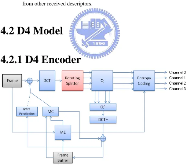
(24) 1.. Header information, such as SPS or PPS, carries the most important information to correctly decode the bit-stream and the bits needed to encode is almost negligible.. 2.. Intra macroblocks carry the key information that referenced by inter macroblocks, and with the intra block duplication, the side decoder reconstruction quality will better.. 3.. Motion vectors need less bits to encode than prediction error in most cases, but much more important. For example, in video sequences with less newly discovered objects, the temporal correlation is high, so that the error concealment of lost descriptors can have a good effect by motion vectors from other received descriptors.. 4.2 D4 Model 4.2.1 D4 Encoder. Figure 4.1. Encoder Architecture of D4 Model.. 16.

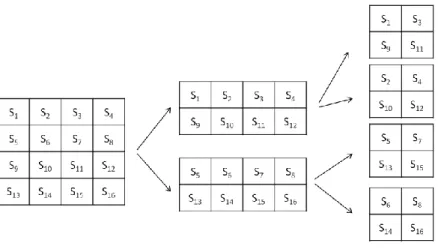
(25) D4 model splits the AC coefficients in an alternative rotating order. Figure 4.1 shows the overall encoder architecture of the D4 model. After the prediction error is transformed by integer DCT, the rotating splitter is performed. In Figure 4.1, except the rotating splitter block, which is between DCT and quantization block, all the other parts of the system are basically the same as conventional H.264/AVC encoding loop. There are four data paths output from the rotating splitter block, each path is for one descriptor and contains one-quarter of the original information, that is, one of every four consecutive AC coefficients in zig-zag scanning order is assigned to each descriptor. The detailed assignment algorithm will be introduced latter. After the quantization is performed, the quantized data on the four paths are separately entropy encoded to four bit-streams. The inverse quantization is performed on all four descriptors, and then the four split data paths are merged into a single one for reconstruction. The rotating splitter performs AC coefficient splitting based on the smallest block type in H.264/AVC: 4x4 block, since the integer DCT is a 4x4 2-dimensional transform, the splitting is based on 4x4 block. For each inter residual macroblock, 16 4x4 block are processed by rotating splitter in the order depicted in Figure 4.2.. Figure 4.2. 0. 1. 4. 5. 2. 3. 6. 7. 8. 9. 12. 13. 10. 11. 14. 15. 4x4 Block Processing Order in a Macroblock. 17.

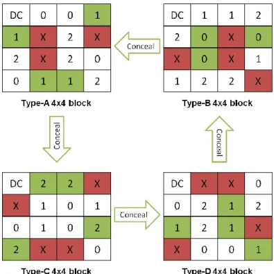
(26) We label the 15 AC coefficients in a 4x4 block with AC0, AC1, AC2….., AC15. Then, for each 4x4 block, the rotating splitter split the 15 AC coefficients in a way that alternatively assigned the coefficients to the four descriptors in the zig-zag scanning order: the first coefficient is assigned to the first descriptor and the second is assigned to the second …, etc. Figure 4.3 illustrates the assignment of each AC coefficient, and the number in the block is the descriptor number that the coefficient is assigned. Zig-zag order:. DC. AC0. 0. AC1. AC2. 1. 2. Figure 4.3. AC3. AC13. ‧‧‧. 3. AC14. 0. 1. AC15. 2. AC Coefficient Assignment in a 4x4 Block.. There is a problem in the alternative assignment algorithm, that is, the first descriptor always carries the lowest frequency coefficient in consecutive four coefficients, and the fourth descriptor carries the highest frequency coefficient. The lower frequency coefficients carry more energy, which is the characteristic of DCT, and is more important. As a result, the quality of the four descriptors will not be balanced: the first descriptor has the best quality, while the fourth descriptor has the lowest quality. The quality of each descriptor is not the same, which violates the principle of MDC discussed in chapter 1. To address the problem, the rotating splitter rotates the coefficient assignment among descriptors, thus generates four types of 4x4 block: A, B, C and D. Figure 4.4 illustrates the four types. The number in each block indicates the descriptor number that the coefficient is assigned. As Figure 4.4 shows, Type A begins by assigning AC0 to descriptor 0; type B assigns AC0 to descriptor 1; type C assigns AC0 to descriptor 2 and type D assigns AC0 to descriptor 3. The four types of 4x4 blocks are equally distributed inside each 16x16 macroblock in order to make the resulting descriptors 18.

(27) have balanced quality, as shown in Figure 4.5.. Figure 4.4. Four 4x4 Block Types the Rotating Splitter Generates. Figure 4.5. 4x4 Block Type Distribution in a Macroblock. Through this type of assignment, the error concealment described in the next sub-section can be utilized efficiently.. 4.2.2 Error Concealment in D4 The decoder is responsible for decoding and merging the received descriptors. The D4 decoding process of any one of the four descriptors is the same as that of the conventional H.264/AVC decoder, except the error concealment function which will be discussed later. When two or more descriptors are received, the decoder merges the coefficients before inverse DCT transform of a 4x4 block. This could be done by simply adding the coefficients in the same position from different descriptors. 19.

(28) For any lost descriptor, the error concealment is done by utilizing AC coefficient prediction through neighboring 4x4 blocks, since adjacent blocks have spatial correlation with each other. The coefficient prediction can take the advantage of the proposed 4x4 block type distribution shown in Figure 4.5, where since the types of adjacent 4x4 blocks are different, the coefficients in the same zig-zag order of neighboring blocks must belong to different descriptors and have very little chance to lose simultaneously. Therefore, error concealment is efficient through neighboring blocks. Figure 4.6 shows the prediction direction, which indicated by the four arrows. The lost coefficients in type-A are predicted from type-B block, the lost coefficients in type-B block are predicted from type-D block, and so on.. Figure 4.6. 4x4 Block Coefficient Prediction Direction. Figure 4.7 shows an example for error concealment of the lost descriptor 3. As we can see, the position labeled “X” means these coefficients are assigned to descriptor 3 and are lost. The left-top block is type A, and the lost coefficients in this block can be predicted from right-top block of type B, where the coefficients of the corresponding positions are assigned to descriptor 0, which is not lost, thus the three coefficient are copied from type-B block to type-A block. Similarily, the coefficients belonging to descriptor 1 in right-bottom type-D block are used to conceal the coefficients labeled „X‟ in type-B block, and etc.. 20.

(29) Figure 4.7. Coefficient Prediction and Descriptor 3 is Lost. 4.3 R4 Model 4.3.1 R4 Encoder Figure 4.8 shows another basic design of MDC model, called R4 model, which is also based on the principle discussed in chapter 3. The R4 model is a kind of residual domain splitting, that is, after the motion compensation, the “Res Splitter” will split the macroblock residual data into four macorblocks, one for each descriptor, and then transformed and quantized separately. As can be seen, the difference between R4 and D4 is that one performs the splitting before the DCT transformation, and the other after the transform.. 21.

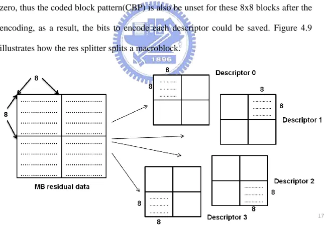
(30) Figure 4.8. Encoder Architecture of R4 Model. The 8x8 blocks that descriptors are not assigned, the residual data are set to all zero, thus the coded block pattern(CBP) is also be unset for these 8x8 blocks after the encoding, as a result, the bits to encode each descriptor could be saved. Figure 4.9 illustrates how the res splitter splits a macroblock.. Figure 4.9. Res Splitter Splits one Macroblock into Four Ones. In Figure 4.9, the residual data in a macroblock are divided into four by 8x8 blocks, each of them is be assigned to one descriptor. As the figure shows, the up-left 22.

(31) 8x8 block is assigned to descriptor 0; the up-right one is assigned to descriptor 1, etc. This makes each descriptor could at least set three bit in CPB to zero, so as to reduce to bit-rate for each descriptor. After res splitter, the encoding data path is split into four, and DCT transformation and quantization process becomes four times. The four data paths is are merged into one in the inverse quantization, because single prediction loop is used, and the full reconstruction of reference frames is needed. The R4 model follows the class A architecture described in chapter 2.. 4.3.2 Error Concealment in R4 Error concealment in R4 model is done in the residual domain by using the prediction of residual data through neighbor 8x8 blocks. In a macroblock, the residual data also has spatial correlation, thus it is benefit to utilize this property. The concealment algorithm is: for the lost 8x8 blocks, fill the residual data with the value x, which is the mean of the received residual data of the 8x8 blocks in the same macroblock. Figure 4.10 shows an example of error concealment of descriptor 3 loss.. Figure 4.10. An Macroblock Pattern After Loss Descriptor 3. In this case, the bottom-right 8x8 block is lost and all its residual pixels will be set to value 𝑓 , that is:. 23.

(32) 𝑓𝑗 ,𝑖 = 𝑓, 𝑓𝑜𝑟 8 ≤ 𝑗 ≤ 15 𝑎𝑛𝑑 8 ≤ 𝑖 ≤ 15. (4.1). where 1 𝑓= 8× 8× 3. 7. 7. 7. 15. 𝑓𝑗 ,𝑖 + 𝑗 =0 𝑖=0. 15. 7. 𝑓𝑗 ,𝑖 + 𝑗 =0 𝑖=8. 𝑓𝑗 ,𝑖 , 𝑓𝑗 ,𝑖 : 𝑟𝑒𝑠𝑖𝑑𝑢𝑎𝑙 𝑣𝑎𝑙𝑢𝑒 𝑗 =8 𝑖=0. 24. (4.2).

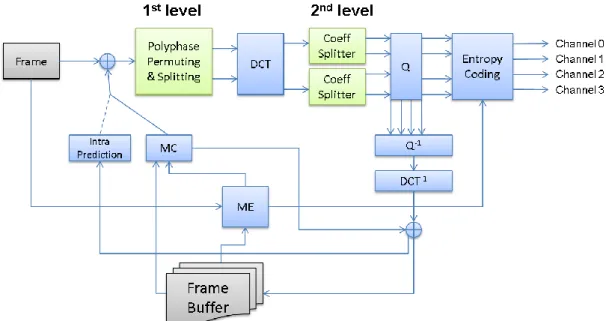
(33) Chapter 5 Hybrid Model. 5.1 Hybrid Encoder The basic models proposed in section 4.2 and 4.3 are able to meet the principle discussed in chapter 3, however, the splitting process in the encoders of both D4 and R4 do not take decoding process into considerations, thus, makes the decoder hard to effectively conceal lost descriptors. The performance in both bit-rate and reconstruction quality of D4 and R4 can be further improved if the design of encoder takes into account the concealment method used in the decoder.. Figure 5.1. Hybrid Encoder Architecture 25.

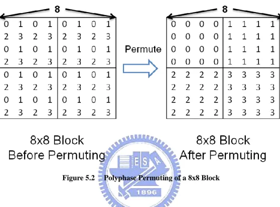
(34) In this section the hybrid model is proposed as an improved model based on the previous two models. Figure 5.1 shows the encoder architecture of the hybrid model. The encoder of hybrid model has a two-level splitting process in the encoding loop: 1) “Polyphase Permuting & Splitting” and 2) “Coeff Splitter”; the former is to split the block data in residual domain, and the latter is to split the transformed coefficients in frequency domain. Besides the two-level splitting, the remaining parts of the encoder are basically the same as conventional H.264/AVC encoder and the two basic models, except that the encoding path is split into two after the first-level splitting and then four paths after the second level splitting. The four paths are merged in the inverse quantization to reconstruct the full information of the reference frame, because, similar to D4 and R4, the Hybrid model adopts class A architecture which uses a single prediction loop. Other than the previous two basic models, the Hybrid model is designed to explore both the spatial correlation between adjacent pixel residual data and the frequency coefficient correlation between neighboring 4x4 blocks.. 5.1.1 Polyphase Permuting and Splitting The 1st level splitting, Polyphase Permuting and Splitting, is a spatial splitting in the residual domain, and is based on 8x8 block, that is, after motion compensation, the residual data in each 8x8 block will be polyphase permuted inside the block. The polyphase permutation is shown in Figure 4.12, where the left 8x8 block indicates the pixel index before permuting and the right one indicates that after permuting. The residual pixels in the 8x8 block are all labeled with a number from: 0, 1, 2, 3. The labeling mechanism is as shown in the figure that every four neighboring pixels, which is a matrix with 2x2 dimension, forms a group : 0 is on top-left, 1 is on 26.

(35) top-right, 2 is on bottom-left, 3 is on bottom-right, and there are 16 groups in a 8x8 block. The polyphase permuting then rearranges the top-left pixel of each group to the top-left 4x4 block, top-right pixel of each group to the top-right 4x4 block, etc.. Figure 5.2. Polyphase Permuting of a 8x8 Block. After permuting, the pixels labeled with the same number are grouped into the same 4x4 block, as shown in right 8x8 block of Figure 5.2, in which the block is partitioned into four 4x4 block. The four 8x8 blocks in each macroblocks are all permuted in the same way. The splitting process is then performed the permuted macroblocks. The splitting process is shown in Figure 5.3. A 8x8 block is split into two 8x8 blocks, called residual 0 (R0) and residual 1 (R1), each carries two 4x4 residual blocks chosen in diagonal: top-left and bottom-right 4x4 residual blocks are in one 8x8 block, while top-right and bottom-left ones are in the other 8x8 block. For each 8x8 block, the remaining two 4x4 blocks with pixels all labeled with „x‟ in the figure are given residual pixels all set to zero, thus form all-zero blocks. The encoder needs 27.

(36) not to encode the coefficient of these two all-zero 4x4 blocks. The reason to permute pixels inside the 8x8 block before splitting is to take the advantage of interpolation in the decoder error concealment, which will be discussed in later sections.. Figure 5.3. Splitting of a 8x8 Block. The encoding path in Figure 5.1 is split into two after the 1st level splitting; for each path, the DCT is then applied to every 4x4 block, resulting in twice the transformation process. However, since half the total number of 4x4 blocks are all-zero blocks, which essentially need not to be transformed, thus the transformation time can be reduced by skipping the transformation of the all-zero blocks. After the transformation, the 2nd level splitting, “Coeff Splitter,” is to split the frequency domain coefficients.. 5.1.2 Coeff Splitter 28.

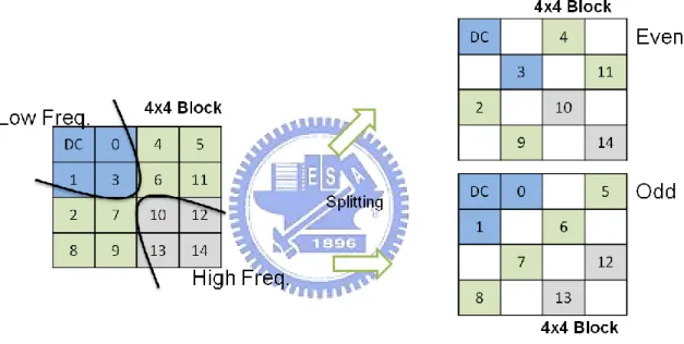
(37) The 2nd level splitting, Coeff Splitter, is based on splitting of the DCT AC coefficients in the frequency domain. It is modified from the D4 model. In the coefficient splitting of D4 model, the coefficients are assigned to each one of the four descriptors alternatively as discussed in section 4.1, which may resulting in an unbalanced qualities of descriptors, while in the hybrid model, the coefficient splitting process is modified to improve this drawback. It is known that DCT coefficients have different importance in human‟s subjective visual quality. The coefficients of lower frequency are more important, because they are more sensitive to human visual system, while coefficients of higher frequency are generally less important. Thus, the “Coeff Splitter” takes into account the different importance of DCT coefficients.. Figure 5.4. Groups of Frequency in 4x4 Block. The 16 DCT coefficients in a transformed 4x4 block are divided into three groups: 1) low frequency, 2) median frequency, 3) high frequency, as shown in Figure 5.4: the four coefficients that are closest to DC are assigned to low frequency group, that is DC, AC0, AC1, AC3. The four coefficients that are furthest to DC are assigned to high frequency group, that is AC10, AC12, AC13, AC14. Other coefficients are in the median frequency group. 29.

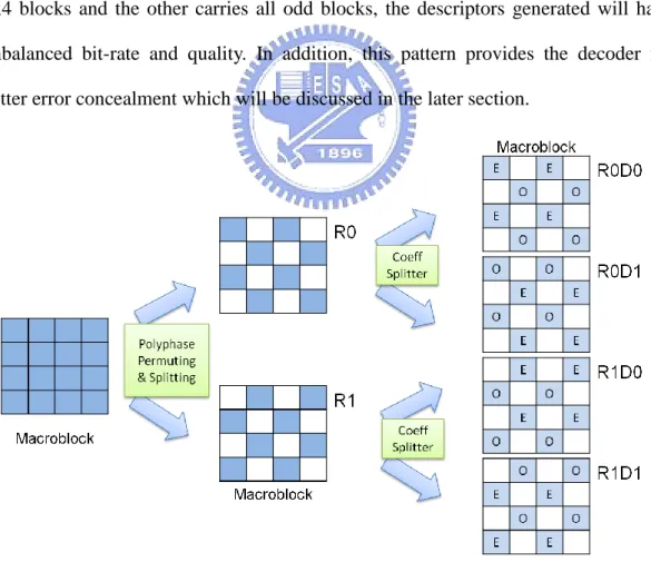
(38) Based on the grouping strategy, the Coeff Splitter splits the AC coefficients of each group to two descriptors. The DC is duplicated to each descriptor, since DC is the most important. Figure 5.5 shows a 4x4 block which is split into two 4x4 blocks, each carries almost half the total number of original coefficients. The 4x4 block which carries even number of original AC coefficients is calles even block, while the other block is called odd block. Besides the DC which is duplicated to both blocks, each AC group is divided in diagonal direction in order to achieve a balanced visual quality.. Figure 5.5. Even and Odd 4x4 Blocks Are Generated by Coeff Splitter. As the figure shows, every other top-right to bottom-left diagonal of coefficients are assigned to the same descriptor, resulting in a reduced number of (Run, Level) pairs for each descriptor and therefore entropy encoding, such as, CABAC or CAVLC, will be more effective. The two type of 4x4 blocks: odd and even, will be assigned to two descriptors in an alternative diagonal pattern, as illustrated in Figure 5.6.. In Figure 5.6, a residual macroblock after motion compensation is first split into two macroblocks, called R0 and R1. The white color blocks in R0 and R1 are all-zero 30.

(39) 4x4 blocks. Then, for each split macroblock, Coeff Splitter is applied to split every non-zero 4x4 block into odd and even blocks and alternatively assigned to two different macroblocks, labeled D0 and D1 in Figure 5.6, where the D0 and D1coming from R0 are also called R0D0 and R0D1, respectively, and those from R1 are called R1D0 and R1D1, respectively. As a result, for every residual macroblocks in the motion compensation frame, four macroblocks (R0D0, R0D1, R1D0 and R1D1) are generated for four descriptors. The purpose of assigning the even and odd macroblocks in an alternative diagonal pattern is to balance the difference in the even and odd blocks, since the odd blocks have one more coefficients than the even blocks. If a descriptor carries all even 4x4 blocks and the other carries all odd blocks, the descriptors generated will have unbalanced bit-rate and quality. In addition, this pattern provides the decoder for better error concealment which will be discussed in the later section.. Figure 5.6. Macroblock Pattern After Two Level Splitting. From Figure 5.1 and Figure 5.6, the encoding process of a macroblock is shown: a macroblock is split to four descriptors, and then the four split macroblocks are 31.

(40) mergeed in the inverse quantizaton process so as to reconstruct the full information frame for motion estimation. The same to R4 and D4 models, the Hybrid model follows the MDC criterion discussed in chapter 3, and adopts class A architecture which uses a single prediction loop.. 5.1.3 Frequency and Spatial Merge. Figure 5.7. The Coeff Merger in Frequency Domain. The top three 4x4 blocks in Figure 5.9 shows the Coeff Merger of even and odd blocks in frequency domain. The merging is done by adding ACs in the same positions of even and odd blocks to form the original 4x4 block and one of the two duplicated DCs is chosen. The bottom two shows macroblocks after merging all the 4x4 blocks in the macroblock, the left one is resulting from merge of R0D0 and R0D1, and the other is from R1D0 and R1D1. After inverse transformed to residual pixels, R0 and R1 are obtained and then the 2nd level merging is applied. Figure 5.8 illustrates the merging process.. 32.

(41) Figure 5.8. The Residual Merging and Polyphase Inverse Permutation. Instead of using 4x4 block, the 2nd level merging is based on 8x8 block. The residual pixels labeled „x‟ in the left two 8x8 blocks are zeroes, which will be discarded and result in one 8x8 block after merging. This 8x8 block is then polyphase inverse permuted to reconstruct the original 8x8 block, as shown in the right side of Figure 5.8. For each macroblock, all the four 8x8 blocks will be applied in this process.. 5.2 Hybrid Decoder The decoder system architecture of the Hybrid model is shown in Figure 5.9. The four descriptors are labeled with R0D0, R0D1, R1D0 and R1D1; R0D0 and R0D1 are split from R0; R1D0 and R1D1 are split from R1. These descriptors are first entropy decoded separately and then “Coeff Merger” and “Residual Merge & Polyphase Inverse Permuting” are performed, the same as in the encoder. If descriptors lost, then depending on the received descriptor pattern, either frequency concealment or spatial concealment will be applied to error concealment. If 33.

(42) the received descriptors are in the same residual domain, for example, R0D0 and R0D1 that are in R0, the spatial concealment is applied, and if the both residual domain have descriptors received, for example, R0D0 and R0D1, in this case, the frequency concealment will be applied. The detailed concealment algorithm is discussed in later sections.. Figure 5.9. Descriptor State Residual Domain 1 (R1) Table 5.1. Hybrid Decoder Architecture. Residual Domain 0 (R0) D0+D1. D0+D1. D0. D1. Loss. F. F. S. D0. F. F. F. S. D1. F. F. F. S. Loss. S. S. S. Summary of Spatial and Frequency Concealment Cases. Table 5.1 summaries the cases for spatial or frequency concealment to be applied; 34.

(43) F denotes frequency concealment, and S denotes spatial concealment. The D0+D1 column means the two descriptors generated from R0 are received; while the D0 column and D1 column mean only one of the two descriptors is received. Loss column means no descriptor from R0 is obtained. The D0 and D1 in rows mean the descriptors are from R1. As can be seen, the spatial concealment is applied only when one descriptor is received or two from the same residual domain are received; while other cases the frequency concealment is utilized.. 5.2.1 Spatial Concealment Figure 5.10 and Figure 5.11 illustrates the cases that spatial concealment is performed, where Figure 5.10 illustrates four cases that only one descriptor is received; while Figure 5.11 depicted the two cases that two descriptors in the same residual domain are received. R0‟ and R1‟ are the concealed version of R0 and R1, respectively.. Figure 5.10. Spatial Concealment for One Received Descriptor. 35.

(44) Figure 5.11. Spatial Concealment for Two Received Descriptors. For each case in Figure 5.10 and 5.11, only one of the R0 and R1 can be constructed or partially constructed from the received descriptors, and the other one is totally lost. Here we propose to obtain the lost one by using spatial concealment. Figure 5.13 is an example where R0 has been constructed by the received descriptors, but R1 is totally lost. Note that the black area is actually the information carried by R1. After the polyphase inverse permutation of R0, the constructed residual pixels are distributed like a check board in the macroblock. For each lost residual pixel, there are four available neighboring pixels, which have high spatial correlation to the lost residual pixel and therefore spatial concealment can be utilized.. Figure 5.12. Spatial Concealment by Bilinear Interpolation. 𝑓j,i = 𝑓j+1,i + 𝑓j−1,i + 𝑓j,i+1 + 𝑓j,i−1. 4. (4.3). The spatial concealment utilizes the bilinear interpolation to conceal the lost 36.

(45) residual pixels. Equation 4.3 is the bilinear interpolation algorithm. 𝑓j,i is the concealed residual pixel value, and the north, west, south and west neighboring pixels are all referenced.. 5.2.2 Frequency Concealment The frequency concealment is done by the prediction of the AC coefficients through the blocks in the center part of the residual domain. Due to the polyphase permutation, the four 4x4 blocks can the viewed as the scaling-down sub-image by factor two in width and height of the contained 8x8 block. As a result, the four blocks are similar and the transformed coefficients should have higher correlation. Thus, the prediction of AC among these correlated blocks is efficient. Since even and odd blocks contain complementary coefficient information, the AC prediction follows the principle: even block predict from odd and odd block predict from even; that is, the lost coefficients in an even block will copied from the same position of a chosen odd block, called prediction block, and vice versa. The choice of prediction block depends on the descriptor receiving pattern. Figure 5.13 shows four cases of receiving two descriptors and the dotted arrows represent the prediction direction in a maroblock of each case. The right macroblocks in (a), (b), (c) and (d) illustrate the concealment pattern of each of the 16 4x4 block type, „E‟ denotes even type, and „O‟ denotes odd type. With the design of 2nd level splitting in the Hybrid encoder, the diagonal 4x4 blocks have different types in each 8x8 block, resulting in two prediction directions: horizontal and vertical; (a) and (b) are in horizontal, while (c) and (d) are vertical in the figure.. 37.

(46) Figure 5.13. AC Prediction for Two Received Descriptors. In Figure 5.13 (a) and (b), the received two descriptors are in different residual domain and in different frequency domain, which makes the macroblock form columns of even blocks and columns of odd blocks, thus the prediction block is chosen in horizontal direction, while in (c) and (d), the received descriptors are in the same frequency domain, that is both are D0 or both are D1, which makes the macroblock rows of even blocks and rows of odd blocks, thus the prediction block is chosen in vertical direction.. Figure 5.14. AC Prediction for Three Received Descriptors. Figure 5.14 illustrates the four cases of receiving three descriptors with the 38.

(47) dotted arrows representing the prediction directions. Since three descriptors are received, there is one residual domain can be fully reconstructed, either R0 or R1, only the other residual domain need to be concealed, in other words, 8 of the 16 4x4 blocks in a macroblock need AC prediction. The prediction block direction is as shown in the figure, and all cases are similar that only horizontal direction is applied. The frequency concealment in previous section is based on prediction of AC coefficients from corresponding or neighboring block in the counterpart of the residual domain. However, the effect of AC prediction varies according to the number of predicted AC coefficients. The following figures show the experimental results for the quality of different sequences by varying different number of predicted AC coefficients. The experiment is based on receiving two descriptors and utilizing the frequency concealment.. Figure 5.15. Results of Qualities by Varying Number of Concealed ACs. 39.

(48) In Figure 5.15, the x-axis is the number of ACs used for concealment, ranged from 0 to 15, 0 stands for no concealment, and 15 means that all AC coefficients are copied from the predicted 4x4 block. In addition, the concealment is according to the zig-zag scanning order, which means that if the number of AC for concealment is k, then for every lost 4x4 block, only first k ACs in zig-zag order will be copied from a the corresponding predicted blocks. From Figure 5.15, it can be observe that the peak of quality is in the interval [3,5] in most sequences. There are two local maximum in the foreman sequence though, however, one of them also falls in the interval [3,5]. Therefore, we choose 4 as the number of AC coefficients for concealment.. 40.

(49) Chapter 6 Experimental Results. In this chapter, the experimental results of the four models: PSS [7], D4, R4 and Hybrid, are presented, and five test sequences: foreman, mobile, coastguard, carphone, news, with QCIF (176x144) resolution are used for performance evaluation. These models are implemented in H.264/AVC reference software, JM 13.2 [15]. The group of picture (GOP) size is 20 frames. The type of each GOP is IPPP…, the frame rate is set to 30 Hz, and the symbol mode is set to CABAC. The performance is measured by the reconstruction quality of 1, 2 and 3 descriptors and their corresponding bit-rate and overall redundancy rate, R*, defined in equation 5.1. The quality variation of each frame is also provided for each model. Equation 5.1 is the redundancy rate, R(R0D0) stands for the bit-rate of the descriptor R0D0, and R(SD) is the bit-rate of SDC under the same QP.. 𝑅∗ =. 𝑅 𝑀𝐷𝐶 𝑚𝑜𝑑𝑒𝑙. (6.1). 𝑅(𝑆𝐷). , where MDC model can be PSS, D4, R4 or Hybrid, and R(SD) is the bit-rate of standard H.264/AVC with the same QP of the above MDC models. The experiments use Peak Signal-to-Noise Ratio (PSNR) for measuring the quality of reconstructed sequences. Equation (5.2) defines the PSNR. 41.

(50) 𝑃𝑆𝑁𝑅 = 10 × 𝑙𝑜𝑔. 255 2. (6.2). 𝑀𝑆𝐸. , where. 𝑀𝑆𝐸 =. 𝑕 𝑒𝑖𝑔 𝑕 𝑡 𝑗 =1. 𝑤𝑖𝑑𝑡 𝑕 𝑖=1. 𝑓 𝑗 ,𝑖 −𝑓𝑗 ,𝑖. 2. (6.3). 𝑕𝑒𝑖𝑔 𝑕𝑡× 𝑤𝑖𝑑𝑡 𝑕. Height and width are the frame resolution; 𝑓𝑗 ,𝑖 is the pixel value of the original sequence and 𝑓𝑗 ,𝑖 is the reconstructed pixel value in the decoder.. 6.1 Three Descriptors The first experiment is conducted under the situation that only one out of the four descriptors is lost, that is, three descriptors are received for each stream. Figure 6.1 shows the reconstructed PSNR of (a) foreman, (b) carphone and (c) coastguard for different bit-rates. Since there are four possible cases in one descriptor loss, that is, one from the four descriptors, the reconstructed PSNR is the average of the four cases.. (a). 42.

(51) (b). (c). Figure 6.1. PSNR of Three Received Descriptors at Different Bit-rates. (a) Foreman. (b) Carphone. (c) Coastguard.. It is observed that in (a) and (b), the Hybrid model has a higher PSNR, ranged from 1 to 2 dB than other models in low to high bit-rates. However, at high bit-rate in (c), which is the coastguard sequence, the PSNR of the PSS is higher than the Hybrid and the PSNR difference of the Hybrid and other models is smaller, about 0.5. Since 43.

(52) there are more new object that show up during the sequence, resulting in more intra coded blocks and a higher redundancy, and the error concealment of PSS model utilizes a gradient calculation which is more effective for the content of the coastguard, which has horizontal coastline, ships and waves. Figure 6.2 shows the PSNR of each reconstructed frame of different sequences and the first 100 frames with 5 GOPs are shown in the figure.. (a). (b). 44.

(53) (c). Figure 6.2. PSNR of Each Frame of Receiving Three Descriptors. (a) Foreman. (b) Carphone. (c) Coastguard.. Note that in D4, R4 and Hybrid models, the intra coded macroblocks are duplicated to each of the four descriptors thus for each descriptor the intra frame will contains full information. That is, the intra frame can be reconstructed with full quality in case of some descriptor loss. However, for each other frame inside the GOP, the quality is degraded due to descriptor loss. The degradation is propagated to the end of the GOP, that is, before the next intra frame is reconstructed. It is observed that class B models, D4, R4 and Hybrid, have periodical degradation for each GOP, while in PSS, it is the PSNR depends on the effect of edge sensing algorithm. In addition, in (a) and (b) the Hybrid model almost has better PSNR for every frame in each GOP than other models, however in (c), PSS has better PSNR in the first two GOP and a similar PSNR in the third GOP, and the Hybrid model is better in the following GOPs, since in the coastguard sequence, there is a ship coming into the picture and in the later GOPs, the ship is fully in the picture. Table 6.1 shows the PSNR of each model at 100 Kbit/s, which is a median bit-rate in the experiment. The difference of PSNR between models is not large compared to the following cases that will be discussed in the following section. The 45.

(54) Hybrid model is 0.65 to 1.77 higher than other models.. Table 6.1. Quality of Each Model at 100 Kbit/s per Descriptor.. The R* of foreman, carphone and coastguard are 3.14, 2.28 and 2.19, respectively.. 6.2 Two Descriptors The second experiment is conducted under the situation that two descriptors are received for each stream. Figure 6.3 shows the reconstructed PSNR of (a) foreman, (b) carphone and (c) coastguard for different bit-rates. Since there are six possible cases that two from the four descriptors loss, the reconstructed PSNR is the average of the six cases. (a). 46.

(55) (b). (c). Figure 6.3. PSNR of Two Received Descriptors at Different Bit-rates. (a) Foreman. (b) Carphone. (c) Coastguard.. In Figure 6.3, the Hybrid model has better performance for low bit-rate to high bit-rate in every sequence, since the spatial concealment and frequency concealment 47.

(56) are effective than other models in this case. Basically, R4 and D4 have similar behavior of receiving one and two descriptors in the carphone sequence. The PSS model has a better performance in coastguard sequence than other sequences, as discussed in previous section. The receiving two descriptors case is less effective than receiving three descriptors, since the concealment in the decoder of the PSS model utilizes bilinear interpolator, other than the edge sensing algorithm, which has better performance, used in receiving three descriptors case.. (a). (b). 48.

(57) (c). Figure 6.4. PSNR of Each Frame of Receiving Two Descriptors. (a) Foreman. (b) Carphone. (c) Coastguard.. Figure 6.4 shows the PSNR of each reconstructed frame of different sequences and the first 100 frames with 5 GOPs are shown in the figure. Similar to previous section, each GOP has degradation in class A models, D4, R4 and Hybrid. Basically, even there degradation in each GOP, the PSNR of the Hybrid model of each frame is higher than other models, besides the tail frames in the first two GOPs in the coastguard sequence, as discussed in previous section. The PSS model is a class B model, which controls mismatch, and has not degradation in a GOP. However, the coding efficiency becomes inefficient; PSNR of every frame in each GOP is lower than the Hybrid model and the number of frames that have higher PSNR than D4 or R4 models becomes lesser. Table 6.1 shows the PSNR of each model at 100 Kbit/s, which is a median bit-rate in the experiment. Through the same bit-rate, the PSNR of each model shown in numerical can be compared more accurately. The Hybrid model has at least 1.4 ~ 3.4 dB higher PSNR in the receiving two descriptors case which is better than the previous section. 49.

(58) Table 6.2. Quality of Each Model at 100 Kbit/s.. The R* of foreman, carphone and coastguard are 3.14, 2.28 and 2.19, respectively.. 6.3 One Descriptor The third experiment is conducted under the situation that only one descriptor is received for each stream. Figure 6.5 shows the reconstructed PSNR of (a) foreman, (b) carphone and (c) coastguard for different bit-rates. There are four possible cases that one from the four descriptors loss, so the reconstructed PSNR is the average of the four cases.. (a). 50.

(59) (b). (c). Figure 6.5. PSNR of One Received Descriptors at Different Bit-rates. (a) Foreman. (b) Carphone. (c) Coastguard.. In Figure 6.5, it is observed that the curves of each model is separate and has no crosses, which means the increasing of bit-rate has limited effect for higher PSNR. There is large difference between the performance of PSS and other models, since the 51.

(60) error concealment of PSS uses near-neighbor replicator (NNR), which has poor effect. In the receiving one descriptor case, the Hybrid model has obviously higher performance than other models, because even in receiving one descriptor, the error concealment can still utilize bilinear interpolator, while in other models, the spatial or frequency distance is too far to make effective concealment.. (a). (b). 52.

(61) (c). Figure 6.6. PSNR of Each Frame of Receiving One Descriptor.. (a) Foreman. (b) Carphone. (c) Coastguard.. Figure 6.6 shows the PSNR of each reconstructed frame of different sequences and the first 100 frames with 5 GOPs are shown in the figure. The curves in the figure are separate, and the difference performance of each model is stable. In this case, there is also degradation of PSNR in a GOP, though the PSNR of each frame of the Hybrid model is higher than other models. In (b) and (c), the performance of D4 and R4 similar frame-by-frame, in accordance to the result which is shown in Figure 6.5 (b) and (c). The curve of the PSS model is stable and low, because the limited effect of NNR algorithm. In the receiving one descriptor case, the Hybrid model has a higher performance than the cases discussed in the previous two sections, due to the effective error concealment in the decoder. Table 6.3 illustrates the numerical result comparison, and the Hybrid model is 1.19 ~ 7.77 dB higher in PSNR than other models. As discussed previously, the effect of NNR algorithm in the PSS model can be observed by the table.. 53.

(62) Table 6.3. Quality of Each Model at 100 Kbit/s.. The R* of foreman, carphone and coastguard are 3.14, 2.28 and 2.19, respectively.. 6.4 Packet Loss Simulation In some circumstances, the descriptors will not loss entirely, but lost part of packets in the transmission of each descriptor. In this section, the performance of each model in the burst packet loss environment is provided with packet lost one descriptor and simultaneously lost in two and three descriptors. Figure 6.7 illustrates the PSNR degradation of each model when packet loss occurs in one (a), two (b) and three (c) descriptors at the 42th frame.. (a). 54.

(63) (b). (c). Figure 6.7. PSNR Degradation of Packet Lost in Descriptors. (a) One Descirptor. (b) Two Descriptors. (c) Three Descriptors.. It is observed that the first frame after packet loss has the largest PSNR degradation in each model, and then the degradation is reduced gradually, and in the 61th frame the PSNR stops degrading since 61th frame is the intra frame of the next GOP. As in the previous sections about descriptors loss, the PSS model has poor performance in the experiment, especially in the packet loss simultaneously in three descriptors. The degradation of the Hybrid model is lower than other models in all three cases, so the model has a more robust error resilience capability.. 55.

(64) Chapter 7 Conclusion. A hybrid model of multiple description coding had been proposed. The splitting process in the encoder is divided to two stages: the first stage splits the residual data in spatial domain, and the second stage splits the AC coefficients in the frequency domain. In the decoder, the two type of error concealment, which utilize spatial correlation between residual pixels and frequency correlation between adjacent blocks, is proposed to improve the reconstruction quality when descriptors loss. Through the design of encoder, error concealment in the decoder is more effective, even when only one or two descriptors received. According to the experimental results, it is observed that, compared with the three descriptors received cases, in the one or two descriptors received case, the Hybrid model is more effective than other models. No matter in receiving one, two or three descriptors cases, the Hybrid model can make a effective error concealment, other than D4, R4 and PSS models, which have better performance in receiving three descriptors case and have obviously less effective performance in the receiving one and two descriptors cases.. 56.

(65) Reference [1] A. Vetro, J. Xin, H. Sun, "Error Resillence Video Transcoding for Wireless Communications", IEEE Wireless Communications , Vol. 12, Issue 4, pp. 14-21, Aug. 2005. [2] V. K. Goyal, "Multiple Description Coding: Compression Meets the Network," IEEE Signal Processing Magazine, vol. 18, no. 5, Sept. 2001. [3] Y. Wang, A. R. Reibman, and S. Lin, “Multiple Description Coding for Video Delivery,” Proceeding IEEE, vol. 93, no. 1, Jan. 2005. [4] V.A. Vaishampayan, “Design of Multiple Description Scalar Quantizers,” IEEE Transaction on Information Theory, vol. 39, 1993. [5] J. Apostolopoulos, W. Tan, S.J.Wee, and G.W. Wornell, “Modeling Path Diversity for Multiple Description Video Communication,” IEEE International Conference on Acoustics, Speech, and Signal Processing (ICASSP), May 2002. [6] O. Campana, R. Contiero, “An H.264/AVC Video Coder Based on Multiple Description Scalar Quantizer,” IEEE Asilomar Conference on Signals, Systems and Computers(ACSSC), 2006. [7] R. Bemardini, M. Durigon, R. Rinaldo, L. Celetto, and A. Vitali, “Polyphase Spatial Subsampling Multiple Description Coding of Video Streams with H.264,” Proceedings of IEEE International Conference on Image Processing(ICIP), Oct. 2004. [8] A. Reibman, H. Jafarkhani, Y. Wang, M. Orchard, “Multiple Description Video Using Rate-Distortion Splitting,” Proceedings of IEEE International Conference on Image Processing(ICIP), 2001. [9] Matty, K.R. and Kondi, L.P., “Balanced multiple description video coding using 57.

(66) optimal partitioning of the DCT coefficients,” IEEE Transaction on Circuits and Systems for Video Technology, vol. 15, no. 7, July 2005. [10] Nicola Conci, Francesco G.B. Natale, “Multiple Description Video Coding Using Coefficients Ordering and Interpolation,” Signal Processing: Image Communication, 2007. [11] J. Jia and H. K. Kim, “Polyphase Downsampling Based Multiple Description Coding Applied to H.264 Video Coding,” IEICE Transactions, June 2006. [12] J. G. Apostolopoulos, “Error-Resilient Video Compression Through the Use of Multiple States,” in ICIP00, vol. 3, 2000. [13] S. Gao, H. Gharavi, “Multiple Description Video Coding over Multiple Path Routing Networks,” International Conference on Digital Communication Proceedings(ICDT), 2006. [14] D. Wang, N. Canagarajah and D. Bull, “Slice Group Based Multiple Description Video Coding Using Motion Vector Estimation,” IEEE International Conference on Image Processing(ICIP), 2004. [15] H.264/AVC Reference Software – JM 13.2, http://iphome.hhi.de/suehring/tml/.. 58.

(67)