光學玻璃模造成形之有限元素分析

(1)

國

立

交

通

大

學

機械工程學系

博士

論

文

光學玻璃模造成形之有限元素分析

Finite Element Analysis on the Optical Glass Molding Process

研究生：蔡宇中

指導教授：洪景華教授

(2)

光學玻璃模造成形之有限元素分析

Finite Element Analysis on the Optical Glass Molding Process

研究生：蔡宇中 Student：Yu-Chung Tsai

指導教授：洪景華 Advisor：Chinghua Hung

國立交通大學

機械工程學系

博士論文

A Dissertation

Submitted to Department of Mechanical Engineering College of Engineering

National Chiao Tung University in partial Fulfillment of the Requirements

for the Degree of Doctor of Philosophy in Mechanical Engineering June 2010 Hsinchu, Taiwan

中華民國九十九年六月

(3)

i

光學玻璃模造成形之有限元素分析

研究生

: 蔡宇中指導教授: 洪景華教授

國立交通大學機械工程學系

摘要

玻璃模造技術為一適合用於大量製造內嵌在 3C 產品中的光學元件(如手機相機模組中的光學玻璃透鏡)之量產方式。儘管此技術具備許多優勢，在實際製造上仍有許多困難需克服。其中最關鍵的問題為歷經製程後的透鏡成品與原始設計值之間存在誤差。為解決此問題，本研究以詳盡的材料模型建立有限元素分析模型，並以此模型預測光學玻璃模造後之透鏡成品外型，期能藉此分析指出此問題關鍵處並加以改善。為建構一完整的光學玻璃模造成形之有限元素分析模型，本研究一開始即針對玻璃進行材料實驗以取得詳盡的材料性質。研究裡採用的是低玻璃轉移溫度之玻璃L-BAL42 (Low T_g glass, T_g=506°C, Ohara Co.)。藉由熱膨脹實驗，得到玻璃在液體和玻璃態下的熱膨脹係數。接著利用掃描式熱差分儀（DSC）和單軸壓縮應力鬆弛實驗，分別取得玻璃之結構鬆弛性質以及應力鬆弛性質。另在成形溫度（568℃，At + 30℃）下進行單軸壓縮試驗，驗證牛頓流體確實能夠準確地代表玻璃在成形階段的流動行為。最後進行一非球面光學玻璃透鏡成形實驗，並以此實驗之成形參數代入分析中。分析模型以商用有限元素軟體 MARC 建立，並代入玻璃材料實驗所得之材料性質。藉由模擬和實驗結果比對一致性與準確性，確認了本研究提出之光學玻璃模造成形有限元素分析模型。

(4)

ii

關鍵字: 光學玻璃透鏡，玻璃模造成形，有限元素分析，熱膨脹，單軸壓縮，牛 頓流體，結構鬆弛，應力鬆弛。

(5)

iii

FINITE ELEMENT ANALYSIS ON THE OPTICAL

GLASS MOLDING PROCESS

Student: Yu-Chung Tsai

Advisor: Prof. Chinghua Hung

Department of Mechanical Engineering

National Chiao Tung University

ABSTRACT

Glass molding is a high-volume fabrication method suitable for producing optical components embedded in 3C products, such as optical glass lenses in the camera modules of mobile phones, digital cameras and projectors, etc. Despite the advantages of glass molding, several difficulties encountered in the manufacturing process have yet to be overcome. The most critical issue is the deviation between the formed lens and the original lens shape design. Thus, to overcome this obstacle, the focus of this dissertation is to introduce finite element analysis (FEA) into the prediction of the molded lens shape with detailed material models of the optical glass.

To construct a comprehensive finite element (FE) model for the optical glass molding process, this study firstly performed experiments on the optical glass to obtain detailed material properties. Low Tg optical glass, L-BAL42 (Tg=506°C, Ohara

Co.), was used in this research. Detailed thermal expansion coefficients including liquid and glassy states are obtained by thermal expansion experiment. Followed by using differential scanning calorimetry (DSC) and uniaxial compressive stress relaxation experiments, the structural relaxation property and the stress relaxation property were obtained respectively. Uniaxial compression test was also performed at

(6)

iv

the molding temperature (568°C, 30°C above At) to verify that the Newtonian fluid could accurately represent the glass flow behavior at molding stage. An aspherical optical glass lens molding experiment was then performed and the FEA with the same forming parameters was also conducted by using the commercial finite element program, MARC, incorporating these obtained material properties and the proposed material model. After verifying the consistency of simulation and experimental results, a comprehensive FE model for optical glass lens molding process was assured.

Keywords: Optical glass lens, glass molding, finite element, thermal expansion,

(7)

v

誌謝

首先要感謝指導教授，洪景華老師，從我碩士班一路到博士班，一共九年的時光，不厭其煩、不辭辛勞的在研究的路途上引導我，在研究過程中各個關鍵時刻拉拔我，讓我順利完成學業，邁入人生下一個階段。遇到一個這麼好的師父，是我這一生中最幸運的一件事。非常感謝口試委員黃佑民教授、徐瑞坤教授、宋震國教授、賀陳弘教授和黃國政博士。感謝你們提出的諸多建議，讓我的論文更臻完整。儀科中心曾釋鋒先生、黃建堯先生、郭朝輝先生，非常感謝三位在百忙中仍抽空協助我進行實驗，讓我能順利完成研究。感謝洪榮崇學長，不但在研究上提供實驗機台和許多寶貴的建議，在研究之外也不忘照顧我、提點我，讓我這九年的求學之路走得更為順遂。除了父母之外，最照顧我的，當屬待我如親兄弟的洪榮崇學長了。實驗室的學弟妹們:雅雯、建溢、奇忠、政成、琇晶、維德、智偉、煌棊、正展、銘傑、麒禎、嘉偉、理強、宗駿、彥彬、黃詠、世璿、運賢、志嘉、俊羿、志傑、聖平、時恆、建榮、麒翔、忠諭、宗錞、筱瑋、立釗、正一、振傑、雅喬、中南、書麟、馨云。感謝你們多年來一直容忍我作威作福，對你們做出各式威脅逼迫的動作。恭喜你們，終於脫離威權，迎向民權了! 交大十三年，研究所九年，一路走來雖有些許顛簸，但仍算極為順遂。特別是路途中遇到的諸多貴人，讓我無論在研究上或生活上都能順利過關。對於諸位，在此僅以感恩二字表達最衷心的感激之意。最後，非常感激我的家人，特別是我的父母，在我的求學過程中無怨無悔的支持我，給我最大的自由度去探索這個世界。非常榮幸能作你們的兒子，感謝你們!

(8)

vi

LIST OF TABLES

Table 3.1 Structural relaxation parameters used in the FEA. ... 46

Table 3.2 Stress relaxation parameters used in the FEA. ... 46

Table 4.1 Coefficients of aspherical surfaces. ... 75

Table 4.2 Mechanical and thermal properties of glass [35] and molds [36]. ... 75

Table 4.3 Lens shape differences between experimental and experimental results ... 75

Table 4.4 Surface curve deviations between experimental and FEA results. ... 76

Table 4.5 RMS values of the surface curve deviations between experimental and FEA results (with and without stress and structural relaxation). ... 76

Table 4.6 Central thickness of the formed lens under various molding forces and molding times. ... 76

Table 4.7 Diameter of the formed lens under various molding forces and molding times. ... 77

Table 4.8 FEA results with different cooling rates (diameter and central thickness of the formed lens). ... 77

(11)

ix

LIST OF FIGURES

Figure 1.1 Cup shape diamond grinding tool conducting (a) concave (b) convex (c)

multi-lens pre-forming process [1]. ... 7

Figure 1.2 Schema of the traditional polishing process [2] ... 7

Figure 1.3 (a) Schema of the spherical aberration in a spherical lens (b) Lens group for eliminating spherical aberration [3]. ... 8

Figure 1.4 Aspherical lens focusing the collimating lights on a single point of the lens axis [4]. ... 8

Figure 1.5 Schema of the optical glass molding process. ... 9

Figure 1.6 Schema of the optical glass molding history ... 9

Figure 1.7 Various optical lenses (Bi-convex lens, Bi-concave lens, Ball lens, Meniscus lens, Insertion lens, f-θ lens, Micro lens array, Fiber array) fabricated by optical glass molding technology (Toshiba Machine Co.) [6]. ... 10

Figure 2.1 Typical curve for viscosity as a function of temperature for a commercial soda-lime-silicate glass [19]... 21

Figure 2.2 Standard points of L-BAL42 and the fitted viscosity curve (by VFT equation). ... 21

Figure 2.3 Thermal expansion curve of a typical optical glass [20]. ... 22

Figure 2.4 Commonly used viscoelastic models (a) Maxwell model (b) Kevin-Voigt model. ... 23

Figure 2.5 Stress response to applied constant strain (Maxwell model) [21]. ... 23

Figure 2.6 Strain response to applied stress (Kevin model) [23] ... 24

Figure 2.7 Structural relaxation phenomenon [23]. ... 25

Figure 2.8 Optical glass material properties for the FEA in the heating stage. ... 26

(12)

x

Figure 2.10 Optical glass material properties for the FEA in the annealing stage. ... 27

Figure 2.11 Property changes during the cooling of the glass-forming liquid. ... 28

Figure 2.12 Relaxation curves exhibit thermorheological simplicity behavior at various temperatures (Tref>T1>T2) with a reference temperature Tref and evaluated τp,ref. ... 29

Figure 2.13 Generalized Maxwell model for modeling viscoelastic stress relaxation behavior. ... 30

Figure 3.1 Dilatometer (DIL 402C, Netzsch) in the Center of EMO Materials and Nanotechnology, NTUT. ... 37

Figure 3.2 Measured linear thermal expansion curve (L-BAL42). ... 38

Figure 3.3 Enthalpy H and heat capacity Cp vs. temperature plots for a glass cooled and then reheated through the transition region at different rates qA and qB. Higher cooling rate |qA| > |qB| causes higher fictive temperature TA>TB [31]. ... 39

Figure 3.4 Differential scanning calorimeter (Diamond DSC, PerkinElmer Inc.) in the Department of Material Science and Engineering, NCTU. ... 40

Figure 3.5 DSC fitting curve (prior cooling rate: 10°C/min). ... 41

Figure 3.8 DSC fitting curve (prior cooling rate:1 00°C/min). ... 42

Figure 3.9 A furnace embedded material testing machine (designed by lab member, Jung-Chung Hung and assembled by Hungta Instrument Co.) ... 43

Figure 3.10 Settings in the furnace of the molding experiment. ... 44

Figure 3.11 Experimental result of stress relaxation at 568°C (At+30°C). ... 45 Figure 3.12 Experimental result of stress relaxation at 556°C (Tg+50°C) and the fitted

(13)

xi

curve. ... 45 Figure 4.1 2D axisymmetric FEA model of the compression test. ... 57 Figure 4.2 Force-displacement relationship of the compression test at molding

temperature (568°C). ... 57 Figure 4.3 Optical glass lens molding apparatus GMP-207HV (Toshiba Machine Co.) ... 58 Figure 4.4 Schema of the optical glass lens molding apparatus GMP-207HV (Toshiba

Machine Co.) ... 58 Figure 4.5 Schematic of the glass lens preform. ... 59 Figure 4.6 Temperature and applied force history of the glass molding process. ... 59 Figure 4.7 2D axisymmetric FEA model of the glass molding process (heating stage). ... 60 Figure 4.8 2D axisymmetric FEA model of the glass molding process (molding stage) ... 61 Figure 4.9 2D axisymmetric FEA model of the glass molding process (annealing stage). ... 62 Figure 4.10 Molding time-displacement relationship in the molding stage. ... 63 Figure 4.11 Simulated lens shape and predicted residual stress (equivalent von Mises

stress). ... 63 Figure 4.12 Verification experiment molded lens. ... 63 Figure 4.13 Surface curves of the experimental and simulated results. ... 64 Figure 4.14 Deviations of the simulated surface curve from the experimental surface

curve. ... 64 Figure 4.15 FEA inputted temperature distribution and temperature history (a)

(14)

xii

history. ... 65 Figure 4.16 Variations of surface curves before and after annealing. ... 66 Figure 4.17 Directions of variation reduction of the surface curves (a) during annealing

(b) after annealing (green area indicates the upper surface and red area indicates the lower surface) ... 66 Figure 4.18 Deviations of the experimental and simulated surface curves from the

designed curve after annealing (upper surface) ... 67 Figure 4.19 Deviations of the experimental and simulated surface curves from the

designed curve after annealing (lower surface) ... 67 Figure 4.20 Deviations of the experimental and simulated surface curves from the

designed curve after annealing (upper surface). ... 68 Figure 4.21 Deviations of the experimental and simulated surface curves from the

designed curve after annealing (lower surface) ... 68 Figure 4.22 Simulated lens shape and predicted residual stress (a) with stress and

structural relaxation (b) without stress and structural relaxation (equivalent von Mises stress). ... 69 Figure 4.23 Simulated lens shape and predicted residual stress (molding force: 1kN,

molding time: 60sec) (equivalent von Mises stress). ... 70 Figure 4.24 Simulated lens shape and predicted residual stress (molding force: 1kN,

molding time: 200sec) (equivalent von Mises stress). ... 71 Figure 4.26 Simulated lens shape and predicted residual stress (molding force: 1.5kN,

molding time: 60sec) (equivalent von Mises stress). ... 71 Figure 4.27 Simulated lens shape and predicted residual stress (molding force: 1.5kN,

(15)

xiii

molding time: 120sec) (equivalent von Mises stress). ... 72 Figure 4.28 Simulated lens shape and predicted residual stress (molding force: 1.5kN, molding time: 200sec) (equivalent von Mises stress). ... 72 Figure 4.29 Simulated lens shape and predicted residual stress (molding force: 2kN,

molding time: 120sec) (equivalent von Mises stress). ... 73 Figure 4.31 Simulated lens shape and predicted residual stress (a) cooling rate

0.3°C/sec (b) cooling rate 0.5°C/sec (equivalent von Mises stress). ... 74 Figure A.1 Heat-flux DSC ... 88 Figure A.2 Power-compensation DSC. ... 88

(16)

xiv

NOMENCLATURE

A Two planes of area

A4 Fourth order coefficient of aspherical equation

A6 Sixth order coefficient of aspherical equation

A8 Eighth order coefficient of aspherical equation

A10 Tenth order coefficient of aspherical equation

a Optical glass sample thickness

c Difference in the photoelastic constants

Cp Heat capacity

Cpg Heat capacity of the glassy state Cpl Heat capacity of the liquid state

d Distance between two planes E Elastic modulus E Calibration constant F Force G Shear modulus H Heat flow He Equilibrium enthaply Hr Heating rate ∆H Activation energy Κ Conic constant km Shear strength Μ Sample mass Mp Response function

(17)

xv

m Shear friction factor q Cooling rate

R Radius of curvature

R Gas constant

r Distance from the lens axis in the radial direction s Residual stress

T Temperature

T0 Initial temperature Tf Fictive temperature Tg Transition temperature TL Lower temperature limit Tref Reference temperature

TU Upper temperature limit t Time

V Volume

v Velocity

wg Weighing factor of structural relaxation wi Weighing factor of stress relaxation

x Fraction parameter z Aspherical surface profile

αl Linear liquid coefficient of thermal expansion αg Linear solid coefficient of thermal expansion αvl Volumetric liquid coefficient of thermal expansion αvg Volumetric solid coefficient of thermal expansion

(18)

xvi

ε Strain ε12 Shear strain

E 12

ε

Shear strain (elastic behavior)

E 12

ε

 _{Shear strain rate (elastic behavior)}

V 12

ε

 Shear strain rate (viscous behavior) εth _{Thermal strain} η Viscosity η0 Pre-exponential factor λ Wavelength of light λs Retardation time ν Poisson’s ratio σ Stress σ11 Normal stress σ12 Shear stress E 12

σ

Shear stress (elastic behavior)

V 12

σ

_{Shear stress (viscous behavior)}

τp Property relaxation time

τp.ref Reference property relaxation time

τs Stress relaxation time

τv Structural relaxation time

ξ Reduced time

(19)

CHAPTER 1 INTRODUCTION

1.1 Introduction

With the improvement of technology, more and more optical lenses are widely used in various optical or optoelectronic systems. Application fields of these optical lenses range from military equipments (laser rangefinder, periscope etc.), to medical equipments (endoscope, eye magnifier etc.), to industrial usage (optical fiber communication), and to 3C products (mobile phones, digital cameras and projectors etc.). The requirement on optical lenses is increasing rapidly. Moreover, with the growth of the consumer electronics market, demands on light weight, compact, portable and high performance products are increased. These all lead into an issue: to produce optical lenses in high quantities and retain their high optical performances in the meantime.

Two kinds of materials, optical polymer and optical glass, are widely used to fabricate most optical lenses. Optical polymers have been used for years to produce optical lenses, prisms, gratings and light guides etc. The main advantages of polymers are their light weight and ease of mass production by injection molding or hot embossing. Optical glass on the other hand has higher transparency, higher scratch and humid resistance. Another advantage of the optical glass is that its thermal expansion coefficient (α) is approximately one order of magnitude smaller than the thermal expansion coefficient of the optical polymers (10-6_{/°C vs. 10}-5_{/°C). This reduces}

difficulties in designing high precision optical systems. Moreover, one of the major optical properties, the refractive index of the optical glasses ranges from 1.5 to over 2.0 while the refractive index of the polymers ranges from 1.3 to 1.7. Higher refractive index exhibits greater capability to bend the light rays to focus in a narrow

(20)

range thus provides larger applications of the optical lenses. The above mentioned advantages make optical glass suitable for high precision applications.

1.2 Optical Glass Lenses and Traditional Fabrication Methods

Traditional grinding-and-polishing method, comprising several steps: pre-forming, lapping, polishing and centering, is widely used to fabricate the optical glass lenses. Because the movements of the pre-forming tool (as shown in Figure 1.1) and the polishing tool (as shown in Figure 1.2) are fixed to swing spherically, the traditional fabrication method was limited to form the spherical lenses. Besides, the usage of the spherical lens is also limited owing to one of its drawbacks, the spherical aberration. Because of the spherical shape of the lens, the focal point of the light rays away from the lens axis is near than that of the rays closer to the lens axis, thus results in blur of the image. Figure 1.3a shows the schema of the phenomenon of the spherical aberration. In most applications, spherical aberration is eliminated by arranging multiple spherical lenses in a row to compensate the errors introduced by each other, as shown in Figure 1.3b. However, adding lens elements results in mounting and alignment complexities, heavier weight and higher costs. To make the product lighter, smaller and cheaper, aspherical lenses are the ideal choices since they are able to focus all the incident lights on a single point of the lens axis without additional error-correcting lenses for optical assemblies, as Figure 1.4 shows.

The production of aspherical glass lenses using traditional grinding-and-polishing method is much difficult than for spherical lenses. Computer numerically controlled (CNC) generator is used recently to fabricate the aspherical lens. Also, ultra-precision grinding is implemented to generate the desired shape on the glass lenses. However, both CNC generating and ultra-precision grinding are time-consuming and expensive which cannot meet the requirement of mass production. New approach must be

(21)

proposed to deal with this obstacle.

1.3 Glass Molding Technology

Glass molding technology was first proposed in the US patent 3833347 [5] in 1974

by Eastman Kodak. The feature of the technology is to form the optical glass lenses into a desired shape with an open or closed mold by reheating their preform to a specified temperature, which is lower than the glass fused temperature but higher than the glass transition temperature. Due to large developing expenses and low fabricating accuracies at that time, this technology is not introduced into manufacturing process until the last few years.

Unlike traditional grinding-and-polishing method, glass molding simplified the forming procedures into a three-stage sequential process including, heating, molding, and annealing, as shown in Figure 1.5. In the heating stage, both the molds and glass preform are heated to a specified temperature, defined as the molding temperature, which is usually above the glass transition temperature (Tg) or the yield point (At). In

the molding stage, a preset force (or displacement) is applied to the glass preform with an open or closed die setting. In the final annealing stage, the molds are held at the end position of the forming stage until they reach the mold-releasing temperature. The formed lens separates from the molds upon reaching the releasing temperature. Figure 1.6 shows the schema of the processing history. Via glass molding, various optical lenses such as bi-convex lens, bi-concave lens, meniscus lens, insertion lens, f-θ lens, micro lens array and fiber array etc., as shown in Figure 1.7, can be mass-produced.

1.4 Finite Element Analysis on the Glass Molding Process

Despite the advantages of the glass molding process, several difficulties have yet to be overcome. The most critical obstacle is that the formed lens shape often deviates

(22)

from the original design, leading to poor optical quality. In current industrial practice, engineers must modify molds several times through trial and error to achieve the desired lens shape. This procedure must be repeated for each type of glass material, causing unwanted time costs. This is especially troublesome for the short life cycles typical of 3C products.

Finite element analysis (FEA) has been widely used to analyze the manufacturing process or the product performance. With the aid of FEA, it is easier to observe the problems and to make strategies on the resolution without time-consuming trial-and-error method. Optical glass lens molding process can also utilize FEA to overcome encountered obstacles. To realize this idea, a comprehensive FEA model of the optical glass lens molding process must be established and be confirmed.

1.5 Literature Reviews

Material models are the key factors that decisively affect the accuracy of the FEA result. Gy [7] and Duffrène et al. [8],[9] regarded glass as a viscoelastic material and have focused on its stress relaxation behavior with several mathematical and experimental works. Hyre [10] discussed the bottle formation of glass at a high temperature and regarded the glass as a Newtonian fluid. The rigid-viscoplastic material model was usually introduced into FEA to describe the flow behavior of the glass. Zhou et al. [11] discussed the viscoelastic behaviors, especially the stress relaxation behavior, of a low Tg glass at several temperatures close to the molding

temperature.

Using FEA, a group in the Ohio State University addressed on several issues [12]-[17] in the glass molding process at temperatures approximately 100°C above Tg.

However, some low Tg optical glasses widely used by the industry, heated to 100°C

(23)

deform under their own weight. This phenomenon makes the molding process more difficult to control. Therefore, the molding temperature adopted by the industry is usually 30°C above At (or 50~60°C above Tg). Another benefit is that lower

temperature processes lengthen the operating lifetime of the molds [18].

Jain [2] first introduced complete glass material properties, i.e. linear coefficient of thermal expansion, Newtonian fluid behavior, structural relaxation, and stress relaxation into FEA on the glass molding process to predict the molded lens surface curve. But these properties were obtained from empirical assumptions by referring to references rather than experimental works. These may not suitable for other types of glass materials. To construct a comprehensive FE model for the glass molding process with specified optical glass, detailed material properties should be obtained from material experiments.

1.6 Scope of the Present Study

Despite the above mentioned efforts on introducing FEA into glass molding process, a complete and accurate FE model based on the industrial forming conditions has not yet been proposed. Therefore, the objective of this study is to construct a comprehensive FE model with detailed material properties of the optical glass obtained from material experiments. Because the most critical issue of the obstacles in the molding process is the deviation between the formed lens and the original lens shape design, this study also uses the constructed FE model to predict the molded optical glass lens shape and attempts to indicate the key factors to resolve this difficulty.

In order to construct a comprehensive FE model for the optical glass molding process, this study firstly performed material experiments to obtain detailed properties of the optical glass. Low Tg optical glass L-BAL42 (Tg=506°C, Ohara Co.) was used

(24)

states are obtained by thermal expansion experiment. Followed by differential scanning calorimetry (DSC) and uniaxial compressive stress relaxation experiment, the structural relaxation property and the stress relaxation property were obtained respectively. Uniaxial compression experiment was also performed at the molding temperature (568°C, 30°C above At) to verify that the Newtonian fluid could accurately represent the glass flow behavior at molding stage. An aspherical optical glass lens molding experiment was then performed and the FEA with the same forming parameters was also conducted by using the commercial finite element program, MARC, incorporating these obtained material properties and the verified material model. After verifying the consistency of simulated and experimental results, a comprehensive FE model for optical glass lens molding process was assured.

1.7 Structure of Dissertation

This chapter introduces the background of glass molding technology and the efforts on how to apply FEA on the glass molding process. Chapter 2 describes the glass behaviors in the glass transition region, where the molding process is preformed. Detailed optical glass material models for the FEA in each forming stages of the molding process are also discussed. Chapter 3 describes the material property experiments for constructing these material models. Verification on the usage of Newtonian fluid as the glass behavior in the molding stage and the comparison and discussion between the formed lens shape of the molding experiment and the FEA results are included in chapter 4. Finally, chapter 5 concludes and summaries this study.

(25)

Figure 1.1 Cup shape diamond grinding tool conducting (a) concave (b) convex (c) multi-lens pre-forming process [1].

(26)

(a)

(b)

Figure 1.3 (a) Schema of the spherical aberration in a spherical lens (b) Lens group for eliminating spherical aberration [3].

Figure 1.4 Aspherical lens focusing the collimating lights on a single point of the lens axis [4].

(27)

Figure 1.5 Schema of the optical glass molding process.

(28)

Figure 1.7 Various optical lenses (Bi-convex lens, Bi-concave lens, Ball lens, Meniscus lens, Insertion lens, f-θ lens, Micro lens array, Fiber array) fabricated by

(29)

CHAPTER 2 MATERIAL MODELS OF OPTICAL

GLASSES

Before investigating the optical glass material models used in the glass molding process, section 2.1 provides a basic understanding of the viscosity of the glass, which represents the mechanical behavior of the glass corresponding to a wide range of temperatures from room temperature to the glass melting temperature. Also, because the thermal history of the molding process passes through the glass transition region, the behaviors of the optical glass in this region (viscoelastic and structural relaxation) are introduced in section 2.2. For the optical glass material models used in the FEA on the glass molding process (thermal expansion, Newtonian fluid, stress and structural relaxation), section 2.3 introduces them respectively corresponding to each forming stages.

2.1 Viscosity

The viscosity plays an important role in determining various processing conditions in forming such as: melting, casting, drawing, and pressing. In addition to controlling the glass formation, viscosity is also very important in determining the temperature of annealing to remove internal stresses. The viscosity of optical glass depends on its composition and is a function of temperature.

Viscosity is defined as the ratio between shearing force and rate of flow. If two planes of area A at a distance d are displaced against each other at a relative velocity v by a force F, the viscosity η is [19]:

Fd Av

η= (2.1) The original unit Poise (P), which is given in dyne∙s∙cm-2_{, is often used in prior}

(30)

literatures and the glass industry. The SI unit of viscosity is Pa∙s; 1 Pa∙s = 10 P.

Figure 2.1 shows a typical curve for viscosity as a function of temperature for a commercial soda-lime-silicate glass. Formation of a glass object typically starts from a glass melt at extremely high temperature, usually above 1000°C. As the glass cools to a temperature that the glass melt is fluid enough to be formed by pressing or drawing, but viscous enough to retain its shape after forming, this temperature is designated as the working point, at which its viscosity is 103 Pa∙s. Once initial shape was formed, the glass object is supported until the viscosity reaches a value sufficient high to prevent further deformation of the glass under its own weight. This temperature point is the softening point (SP) and the corresponding viscosity is 106.65_{Pa∙s. In a glass}

forming process, the internal stresses which result from cooling are usually reduced by annealing. The annealing point (AP) corresponds to the maximum temperature in the annealing range at which the internal stresses of glass will be substantially eliminated. Viscosity of the glass is 1012_{Pa∙s at this point. The strain point (StP)}

corresponds to the lowest temperature in the annealing range at which viscous flow of glass will not occur. Viscosity of the glass is 1013.5_{Pa∙s at this point.}

The other two glass reference points are determined from the measurements of thermal expansion curve of a glass and are often marked for forming reference (as shown in Figure 2.3). They do not correspond to exact viscosities. The glass

transition temperature (Tg) is determined as the intersecting point of the slopes of the

glassy and liquid states. The viscosity corresponding to Tg for common glasses has an

average value of 1011.3 _{Pa∙s. The yield point (At) is designated as the maximum}

measured value on the thermal expansion curve. The viscosity corresponding to At lies in the range between 108_{to 10}9_Pa∙s.

Arrhenius equation and Vogel-Fulcher-Tamman (VFT) equation are commonly used to describe the temperature dependence of viscosity for glass. The expression for the

(31)

Arrhenius equation is given by [21]:

0exp H_RT

η η= _∆ _

  (2.2) where

η

0 is a temperature-independent coefficient called the pre-exponential factor,

ΔH is the activation energy for viscous flow, R is a gas constant and T is the current temperature. The Arrhenius equation provides a good fit in the transformation temperature range (1013_{to 10}9 _Pa_∙_{s) and at high temperatures where the glass behaves like a fluid. A} relatively good fit over the entire temperature range is the VFT equation [22]:

0 log ( ) ( ) B T A T T η = + − (2.3) , where A, B and T0 are the fitting constants that can be obtained from the above

mentioned reference temperatures. For the optical glass used in this study, L-BAL42,

A=-31.85, B=37418.30°C, and T0=-340.30°C and the fitted viscosity curve is shown in

Figure 2.2.

Common glass viscosity measuring methods are: Rotation viscometer, used in 103.5–109 Pa∙s range; Falling sphere viscometer, used in 1–106 Pa∙s range; Fiber elongation viscometer, used in 105_–1012_{Pa∙s range; Beam-bending viscometer, used}

in 108–1013 Pa∙s range; Parallel plate, viscometer used in 105–108 Pa∙s range; Penetration viscometer, used in 108_–1012_{Pa∙s range and torsion viscometer, used in}

1011–1014 Pa∙s range.

2.2 Behaviors in Glass Transition Region

2.2.1 Viscoelastic

While applying a load on the glass in the liquid state, low viscosity makes it behave as a viscous flow. When a load applies on the glass in the glassy state, high viscosity makes it exhibit elastic response as ordinary solids. In the glass transition region, the intermediate region between liquid and glassy state, the response of glass subjected to

(32)

the applied load exhibits both fluid and solid like behavior, and this is termed as the

viscoelastic behavior.

The viscoelastic behavior can be represented by different combinations of springs and dashpots to describe the relationship between stress and strain in the material. As shown in Figure 2.4. Spring represents the time-independent elastic deformation and the dashpot represents the time-dependent viscous flow, related to the strain rate. The Maxwell model, in which the elastic and viscous elements are connected in series, is often used to describe the response to a constant strain (i.e. stress relaxation). The Kevin-Voigt model, in which the elastic and viscous elements are connected in parallel, is often used to describe the response to a constant stress (i.e. creep). The responses of each model are shown in Figure 2.5 and Figure 2.6.

In the Maxwell model, as shown in Figure 2.4a, the spring represents Hookean elastic behavior, so the strain in the spring is E

12

ε

= σ12/2G, where G is the shear

modulus. The dashpot represents Newtonian viscous behavior and the strain rate in the dashpot is V

12

ε

 = σ12/2η, where η is the viscosity. The total strain isε12=ε12E +ε12V

and the relation between strain rate and the stress is described as [21]:

E V 12 12 12 12 12 ₂_G ₂ σ σ ε ε ε η = + =  +    (2.4) By integrating and solving the equation, the time dependent stress is obtained as:

/ ( ')/ 12 12 12 0 ( ) 2 (0) s s ' t t t t t G τ τ dt

σ

₌ 

ε

− ₊

ε ε

− −    

∫

  (2.5)

where τs is called the stress relaxation time and is given by η/G.

If the strain is constant (ε = 0), equation (2.5) reduces to: 12 /

12

( )

t

12

(0)

t τs

σ

₌

σ

ε

−

(2.6) Thus the Maxwell model shows simple exponential decay of the stress.

(33)

In the Kevin-Voigt model, the strain is the same in each element, but the stress is

E 12

σ

in the spring and V 12

σ

in the dashpot. The total stress is:

E V

12 12 12 2G 12 2 12

σ =σ +σ = ε + ηε (2.7) and the time dependent strain is given by:

( ')/ 12( ) ₂1 12 s ' t t t o t λdt ε σ ε η − − =

∫

(2.8) If the stress is constant, equation (2.8) reduces to:

/ 12 12( )t ₂_G(1 t λs)

σ

ε

₌ ₋

ε

− (2.9) which represents delayed elasticity, which is neither an instantaneous elastic nor a viscous flow. λs is called the retardation time in this creep equation.

2.2.2 Structural relaxation

When glass cools from liquid state, an instantaneous decrease in interatomic spacing and a time-dependent rearrangement of constituent atoms occur simultaneously. At the liquid state, high temperature and low viscosity provide the atoms with high energy and large spaces to rearrange and let rearrangement keep up with the instantaneous decrease in interatomic spacing. As glass cools through the glass transition region, lower temperature and higher viscosity make the rearrangement of constituent atoms lag behind decrease in interatomic spacing. As cooling continues, the viscosity becomes so large that rearrangement of the constituent atoms ceases and only interatomic spacing decreasing continues. In this case, the structure can be treated as frozen in a fixed configuration, known as the glassy state.

The region from where the arrangement of constituent atoms cannot synchronize with the decrease in interatomic spacing, to the ceasing of rearrangement, is termed as the glass transition region. When glass cools through the glass transition region with a

(34)

slow cooling rate, the final structure will be denser than the glass with fast cooling rate because the time is sufficient for atoms to rearrange. This time-dependent characteristic of structural change in the presence of a temperature change in the transition region is called structural relaxation. Figure 2.7 shows the structural relaxation phenomenon. Detailed descriptions on the mathematical model of the structural relaxation are in subsection 2.3.3.

2.3 Glass Material Models for FEA on Glass Molding Process

The molding process defines both the lens final shape and the residual stress inside the lens which govern the optical performances of the lens. Detailed glass material properties must be considered into the FEA. These inputted material properties are described in the following sections corresponding to each processing stages.

2.3.1 Heating Stage

The heating stage comprises heating the glass to the molding temperature, and keeping the molding temperature for a period of time to let the glass, the molds and the environment achieve isothermal state. Figure 2.8 shows the thermal and loading history of the heating stage.

Thermal expansion is a major factor affecting deformation in the heating stage. As the temperature increases, the glass expands, and the coefficient of thermal expansion changes accordingly. For the expansion property, glass manufacturers usually only provide a constant coefficient of thermal expansion below Tg. As for the coefficients of

thermal expansion above Tg, Jain [2], Chen et al. [17], and Yan et al. [24] attempted to

use values calculated by a simplified empirical assumption (i.e. αl =3αg). To accurately

predict the shape of the formed lens, we conducted a thermal expansion experiment to obtain the actual coefficient of thermal expansion, and subsequently introduced this

(35)

coefficient into FEA.

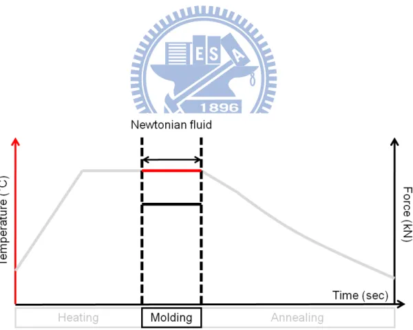
2.3.2 Molding Stage

Followed by the heating stage, the glass is molded at a fixed molding temperature (which is usually set at 30°C above At where viscosity is around 108 _Pa_∙_s_{) with a}

constant molding force in the subsequent molding stage. Figure 2.9 shows the thermal and loading history of the molding stage.

Due to low viscosity at the molding temperature, glass can be modeled as a Newtonian fluid when subjected to an applied force during the molding stage. The mathematical model of Newtonian fluid can be illustrated by

3 ( )T

σ = η ε (2.10) where σ is the effective stress, ε is the effective strain rate, and η(T) is the temperature-dependent viscosity. The corresponding viscosity at any given temperature above Tg can be calculated by fitting standard reference points with the

VFT equation (eq. (2.3)).

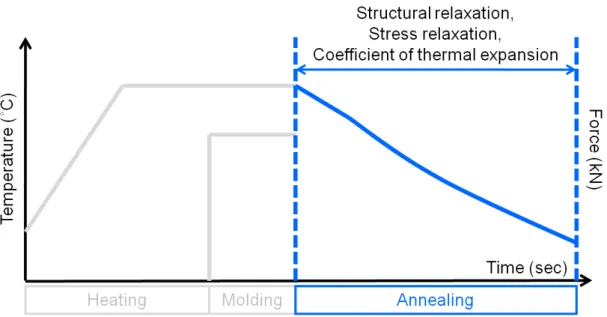
2.3.3 Annealing Stage

In the annealing stage, the applied molding force is released and the glass lens is cooled form the molding temperature. Cooling rates were controlled by the nitrogen flow rate. Figure 2.10 shows the thermal and loading history of the annealing stage. Structural relaxation, stress relaxation and coefficients of thermal expansion are the major factors governing the FE model in this stage.

In the annealing stage, because of the time-dependent characteristic of structural change in the presence of a temperature change, structural relaxation property must first be included in FEA to calculate the amount of shrinkage.

(36)

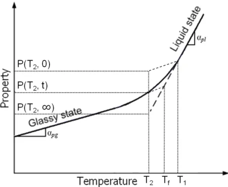
temperature, Tf, to represent the actual temperature at which a particular structure

would be fully relaxed to the liquid state (achieved equilibrium configuration) after a long time (as Figure 2.11 shows).

While glass cools through the transition region, the response to a step change in temperature from T1 to T2 can be described by [21]:

2 2 2 2 2 1 2 ( ) ( , ) ( , ) _{( )} ( ,0) ( , ) f p T t T p T t p T _{M t} p T p T T T − − ∞ ₌ ₌ − ∞ − (2.11) where 0 and ∞ respec tively represent the instantaneous and long-term values of property (p) following a temperature change. Tf is the fictive temperature, which is

defined so that the quantity on the right-hand side of the equation is the unrelaxed fraction at time t. When t=0, the structure has not yet started to relax, thus Tf (0) is T1.

As time increases, the actual temperature at which the structure has already relaxed to liquid state will become increasingly closer to T2. When the structure has sufficient

time to fully relax (t=∞), Tf(∞)=T2. The response function can then be described by

[26]:

( ) exp[ ( / ) ]

p p

M t ₌ ₋ t _τ β _(2.12)

where β is a constant between 0 and 1, and τp is the structural relaxation time.

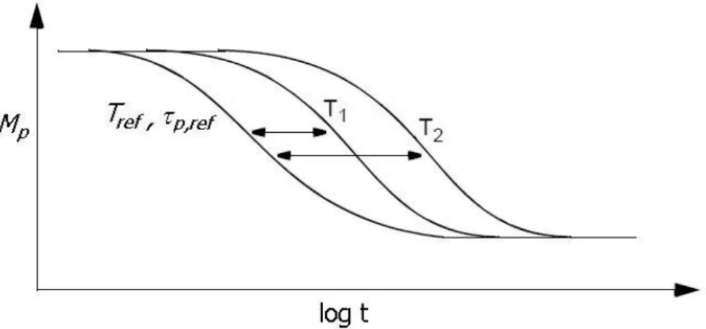
When the relaxation curves are plotted with log (time) as the abscissa, they shift toward shorter time scales without changing shape as the temperature increases (as Figure 2.12 shows). This behavior, called thermorheological simplicity, makes it possible to use relaxation times, τp,ref, evaluated at a suitable reference temperature, Tref,

and incorporate the temperature dependence in a new variable, the reduced time, ξ [26]:

, 0 ' ( ( )) t p ref _dt T t τ ξ τ = ′

∫

(2.13)

The concept of reduced time, ξ, is introduced in the spirit of thermorheological simplicity materials to capture the disparate nonlinear response curves on a single

(37)

master curve. Hence,

,

( ) exp[ ( / ) ]

p p ref

M _ξ ₌ ₋ _{ξ τ} β _(2.14)

Because the relaxation time, τP, depends not only on temperature but also on thermal

history, Narayanaswamy [27] proposed the following equation to calculate τP:

, 1 (1 ) exp p p ref ref f H x x R T T T τ τ  _∆  ₋    = _− _ − − __        (2.15)

and the fictive temperature, Tf:

0 ( ) ( ) ( ) t ( ( ) ( ) ' f p dT t T t T t M t t dt dt ξ ξ ′ ′ = − − ′

∫

(2.16) where ∆H is the activation energy, R is the ideal gas constant and x is a fraction

parameter with a value between 0 and 1.

Once the fictive temperature is known, the volume change of glass can be represented by the derivative of the property with respect to temperature [26]:

1 ( ) _{( )} _{( )} _{( )} (0) f vg vl f vg f dT dV T _T _T _T V dT α α α dT     = +_ − _ _   (2.17) where V(0) is the initial volume, αvl and αvg are the volumetric thermal contraction

coefficients of the liquid and glass respectively. In the FEA, αvl and αvg are calculated

automatically from the input of the obtained linear coefficients of thermal expansion in the liquid state and glassy states respectively. The linear thermal strain induced from the structural relaxation behavior can then be calculated in FEA by:

1 3 (0)

th V

V

ε = ∆ (2.18) Owing to the induced linear thermal strains in the annealing stage, the corresponding stresses will occur.

Because the thermal history of the glass in the annealing stage passes through the glass transition region, which is an intermediate state between liquid and solid where glass behaves as a viscoelastic material, stresses induced from thermal strains will

(38)

have the ability to relax to an extent according to the cooling rate and the unreleased stresses finally will form the residual stresses. To calculate the residual stress, stress relaxation property is also introduced into FEA in the annealing stage.

A generalized Maxwell model was used to model the stress relaxation in the glass transition region. This Maxwell model consists of a series of springs with shear modulus Gi and dashpots with viscosity ηi (as Figure 2.13 shows). The stress relaxation

modulus G(t) and the stress relaxation function ψ(t) for this parallel model can be represented by: 1 ( ) 2 n iexp( / )si i G t G w t τ = =

∑

− (2.19) 1 ( ) ( ) exp( / ) (0) n i si i G t t w t G ψ τ = = =

∑

− (2.20) At time t=0, G(0)=2G, τsi are the stress relaxation times calculated by ηi/Gi, and wi

represent the corresponding weighing factors, obtained by fitting to the stress relaxation experimental data. This stress relaxation property can be obtained from a stress relaxation experiment (will be discussed in chapter 3) and subsequently be introduced into FEA.

2.4 Summary

From the introduction on the viscosity of the glass corresponding to a wide temperature range, to the viscoelastic and structural relaxation behaviors of the glass in the glass transition region, basic understandings of the mechanical behaviors of the glass were presented in this chapter. Moreover, material models i.e. coefficient of thermal expansion, Newtonian fluid, structural and stress relaxation properties for the FE model are introduced respectively corresponding to the heating, molding and annealing stages in this chapter. The following chapter will describe the material property experiments on completing these material models.

(39)

Figure 2.1 Typical curve for viscosity as a function of temperature for a commercial soda-lime-silicate glass [19].

Figure 2.2 Standard points of L-BAL42 and the fitted viscosity curve (by VFT equation).

(40)

(41)

(a) (b)

Figure 2.4 Commonly used viscoelastic models (a) Maxwell model (b) Kevin-Voigt model.

(42)

(43)

(44)

Figure 2.8 Optical glass material properties for the FEA in the heating stage.

(45)

(46)

(47)

Figure 2.12 Relaxation curves exhibit thermorheological simplicity behavior at various temperatures (Tref >T1>T2) with a reference temperature Tref and evaluated τp,ref.

(48)

Figure 2.13 Generalized Maxwell model for modeling viscoelastic stress relaxation behavior.

(49)

CHAPTER 3 MATERIAL PROPERTY EXPERIMENTS

In order to obtain detailed optical glass material properties for constructing the FE model of the glass molding process, this study performed three kinds of material experiments. The thermal expansion coefficients, structural relaxation property and stress relaxation property were obtained by dilatometric measurement, DSC measurement and uniaxial stress relaxation experiment respectively. Detailed descriptions are presented in the following sections.

3.1 Thermal Expansion Experiment

For the expansion property, glass manufacturers usually only provide the coefficient of thermal expansion below Tg. Scholze [28] indicated that the thermal expansion

coefficient above Tg (αl) is about three times larger than that under Tg (αg) based on the

relationship between the volumetric change and the Poisson’s ratio. Chen et al. [17] and Yan et al. [24] directly introduced this simplified assumption into FEA on the glass molding process. Jain [2] preformed experiment to measure the thermal expansion coefficient of BK7 glass (Schott Co.). The measured αl is 3.77×10-5/°C which is over

four times larger than its αg (8.3×10-6/°C). Hence the simplified assumption cannot

accurately describe the expansion coefficient above Tg. Thermal expansion

experiment should be performed.

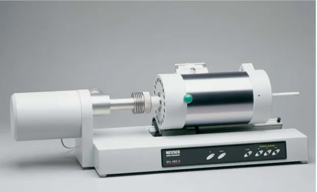
To obtain the detailed thermal expansion behavior of L-BAL42 from room temperature to molding temperature, this study performed a thermal expansion experiment using a dilatometer, Netzsch DIL 402C (Netzsch Co.), as Figure 3.1 shows. It is capable to heat the glass samples up to 1600°C. A standard cylindrical specimen with 25mm in length and 8mm in diameter was used. The experimental temperature

(50)

was controlled to be raised at a rate of 2°C/min in the low temperature range (25°C to 100°C), and 4°C/min in the high temperature range (100°C to 580°C).

Figure 3.2 shows the thermal expansion experimental results, where αg=

9.12×10-6/°C and αl =9.17×10-5/°C. The expansion curve rapidly drops when the

temperature reaches At (538°C). This is because after At, the glass continues to dilate, but it is too soft to prevent the probes at both ends of the specimen from sinking into the glass. However, the linear coefficient of thermal expansion for the liquid state can still be obtained from the maximum slope within the region between Tg and At.

The linear coefficient of thermal expansion for the solid state was obtained by linear fitting to the measured results from 100°C to 300°C. The linear coefficient of thermal expansion obtained for the glassy state differs slightly from the manufacturer-given value (8.8×10-6_{/°C). The difference may be due to slight variations in composition}

between each batch of glass. This small difference (2.8×10-7/°C) will not significantly affect the expanded quantity of the glass preform. But, owing to the lacking thermal expansion coefficient for the liquid state from the manufacturer, thermal expansion experiments should still be performed.

3.2 Structural Relaxation Experiment

Scherer [21], Webb et al, [29] and Sipp et al. [30] mentioned that the relaxation properties in volume, enthalpy, specific heat, and other material properties are equivalent with respect to structural relaxation property. Usually, volume relaxation properties are measured using dilatometer and will take hours to days to obtain the results. Moynihan et al. [31],[32] and DeBolt et al. [33] successfully obtained the structural relaxation property by using differential scanning calorimetry (DSC) to measure specific heat variation in the glass transition region with a constant heating rate and several different cooling rates. The time for one period of measurement is less

(51)

than an hour. DSC largely improves the convenience for exploring structural relaxation property of the glasses.

The DSC directly measures the heat capacity Cp (equal to dH/dT ), where H is the

enthalpy. Appendix A provides detailed descriptions on the DSC measurement. Figure 3.3 shows the schema of the temperature dependence of H and Cp during fast

and slow cooling.

According to Moynihan et al. [31], the fictive temperature is defined by:

( ) ( ) Tf '

e f _T pg

H T =H T −

∫

C dT (3.1) where He is the equilibrium enthalpy and Cpg is the heat capacity of the glass. Since

0 0 ( ) e( ) _TT p ' H T =H T −

_∫

C dT _(3.2) and 0 0 ( ) ( ) Tf ' e f e _T _pl H T =H T −

∫

C dT (3.3) Equation (3.1) can be written as:

0 ( ) ' 0( ) ' f T T p_l pg p pg T C −C dT = T C −C dT

∫

(3.4) Where Cpl is the heat capacity of the liquid (equilibrium state) and T0 is the initial

temperature, which is above the transition region. Equation (3.4) can be used to obtain

Tf (T) from the heat capacity data. Taking the derivative of eq. (3.4) with respect to T

leads to: ( ) ( ) ( ) ( ) ( ) f p pg p_l f pg f dT C T C T T dT C T C T − = − (3.5)

dTf /dT approaches unity above the glass transition (Tf =T) and zero below the

transition (Tf =Tg=constant).

According to the structural relaxation property, different thermal histories will cause different fictive temperatures Tf and different relaxation times τp. Along with the

(52)

equations proposed by Narayanaswamy [27], Hodge et al. [34] transformed these equations for numerical calculation as follows:

, , 1 , 1 ( ) ( ) f f n f n p n n n dT T T C dT T T − − − = = − (3.6) , 0 0 1 1 exp( / ) n n f n j k k k j k j T T T T q_τ β = =      = + ∆ _ −_ − ∆ __     

∑

(3.7) 0 0 , 1 (1 ) exp[ ] k k f k x H x H A RT RT τ − ∆ − ∆ = + (3.8) where Cp,n is the normalized specific heat, qk is the heating or cooling rate, β, A0, x, and

ΔH are the fitting parameters presenting different structural relaxation behavior of

different materials.

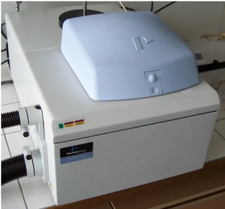
This DSC experiment was conducted using Diamond DSC (PerkinElmer Inc.), as shown in Figure 3.4. The glass sample, L-BAL42, weights 33.3mg. The measurements were taken with 4 prior cooling rates on the sample (10, 24, 60 and 100°C/min) at temperatures ranging from 600°C to 400°C and heated over the same range at 10°C/min. The specific heat variations were normalized with the difference of the measured specific heat values between 600°C and 400°C (Cp (600°C)-Cp(400°C)), and

then fitted by the above mentioned equations to obtain the fitting parameters.

Before fitting eq.(3.6) to eq.(3.8) with the DSC results, the ratio of ΔH/R can first be calculated based on the fact that viscosity obeys the Arrhenius equation (equation (2.2)). The slope of ln versus 1/T is ΔH/R, which this study calculates as 74091.33K. η

Figure 3.5 to Figure 3.8 shows the DSC results with the fitted curves. The best-fit parameters were A0=1.1×10-39, x=0.56 and β=0.69. The relaxation times τp were then

obtained and introduced into FEA at a reference temperature of 600°C, at which the equilibrium state was achieved (where dTf /dT equals 1). Table 3.1 shows the structural

(53)

3.3 Stress Relaxation Experiment

FEA on the glass molding process at the annealing stage requires the shear stress relaxation property. However, the experimental apparatus with the ability to perform shear relaxation experiment at high temperature is difficult to acquire. Fortunately, via the relationship between the uniaxial (σ11) and shear (σ12) relaxation time [21]:

11 ₂₍₁3 ₎ 12

σ σ ν

=

+ (3.9) The shear stress relaxation property can be obtained by a uniaxial compressive stress relaxation experiment.

The uniaxial compressive stress relaxation experiment was performed using a furnace embedded material testing machine, as shown in Figure 3.9. Figure 3.10 shows the settings in the furnace. The temperature is raised by heating elements bedded inside the furnace and mold sets. With maximum load of 5kN and maximum temperature to 650°C, its ability is suitable for conducting experiments on the optical glasses. Cylindrical specimen with 8mm in length and 8mm in diameter was used in this experiment.

First attempt on the compressive stress relaxation experiment was conducted at the molding temperature of 568°C (At+30°C). Figure 3.11 shows the experimental result. Obviously the stress relaxed too fast for the experimental apparatus to capture enough data points to accurately describe the relaxation curve.

Because the stress relaxation curves exhibit thermorheological simplicity behavior as well, the experiment was then performed at a lower temperature, 556°C (Tg+50°C)

to obtain a more detailed stress relaxation curve.

Figure 3.12 presents the compressive uniaxial stress relaxation results. Although the stress still relaxed quite fast at this temperature (556°C, Tg+50°C), the experimental

(54)

curve.

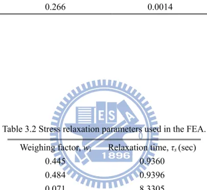
The experimental results were then fitted by a generalized Maxwell model and converted into shear relaxation properties by equation (3.9). Table 3.2 shows the weighing factors and the shear relaxation times.

3.4 Summary

The thermal expansion coefficients used in the heating and annealing stages of FEA were obtained by dilatometric measurement. Followed by DSC measurement on heat capacity, structural relaxation property was obtained from fitting the normalized measuring values with eq. (3.6) to eq. (3.8). The stress relaxation property were obtained by converting the uniaxial stress relaxation experimental results into shear ones by using eq. (3.9). These experimental obtained properties can then be inputted into FEA on the glass molding process. The verification on the FE model by experimental comparison is presented in the next chapter.

(55)

Figure 3.1 Dilatometer (DIL 402C, Netzsch) in the Center of EMO Materials and Nanotechnology, NTUT.

(56)

(57)

Figure 3.3 Enthalpy H and heat capacity Cp vs. temperature plots for a glass cooled

and then reheated through the transition region at different rates qA and qB. Higher

(58)

Figure 3.4 Differential scanning calorimeter (Diamond DSC, PerkinElmer Inc.) in the Department of Material Science and Engineering, NCTU.

(59)

Figure 3.5 DSC fitting curve (prior cooling rate: 10°C/min).

(60)

Figure 3.7 DSC fitting curve (prior cooling rate: 60°C/min).

(61)

Figure 3.9 A furnace embedded material testing machine (designed by lab member, Jung-Chung Hung and assembled by Hungta Instrument Co.)

(62)

(63)

Figure 3.11 Experimental result of stress relaxation at 568°C (At+30°C).

Figure 3.12 Experimental result of stress relaxation at 556°C (Tg+50°C) and the fitted

(64)

Table 3.1 Structural relaxation parameters used in the FEA. Reference temperature, Tref (°C) 600

Fraction parameter, x 0.56 Weighing factor, wg Relaxation time, τp (sec)

0.448 0.0164 0.286 0.0059 0.266 0.0014

Table 3.2 Stress relaxation parameters used in the FEA. Weighing factor, wi Relaxation time, τs (sec)

0.445 0.9360 0.484 0.9396 0.071 8.3305

(65)

CHAPTER 4 FEA AND VERIFICATION EXPERIMENT

Via material experiments, optical glass material properties for the FEA on the glass molding process in the heating and annealing stages were obtained. For the molding stage, because this study assumes that the optical glass behaves as Newtonian fluid, this assumption should be verified before being introduced into FEA. Therefore, in this chapter, a uniaxial compression experiment was first performed at the molding temperature and the experimental result was compared to the result obtained from FEA on the uniaxial compression with the Newtonian fluid assumption of the glass.

After these detailed optical glass material properties were all obtained, a FE model on the glass molding process was constructed. An optical glass lens molding experiment was performed to verify the feasibility of this FE model. Detailed results and discussions are presented in the rest of this chapter.

4.1 FEA Program - MARC

Marc (MSC. Software) is a commercial FEA program which is powerful to deal with nonlinear problems including geometric nonlinearities (metals bending), material nonlinearities (elastomers and metals that yield under structural or thermal loading) and boundary nonlinearities (contact problem). User subroutines and choices for Coulomb or shear friction make its usage more flexible.

Because the FEA on optical glass lens molding process includes self-defined material property (user subroutine) and glass to molds contact (contact problem with shear friction), MARC is an ideal choice for this research.

(66)

4.2 Verification on Newtonian Fluid Behavior at Molding Temperature

In the molding process, after pure thermal expansion of the glass and molds in the heating stage, the subsequent molding stage forms the basic profile of the lens. To accurately predict the lens profile, the mathematical model of the optical glass in the molding stage must represent the behavior of glass closely.

Section 2.3.2 had described that the optical glass behaves as a Newtonian fluid at the molding temperature when subjected to an applied load, and the mathematical model can be represented by eq. (2.10). To verify the accuracy of this model, a uniaxial compression experiment was performed at the molding temperature (568°C) and compared to the FEA result.

The compression test was performed in the same experimental apparatus, mentioned in section 3.3. Cylindrical specimen with 8mm in diameter and 8mm in height was used. Strain rate was held at 0.01/s, and the experiment was conducted without lubricant. Tooling steel was used for the molds.

Figure 4.1 shows the FE model for the uniaxial compression experiment. The glass specimen was modeled with 3200, four-node, axisymmetric, quadrilateral elements. Because the glass is much softer than the molds, both the upper and lower molds were set as rigid bodies in the simulation. Newtonian fluid model was introduced into FEA to describe the flow behavior of the glass specimen.

The interfacial friction between the glass and molds is described by:

m

mk

τ = (4.1) where τ is the shear stress of the interface, m is the shear factor (0<m<1), and km is the

shear strength of the glass near the interface. This study uses a shear friction factor of 1.0, which assumes complete sticking between the glass preform and the molds.

(67)

results. The FEA result is close to the result of compression test. This means the Newtonian fluid model is suitable to describe the flow behavior of the optical glass at the molding stage.

4.3 Optical Glass Lens Molding Experiment

An optical glass lens molding experiment was conducted on GMP-207HV (Toshiba Machine Co.), as shown in Figure 4.3, which is capable to set the molding temperature up to 1500°C, to apply pressing force ranging from 0.2 to 20kN and to provide vacuum or nitrogen environment. Embedded infrared lamps are used to heat the molds and the glass preform. Nitrogen gas is used to purge air from the chamber before the molding step to prevent oxidation of the mold and it is also used to control cooling rate of the mold assembly during the annealing stage. Figure 4.4 shows the schema of this apparatus.

An industrial lens design consisting of two aspherical surfaces was used in the molding experiment. Aspherical surfaces on both sides can be described by the following equation: 2 4 6 8 10 4 6 8 10 2 2 r /R z(r) = +A r +A r +A r +A r 1+ 1-(1+K)r /R (4.2)

where R is the radius of curvature, K is the conic constant, and A4, A6, A8, and A10

are the coefficients of the aspherical surfaces. Table 4.1 lists these coefficients.

The molds were made of tungsten carbide (Fujidie Co.) with Pt-Ir coating on the molding surfaces and finely ground to λ/4 (λ=632.8nm) of surface roughness to prevent surface features from imprinting onto the lens.

A glass preform with two spherical surfaces (shown in Figure 4.5) was used for the verification experiment. The thickness, radius of curvature, and diameter of the preform were designed using the optical design software, Zemax. Both the radius of curvature of

光學玻璃模造成形之有限元素分析

國

立

交

通

大

學

機 械 工 程 學 系

博 士

論

文

光學玻璃模造成形之有限元素分析

Finite Element Analysis on the Optical Glass Molding Process

研 究 生：蔡宇中

指導教授：洪景華 教授

光學玻璃模造成形之有限元素分析

Finite Element Analysis on the Optical Glass Molding Process

研 究 生：蔡宇中 Student：Yu-Chung Tsai

指導教授：洪景華 Advisor：Chinghua Hung

國 立 交 通 大 學

機 械 工 程 學 系

博 士 論 文

中華民國九十九年六月

光學玻璃模造成形之有限元素分析

研究生

: 蔡宇中 指導教授: 洪景華 教授

國立交通大學機械工程學系

摘要

FINITE ELEMENT ANALYSIS ON THE OPTICAL

GLASS MOLDING PROCESS

Student: Yu-Chung Tsai

Advisor: Prof. Chinghua Hung

Department of Mechanical Engineering

National Chiao Tung University

ABSTRACT

誌謝

TABLE OF CONTENTS

LIST OF TABLES

LIST OF FIGURES

NOMENCLATURE

ε

ε

ε

σ

σ

CHAPTER 1 INTRODUCTION

CHAPTER 2 MATERIAL MODELS OF OPTICAL

GLASSES

η

ε

ε

σ

ε

ε

ε ε

∫

( )

t

(0)

σ

=

σ

ε

σ

σ

∫

σ

ε

ε

∫

∫

∑

∑

CHAPTER 3 MATERIAL PROPERTY EXPERIMENTS

∫

∫

∫

∫

∫

∑

機械工程學系

博士

研究生：蔡宇中

指導教授：洪景華教授

研究生：蔡宇中 Student：Yu-Chung Tsai

國立交通大學

機械工程學系

博士論文

: 蔡宇中指導教授: 洪景華教授

₌

_∫