漣漪效應與區域房價動態相關之影響因素

科技部補助專題研究計畫成果報告

期末報告

漣漪效應與區域房價動態相關之影響因素

中　華　民　國　106　年　10　月　15　日

中 文 摘 要 ： 本計畫研究區域間房價的動態互動關係以及漣漪效應的可能成因 ，選擇英國為分析之樣本國家。運用Copula模型所計算的動態相關 係數分析英國倫敦地區與其他地區在過去四十年間的關係。發現地 區間的關係多發生在經濟情況較差的階段，譬如1980年代初期、 1990年代初期與2008金融海嘯時期，在樣本期間內，倫敦與各地區 房價動態相關係數並沒有結構性轉變，但卻有慢慢降低的趨勢。本 研究也運用因果關係測試(Granger causality test)，分析各區房 價動態關係是否受到人口、所得、失業率供給等因素之地區差異所 影響，發現這些經濟變數的相關性與房價相關係是有關聯的，特別 是失業率方面。

中 文 關 鍵 詞 ： 漣漪效應、價動態相關、關聯結構、房價

英 文 摘 要 ： This project focuses on the dynamic changes of the housing price correlation in the United Kingdom. We use the copula method to estimate dynamic correlation coefficients (DCC) between ten regions and London in the last four decades, showing that the DCC generally increases during the economic downturns such as the early 1980s, early 1990s, and the 2008 global crisis. Between 1976 and 2015, we do not find structural breaks of the DCC. The effect of economic interdependence on housing price correlation is found in OLS models. Using Granger causality test, we also indicate that the interaction of housing prices will

conversely affect the interaction of unemployment rate. Finally, the spillover effects of London's housing prices has been weakening to date.

科技部補助專題研究計畫成果報告

（期末報告）

漣漪效應與區域房價動態相關之影響因素

計畫類別：個別型計畫 □整合型計畫

計畫編號：MOST 105-2410-H-004 -143

執行期間：105 年 8 月 1 日至 106 年 7 月 31 日

執行機構及系所：國立政治大學財務管理系

計畫主持人： 陳明吉

計畫參與人員： 莊士玉

本計畫除繳交成果報告外，另含下列出國報告，共 _0 份：

□執行國際合作與移地研究心得報告

□出席國際學術會議心得報告

□出國參訪及考察心得報告

中 華 民 國 106 年 9 月 30 日

漣漪效應與區域房價動態相關之影響因素

Ripple Effect and Underlying Causes of Dynamic Correlation of

Regional Housing Prices

摘要 本計畫研究區域間房價的動態互動關係以及漣漪效應的可能成因，選擇英國為分 析之樣本國家。運用 Copula 模型所計算的動態相關係數分析英國倫敦地區與其 他地區在過去四十年間的關係。發現地區間的關係多發生在經濟情況較差的階段， 譬如 1980 年代初期、1990 年代初期與 2008 金融海嘯時期，在樣本期間內，倫 敦與各地區房價動態相關係數並沒有結構性轉變，但卻有慢慢降低的趨勢。本研 究也運用因果關係測試(Granger causality test)，分析各區房價動態關係是否受到 人口、所得、失業率供給等因素之地區差異所影響，發現這些經濟變數的相關性 與房價相關係是有關聯的，特別是失業率方面。

關鍵字：漣漪效應、動態相關、關聯結構、房價

ABSTRACT

This paper focuses on the dynamic changes of the housing price correlation in the United Kingdom. We use the copula method to estimate dynamic correlation coefficients (DCC) between ten regions and London in the last four decades, showing that the DCC generally increases during the economic downturns such as the early 1980s, early 1990s, and the 2008 global crisis. Between 1976 and 2015, we do not find structural breaks of the DCC. The effect of economic interdependence on housing price correlation is found in OLS models. Using Granger causality test, we also indicate that the interaction of housing prices will conversely affect the interaction of unemployment rate. Finally, the spillover effects of London’s housing prices has been weakening to date.

Keywords: Ripple effect, dynamic correlation, copula, housing prices

I. Introduction

Rising housing prices in a regional market will spread to other regions, and this

phenomenon could be called ripple effect (Giussani, 1991). Specifically, the ripple

effect is a distinct spatial pattern in the housing market. Housing prices rise first in a

city, spread to an adjoining city, and then spread further out to the next city until this

ripple reaches the borders of the country. According to the literature, U.K. might be

the best sample to understand the ripple effect. Gray (2012) uses exploratory analysis

to show that the patterns of housing prices in Britain between 1998 and 2005, which

show a diffusion process from the Southeast region to other regions, clearly indicate a

pattern of the ripple effect.

Numerous papers have discussed the possible driving forces of the interaction of

housing prices (Meen, 1999; Zhu, Füss, and Rottke, 2013; Yunus and Swanson, 2013;

Kallberg, Liu, and Pasquariello, 2014). Zhu et al. (2013) calculate economic

interdependence among 19 metropolitan areas in the U.S., showing that strong

comovement of housing prices also occurs between areas that share similar economic

conditions. Yunus and Swanson (2013) point out that the co-integrate levels of

regional per capita income and GDP are in enough to explain those levels of 9

housing markets in the U.S. Kallberg et al. (2014) decompose housing price index

into fundamental and excess return, the portion of index that cannot be attributed to

financial factors, indicating that the comovement among 14 metropolitan areas in the

U.S. mostly comes from the fundamental portion rather than excess one.

This paper discusses the interdependence of housing prices in U.K. by the

dynamic correlation between London and other ten regions from 1976Q1 to 2015Q1.

understand the driving forces of housing-price interdependence, we calculate

time-varying correlation coefficients by copula method and document the following

findings. First, the levels of housing price correlation generally are driven by

geographic connection, and the trends of housing price correlation have a negative

relationship with U.K. economy. Second, the housing price correlation between most

regions and London do not exist structural breaks during the study period. Next,

besides the geographic connection, economic interdependence also affects the housing

price correlation. Finally, the interaction of housing prices will conversely drive the

interdependence of labor market.

This paper provides the following contributions to the literature. First, Prior

literature discusses ripple effect on the basis of a static correlation, but economic

comovement should produce a wave over time rather than continue at a static level.

With dynamic correlation coefficients, we comprehensively describe the dynamic

patterns of housing price correlation from 1976 to 2015. We show that the housing

price correlations on average are higher during the economic downturns such as the

early 1980s, early 1990s, and the 2008 great recession. Consistent with Zhu et al.

(2013) and Yunus and Swanson (2013) indicating the higher interaction between

housing prices during the economic downturns in the U.S., we provide some evidence

in U.K.

Second, this is the first paper empirically testing the determinants of housing price

correlation in England. Compared to Zhu et al. (2013) and Kallberg et al. (2014) using

the weight of economic interdependence or decomposition of housing prices to

measure the effects of economic forces, we directly examine the relationship between

interdependence generally has a positive effect on the housing price correlation, while

the high correlation of population may reflect low migration activities and decrease

the housing price correlation.

Third, we test structural breaks of time-varying correlations. Compared to prior

studies showing the structural breaks of housing price correlation in Singapore and the

U.S., we do not find structural breaks from the housing price correlation between

London and ten regions in U.K. (Liao, Zhao, Lim, and Wong, 2014; Kallberg et al.,

2014). Therefore, the housing price correlation tends to be more stable in U.K.

Finally, we examine the causality relationship between housing price correlation

and economic variables. In contrast to the literature predicting a one-way causality

relationship between the economic interdependence and housing price correlation, the

results show that the interaction of housing market can conversely affect the

correlation of unemployment rate (Holmans, 1990; Meen, 1999; Zhu et al., 2013).

Our findings also provide evidence of the effect of housing prices and supply on the

labor market in an intra-region level (Saks, 2008; Sasser, 2010).

The remainder of the paper proceeds as follows. Section 2 introduces the related

literature of ripple effect. Section 3 describes the research design and data. Section 4

presents the empirical analysis. Section 5 concludes this study.

II. Related literature of ripple effect

Long-run convergence of the regional housing prices

Among the studies discussing the ripple effect, a strand of papers tests the

long-run convergence of the ripple effect (MacDonald and Taylor, 1993; Cook, 2003;

Cook, 2005; Holmes and Grimes, 2008; Gray, 2012). MacDonald and Taylor (1993)

the U.K., but they also find weak evidence in other regions. Cook (2003) uses the

asymmetric unit root tests to find the widespread convergence of housing prices in a

number of regions of the U.K., suggesting that the failure of previous analyses to

uncover convergence is due to an underlying asymmetry in the adjustment process

being ignored. Cook (2005) further shows that the reversion to the equilibrium of

regional housing prices occurs more rapidly when housing prices in the South of U.K.

decrease relative to other regions.

Different to the previous literature, Holmes and Grimes (2008) calculate the first

principal component based on regional-national housing prices differentials, showing

that the stationary of this ratio implies the convergence of regional housing prices.

Gray (2012) uses region-level data of Britain to analyze the pattern of the ripple effect,

implying that spatial spillover of housing price growth is unlikely to work on

interlocked markets suffering from obstacles to commuting and migration. In sum,

existing studies have failed to reach a consensus on whether or not regional housing

prices exhibit long-run convergence with each other (Holmes and Grimes, 2008).

Determinants of the ripple effect

Another strand of papers studies the determinants of the ripple effect, Meen

(1999) greatly reviews the prior literature and proposes four possible explanations for

the ripple effect. The first is migration; households living in a rising market might

move to an adjacent city that has relatively lower housing prices, causing the raised

prices to spread out to other cities (Giussani and Hadjimatheou, 1991; Thomas, 1993;

Alexander and Barrow, 1994). The second is equity transfer; this supposes that house

price is an indicator of equity, and the migrated purchasers bring greater buying power,

spatially limited arbitrage; arbitrageurs try to take profits from the price differential in

neighboring markets, but various costs slow the process and create a pattern of prices

similar to the ripple effect (Pollakowski and Ray, 1997). The final reason is the spatial

patterns in the determinants of housing prices. Because economic activities first arise

in one city and then spread out to others, housing price performance is a lagged

movement causing similar ripple patterns to economic activities (Holmans, 1990).

After Meen (1999), several papers discuss the reasons for the ripple effect in U.S.

Miao, Ramchander, and Simpson (2011) analyze the spatial dependence across 16

metropolitan statistical areas (MSAs) in the U.S., suggesting that both information

diffusion and population migration might be the potential sources for the dependence.

Zhu et al. (2013) highlights the importance of economic interdependence from the

results of 19 MSAs, indicating that regional interdependence during the subprime

period obviously increases. Kallberg et al. (2014) investigate the raw and excess

comovement among 14 MSAs between 1992 and 2008, showing that comovements

among housing markets are increasing and are mostly attributable to fundamental

correlations.

Ripple effect in other countries

The ripple effect in other countries is also verified in some studies. In Asia,

Chien (2010) employs the endogenous two-break LM unit test in Taiwan housing data

and shows that the ripple effect exists in each city in Taiwan except Taipei City. Lee

and Chien (2011) apply the panel seemingly unrelated regressions augmented

Dickey-Fuller test, showing the dependence of stationarity properties of housing

prices on the structure and properties of various regions in Taiwan. For instance, Lean

(2014) show evidence in Singapore indicating that foreign-liquidity shocks not only

enhance housing prices in the central region but also induce a ripple effect of prices

from the central city to the suburbs.

In North America and Africa, Gupta and Miller (2012a) apply various tools to

test the ripple effect in eight Southern California MSAs, and they find that different

specifications provide superior forecasts in the different MSAs. Gupta and Miller

(2012b) estimate the average RMSE of different models to conclude a similar result

from housing prices in Los Angeles, Las Vegas, and Phoenix. Balcilar, Beyene, Gupta,

and Seleteng (2013) analyze the ripple effect in five MSAs in South Africa. From the

results, it is apparent that ripple effects that originate in different places might result

from different sized houses.

3. Research design and Data 3.1 Empirical design

This paper employs the following steps. We first conduct the augmented

Dicky-Fuller unit root test to examine the stationarity of the housing price index

(Dicky and Fuller, 1979). Then, we apply the copula method to obtain the dynamic

correlation coefficients of housing price index between each region and London.1

After obtaining the copula coefficients, we report the descriptive statistics and trends

of these dynamic correlation coefficients, trying to paint a clearer picture of ripple

effect.2

1  _{We do not calculate the copula value between each pair of all eleven regions in U.K., because there} are total 45 time-series of copula values that could mess the results. We instead estimate the housing price correlation between each region and London to reflect the relation between regions and economic center.  

2

If the ripple effect exists in the data, we should see that the dynamic correlation coefficients first increase around the regions adjacent to London in 1998, then in the South of UK, and finally in the North and North West of UK.

We further use the copula coefficients as dependent variables and employ several

tests to amplify the literature. First, we test whether the dynamic correlation

coefficients have existed structural breaks from 1976Q3 to 2015Q1, based on the

methodology of Bai and Perron (1998). Second, we use Granger causality test to

understand whether the interaction of housing prices also conversely affect the

interaction of economic variables between regions (Granger, 1969). Finally, we test

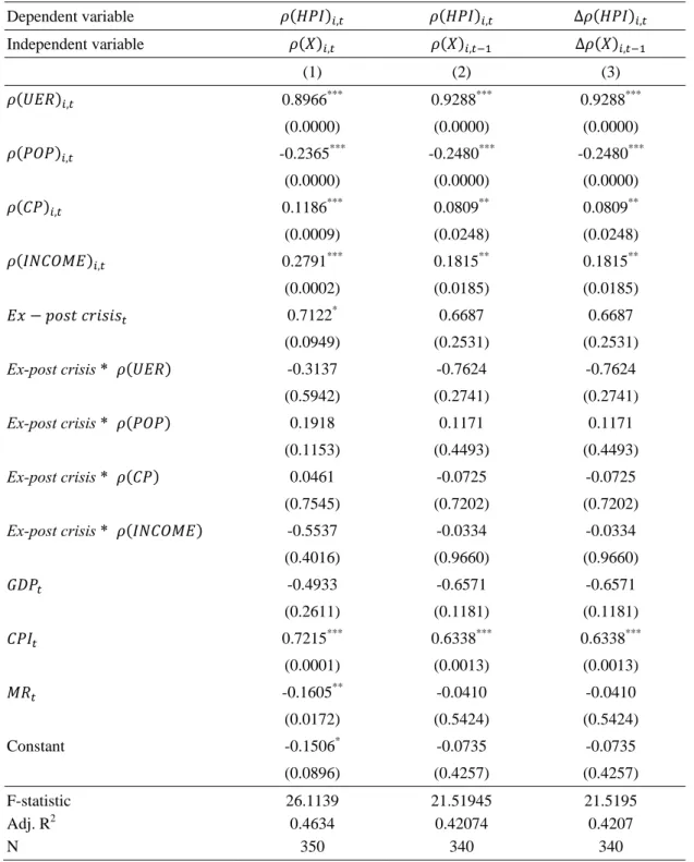
the determinants of the dynamic correlation coefficients by the following OLS model.

, , , , ,

∗ ,

, (1) where _, is the dynamic correlation coefficients between X variable of x

region and those of London; UER is unemployment rates; CP is construction permits;

INCOME is personal income; POP is regional population; GDP is gross domestic product; CPI is consumer price index; MR is fixed mortgage rates; Ex-post crisis is a

dummy variable of the after-crisis period, which equals one in year from 2009 to

2011.3 Since the dynamic correlation coefficients generally drop after the 2008 global

financial crisis, we use an indicator of after-crisis period and test whether the effects

of different driving forces drop during this period.

3.2 Methodology

This paper applies the copula method to obtain the dynamic correlation and

analyzes the trends in the correlation between regional housing prices. Sklar (1959)

indicates that any bivariate CDF (or n-dimensional distribution) can be decomposed

into two parts, the marginal distribution functions and the copula functions, the

functions describing the dependence part of the distribution. Specifically, for any        

3

The data from 1977 to 2011 is used in Granger causality test and the OLS model, because the information of construction permits is available only from 1976 to 2011.

random variables y1,t and y2,t with marginal CDFs F1(y1,t) and F2(y2,t), the values

produced by CDFs will follow a uniform distribution regardless of the functional

forms of CDFs. Thus, the following copula function C(.), which connects the two

CDFs, exists

F(y1,t,y2,t)= C(F1(y1,t), F2(y2,t)), (2)

where the copula function C(.) estimates the dependence of these two CDFs, i.e., the

function C(.) yields the joint distribution of function F(.). If the marginal CDFs are

continuous, the corresponding copula in Equation (2) is unique.

The copula is a convenient tool to integrate bivariate distributions even when the

distributions are unknown or extremely complex.4 Additionally, there is concurrently

a growing application of the time-varying copula method in housing market research,

which shows that the copula is a decent tool for modeling housing prices (Zimmer,

2012, 2015). Zimmer (2012) indicates that jointly related asset prices may exhibit

departures from normality, particularly in the tails, and he explores the housing price

connection during the financial crisis using various copula specifications. Zimmer

(2015) further employs the copula method in the multivariate GARCH model to

verify the dynamic correlations between housing prices in four U.S. cities.

The essential problem with the copula method, however, is to choose a correct

copula model that can accurately represent the dependent features of data (Coval,

Jurek, and Stafford, 2009). If an incorrect copula is chosen, the joint distribution may

be mischaracterized. To address this problem, we use Akaike information criterion

(AIC) and Bayesian information criterion (BIC) coefficients to select the better model

4

For a discussion of the literature and application of the copula-based method for economic and financial data, please refer to Patton (2006a, 2006b, 2012).

of housing data between the Gaussian copula and Student’s t copula.5 From the

results shown in Appendix A, Gaussian copula generally outperforms Student’s t

copula, we therefore use Gaussian copula in the following empirical analyses.

3.3 Data description

We use several data sources. The basic dataset used in this paper is the quarterly

seasonally adjusted National house price index from 1976Q1 to 2015Q1. We also

collect several important determinants of regional housing prices that have been

supported by prior studies. On the regional level, we obtain quarterly data such as

unemployment rates (Johnes and Hyclak, 1999; Saks, 2008), population (Mankiw and

Weil, 1989; Swan, 1995; Potepan, 1996), construction permits (Mikhed and Zemcik,

2009; Zhu et al., 2013), and personal income (Yunus and Swanson, 2013) between

1992 and 2012 from the Office for National Statistics. We further extend the sample

period up to 1976 by manually collecting the annual values of these variables from

Regional Trends magazine. In the macroeconomic level, we obtain gross domestic product (GDP) and consumer price index (CPI) from the Office for National Statistics,

and the annual effective mortgage rate (MR) is from the Bank of England.

4. Empirical results

4.1 Trends in housing prices and stationarity

Table 1 describes the distribution of housing price index for each region during

the past four decades. According to the results in Panel A, regions located in the south

such as East, South East, and South West have the highest housing prices. In contrast,

the regions located in the north including Yorkshire and The Humber, North East,

North West, and Scotland on average have the lowest housing prices compared to        

5

We follow the models shown in Patton (2006a, 2006b) and Vogiatzoglou (2010) to estimate the dynamic Gaussian and Student’s t copula.

other regions. We further apply logarithmic transformation and take the difference of

first order to estimate the growth rate of all housing price indices. As shown in Panel

B, the rank of growth rate among regions is similar to that of housing price index. The

regions with high levels of housing prices usually have a high growth rate of housing

prices.

[Insert Table 1 here]

Figure 1 further illustrates the time trends for the housing prices in each region.

Most housing price indices have similar trends between 1976 and 2015. However, the

difference in housing prices between London and other regions has been becoming

larger after 1995. In 1995, close to those of South East and South West, the housing

price index of London is 108.42. Then in 2007, after a long period with steady

economic growth rate due to the reform of employment market, the housing price

index of London is 440.50, which is much higher than the value 388.94 in South East.

This gap shrinks a little bit during the 2008 global financial crisis, but it widens again

and becomes even bigger after the recovery of the economy. In 2014, the housing

price index of London is 586.62, which is almost 1.5 times of those of South West. To

sum up, the ripple effect starting from London has been weakening to date because

the increase in London’s housing prices does not spread too much to other regions.

[Insert Figure 1 here]

To examine the stationarity of housing price indices in eleven regions, we

employ the conventional augmented Dickey-Fuller unit root test and report the results

in Table 2. After applying logarithmic transformation, all indices are stationary either

reflect the return of housing prices, we use log-differenced housing price indices to

calculate copula values, which shows the correlation of housing-price return between

regions.

[Insert Table 2 here]

4.2 Static and dynamic correlation in each region

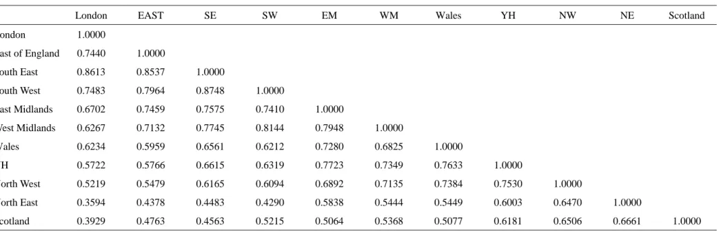
We calculate the traditional correlation between each region as a comparison

with time-varying dynamic correlation. As indicated by the results in Table 3, most

regions exhibit a higher correlation of house price indices with the regions adjacent to

them. For example, from the results in the first column, the correlation between

London and the other regions almost follows a monotonic decrease from regions in

the South to that in the North. Consistent with Gray (2012) and Gupta and Miller

(2012) showing that weak interaction between housing markets might be attributed to

weak commuting ability, the geographic connection of regions seems to be an

important driving force of the housing price correlation.

On the other hand, the correlations between regions in the Northern England are

relatively weaker than those in the other regions. The average correlation among

regions in the South such as London, South East, East of England, and South West is

0.81; the number in the Midlands such as East Midlands, West Midlands, and Wales is

0.74, while the number in the North including the other regions is 0.66. Since London

is the core of UK, the economic connection of regions in the South is relatively

stronger.

We further calculate the time-varying correlation coefficients. According to the

descriptive statistics shown in Table 4, with time-series of housing price correlation,

we can understand the distributions of housing price correlation between each region

and London during the past four decades.

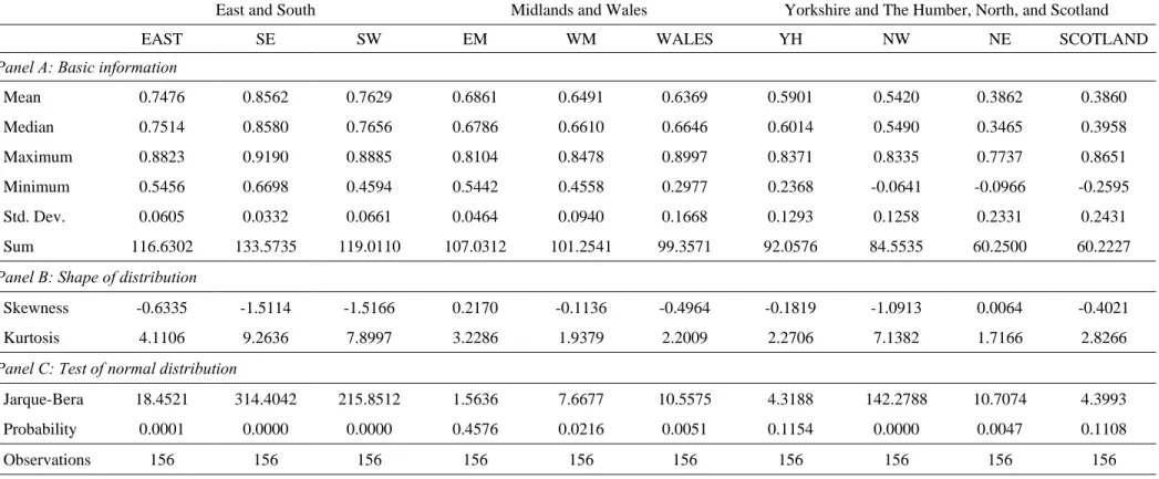
In general, the mean of correlation coefficients is similar to the static coefficients

shown in Table 3, but few characteristics help us to understand more about the

correlation between regions. First, although all regional housing markets have a

positive relationship with London’s housing market, some housing markets have had a

negative relationship in the past four decades. Second, the correlations between

London and the Northern regions are volatile. The standard deviation of these

coefficients is much higher than those in the other regions. Third, the correlation

coefficients of most housing markets have negative skewness, implying that

correlation between regions and London generally is low but substantially increases in

some period. Finally, correlation coefficients in most regions do not follow a normal

distribution, according to the results of Jarque-Bera test.

[Insert Table 4 here]

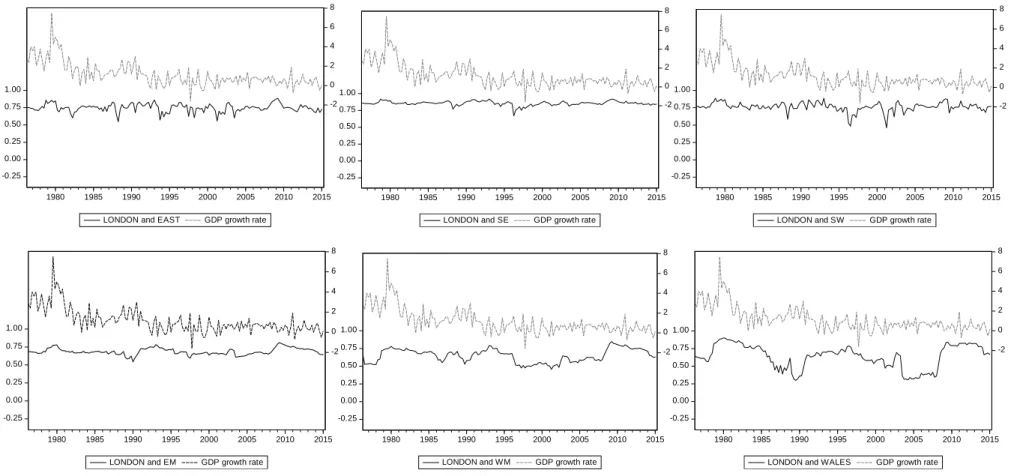
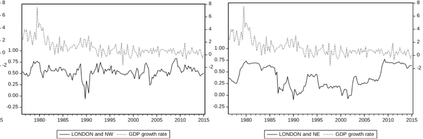
We also present the time-series of copula values in Figure 2 showing few general

tendencies of housing price correlations. First, most housing price correlations peak in

the first half of the 1980s but dramatically drop after 1985 and touch the bottom

around 1990. Next, the housing price correlations except those with North West and

Wales largely decrease around 1995 and bounce back afterward. Finally, the housing

price correlations significantly increase during the 2008 global crisis but drop

afterward. For instance, compared with other regions, the housing price correlation

correlation coefficients suddenly drop in 1982 Q1, 1988 Q1, 1993 Q4, and 2003 Q3, it

quickly rebounds thereafter.

Overall, the trends of housing price correlation are negatively related to UK

economy. According to the GDP growth rate shown as dashed line in Figure 2, few

recessions such as the early 1980s recession, the early 1990s recession, and the great

recession during the 2008 global crisis existed in the past four decades. The housing

price correlations on average decrease during the expansions and rise when the

economy falls down. On the other hand, we also find an obvious drop housing price

correlation after 2008, which is consistent with the trends shown in Figure 1.

[Insert Figure 2 here]

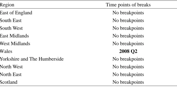
4.3 Structural breaks test of dynamic correlation coefficients

In this subsection, we address whether there are structural breaks of housing

price correlation existing from 1976 Q1 to 2015 Q1 by using the Bai-Perron

breakpoints test (Bai and Perron, 1998). Among the housing price correlation between

London and other ten regions, only the correlation with Wales exists structural break

in 2008 Q2. Before 2008 Q2, the coefficient of copula value in t-1 quarter is 0.94,

implying a relatively persistent correlation between London and Wales. Between 2008

Q2 and 2015 Q1, the coefficient of copula value in t-1 quarter becomes 0.64, showing

a change in the correlation between these two regions. To sum up, there are no

structural breaks found among the housing price correlation between London and

most regions.

4.5 Determinants of housing correlation coefficients

We next examine the determinants of housing price correlation in U.K. Different

to extant literature using comovement or cointegration analysis to test the relationship

between housing prices and economic factors, we directly examine the determinants

of dynamic correlation coefficients between regions (Zhu et al., 2013; Kallberg et al.,

2014). Specifically, we pool all the time-varying copula values of regional economic

factors between London and other regions from 1977 to 2011, and then we regress the

copula values of housing prices on those values of other economic factors.6

Table 6 reports the results containing three alternative settings of the

specification. 7 In terms of intra-region interaction, the correlations of the

unemployment rate, construction permit, and personal income have a positive relation

with the correlation between housing prices. On contrast, a higher correlation of

population will accompany with a lower interdependence of housing prices. Out

results, in general, support that the housing price correlation is likely to increase when

interdependence of economy raises up (Zhu et al., 2013; Kallberg et al., 2014).

Furthermore, since a higher correlation between populations may imply a weaker

incentive of migration activities, we find a negative relationship between the

comovement of the population and that of housing prices.

We next address the possible reason for the decrease in housing price correlation

after the 2008 global crisis. As indicated in Figure 1 and Figure 2, London’s housing

6

Because the data of regional person income is only available from 1977 to 2011 in annual level, OLS models and Granger causality test are examined by annual data during this period.

7

In column (1) of Table 6, we suppose a simultaneous relationship between the interaction of economic factors and that of housing prices. On contrast, a lead-lag relationship is assumed in column (2), which assumes that the economic interdependence leads housing price correlation. We finally employ the changes in correlations instead of levels of correlations to test how the changes in economic interdependence affect those in housing price correlation.

prices seem to spread less to other regions after the 2008 global crisis. To understand

the reasons, we test whether the effect of economic factors becomes weaker after

2008 by adding an indicator Ex-post crisis which equals one during the period 2009 to

2011 in the model. The positive coefficient of Ex-post crisis found in column (1)

shows that, other things being equal, the average housing price correlation between

2009 and 2011 is still higher than those from 1977 to 2008. However, the effect of

economic factors has no significant change after the 2008 global crisis, according to

the results of interaction variables.

To sum up, our results are in line with the findings of Zhu et al. (2013) and

Kallberg et al. (2014), showing that economic interdependence is also important to

housing price correlation. Since the data of regional construction permit and personal

income are limited to the period from 1977 to 2011, we do not find a significant

change in the effect of economic interdependence from 2009 to 2011.

[Insert Table 6 here]

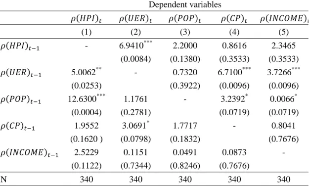
4.4 Causality relationship among housing prices and other economic factors

Finally, we test the causality relationship among regional economic factors. The

extant literature generally shows that the economic interdependence between regions

is an important force leading the housing price connection (Holmas, 1990; Meen,

1999; Zhu et al., 2013; Kallberg et al., 2014). However, the correlation of housing

prices could also conversely affect labor migration (Johnes and Hyclak, 1999; Saks,

2008; Sasser, 2010). Saks (2008) indicates that the increase in housing supply

(2010) shows that the effect of housing affordability on migration has risen during the

period 1997 through 2006 in the U.S.

With the time-series of housing price correlation, we are able to test the causality

relationship between housing prices and other economic factors. The results of

Granger causality test are shown in Table 7. Generally, the correlation of

unemployment rate granger causes the correlation of housing prices, housing supply,

and personal income. The correlation of population also leads the correlation of other

factors except for unemployment rate. On the other hand, according to the results of

column (2), we find evidence showing that the correlation of housing prices and

housing supply can conversely lead the correlation of labor market.

Consistent with Saks (2008) and Sasser (2010), we find the effect of housing

prices and supply on the labor market in an intra-region level by using the

time-varying correlation coefficients between regions. We also add to the extant

literature about the ripple effect by showing that the interaction of housing market can

conversely affect the economic connection (Holmans, 1990; Meen, 1999; Zhu et al.,

2013; Kallberg et al., 2014).

[Insert Table 7 here]

5. Conclusion

This paper explores the dynamic changes of the housing price correlation in the

United Kingdom from 1976 to 2015. Using the copula method to estimate the

time-varying correlation coefficients of housing prices between ten regions and

London, we show that the trends of housing price correlation generally are negatively

correlation between London and Wales exists structural break in 2008 Q2, while there

are no structural breaks found in other regions. With the time-series of correlation

coefficients, we also test the determinants of housing price correlation and find a

positive relationship between the economic interdependence and the housing price

correlation. Finally, the housing price correlation has two-way causality relationship

with the interaction of labor market. The housing price correlation is driven by but

also drives the correlation of unemployment rate.

The research offers insights to the literature. Compared with the extant literature

using static correlation coefficients, we calculate time-varying correlation coefficients

which provide a clearer picture of the changes in correlation (Gray, 2012). With

correlation between regions in U.K. from 1976 to 2015 containing the downturn

period up to the early 1980s, we provide a clear trend showing the negative

relationship between correlation coefficients and economy (Miao et al., 2011; Zhu et

al., 2013; Yunus and Swanson, 2013). We test the determinants of housing price

correlation and corroborate the findings using cointegration analysis (Zhu et al., 201;

Kallberg et al., 2014). We also examine the structural breaks of housing price

correlation and find that the interaction of housing market can conversely affect the

correlation of labor market (Holmas, 1990; Meen, 1999; Saks, 2008; Sasser, 2010).

Some further directions might be interesting for future research. From the trends

of housing price indices and correlation coefficients, we find that the increase in

London’s housing prices does not spread too much to other regions after the 2008

global crisis. We use an indicator to capture the period from 2009 to 2011 and test

whether the effects of economic factors on housing price correlation become weaker

of regional construction permit and personal income are limited to the period from

1977 to 2011, with a longer data, it will be interesting to understand why the ripple

Reference

Alexander, C., M. Barrow, 1994. Seasonality and co-integration of regional house prices in the UK. Urban Studies 31, 1667-1689.

Bai, J., P. Perron, 1998. Estimating and testing linear models with multiple structural changes. Econometrica 66(1), 47-78.

Balcilar, M., A. Beyene, R. Gupta, M. Seleteng, 2013. ‘Ripple’ effects in South African housing prices. Urban Studies 50(5), 876-894.

Chien, M.S., 2010. Structural breaks and the convergence of regional housing prices. Journal of Real Estate Finance and Economics 40, 77-88.

Cook, S., 2003. The convergence of regional housing prices in the UK. Urban Studies 40(11), 2285-2294.

Cook, S., 2005. Detecting long-run relationships in regional housing prices in the UK. International Review of Applied Economics 19(1), 107-118.

Coval, J., J. Jurek, E. Staord, 2009. The economics of structured Finance. Journal of Economic Perspectives 23, 3-25.

Dickey, D., W. Fuller, 1979. Distribution of the estimators for autoregressive time series with a unit root. Journal of the American Statistical Association 74, 427-431.

Granger, C.W.J., 1969. Investigating causality relations by econometric models and cross-spectral methods. Econometrica 37, 424-438.

Gray, D., 2012. Region house price movements in England and Wales 1997-2007: An exploratory spatial data analysis approach. Urban Studies 49(7), 1411-1434. Guissani, B., G. Hadjimatheou, 1991. Modelling regional house prices in the United

Kingdom. Papers in Regional Science 70, 201-219.

Gupta, R., S.M. Miller, 2012a. The time-series properties of housing prices: A case study of the Southern California market. Journal of Real Estate Finance and Economics 44, 339-361.

Gupta, R., S.M. Miller, 2012b. ‘‘Ripple effects’’ and forecasting home prices in Los Angeles, Las Vegas, and Phoenix. The Annual of Regional Science 48, 763-782.

Holmans, A., 1990. House prices: Changes through time at national and sub-national level. Government Economic Service Working Paper 110.

Holmes, M.J., A. Grimes, 2008. Is there long-run convergence among regional housing prices in the UK. Urban Studies 45(8), 1531-1544.

Johnes, G., T. Hyclak, 1999. Housing prices and regional labor markets. The Annual of Regional Science 33, 33-49.

Kallberg, J.G., C.H. Liu, P. Pasquariello, 2014. On the Price Comovement of U.S. Residential Real Estate Markets. Real Estate Economics 42(1), 71-108.

Lean, H.H., R. Smyth, 2013. Regional housing prices and the ripple effect in Malaysia. Urban Studies 50(5), 895-922.

Lee, C.C., M.S. Chien, 2011. Empirical modelling of regional housing prices and the ripple effect. Urban Studies 48(10), 2029-2047.

Liao, W.C., D. Zhao, L.P. Lim, G.K.M. Wong, 2014. Foreign liquidity to real estate market: Ripple effect and housing price dynamics. Urban Studies 52(1), 138-158.

MacDonald, R., M.P. Taylor, 1993. Regional house prices in Britain: Long-run relationships and short-run dynamics. Scottish Journal of Political Economy 40, 43-55.

Mankiw, N.G., D.N. Weil, 1989. The baby boom, the baby bust, and the housing market.

Regional Science and Urban Economics 19, 235–248.

Meen, G., 1999. Regional housing prices and the ripple effect: A new interpretation. Housing Studies 14(6), 733-753.

Miao, H., S. Ramchander, M.W. Simpson, 2011. Return and volatility in U.S. housing markets. Real Estate Economics 39, 701-741.

Mikhed, V., P. Zemcik, 2009. Do housing prices reflect fundamentals? Aggregate and panel data evidence. Journal of Housing Economics 18, 140-149.

Muellbauer, J., A. Murphy, 1991. Regional economic disparities: the role of housing. In: Bowen A, Mayhew K (eds) Reducing regional inequalities. Kogan Page, London.

Patton, A. J., 2006a. Modelling asymmetric exchange rate dependence. International Economic Review 47(2), 527-556.

Patton, A. J., 2006b. Estimation of multivariate models for time series of possibly different lengths. Journal of Applied Econometrics 21, 147-173.

Patton, A. J., 2012. A review of copula models for economic time series. Journal of Multivariate Analysis 110, 4-18.

Pollakowski, H.O., T.S. Ray, 1997. Housing price diffusion patterns at different aggregation levels: An examination of housing market efficiency. Journal of Housing Research 8, 107-124.

Potepan, M. J., 1996. Explaining intermetropolitan variation in housing prices, rents and land prices. Real Estate Economics 24, 219-245.

Saks R.E., 2008. Job creation and housing construction: Constraints on metropolitan area employment growth. Journal of Urban Economics 64, 178-195.

Sasser, A. C., 2010. Voting with their feet: Relative economic conditions and state migration patterns. Regional Science and Urban Economics 40, 122-135. Sklar, A., 1959. Fonctions de repartition a n Dimentional et Leurs Marges.

Publications de L’Institut de Statistique de L’Universite de Paris 8, 229-231. Swan, C., 1995. Demography and the demand for housing: A reinterpretation of the

Mankiw-Weil demand variable. Regional Science and Urban Economics 25, 41-58.

Thomas, A., 1993. The influence of wages and house prices on British interregional migration decisions. Applied Economics 25, 1261-1268.

Vogiatzoglou, M., 2010. Dynamic copula toolbox. Retrieved from http://www.downloadplex.com/Publishers/Manthos-Vogiatzoglou/Page-1-0-0-0-0.html.

Yunus, N., P.E. Swanson, 2013. A closer look at the U.S. housing market: Modeling relationships among regions. Real Estate Economics 41(3), 542-568.

Zhu, B., R. Füss, N.B. Rottke, 2013. Spatial linkages in returns and volatilities among U.S. regional housing markets. Real Estate Economics 41(1), 29-64.

Zimmer, D. M., 2012. The Role of Copulas in the Housing Crisis. The Review of Economics and Statistics 94(2), 607-620.

Zimmer, D. M., 2015. Time-Varying Correlation in Housing Prices. Journal of Real Estate Finance and Economics 51, 86-100.

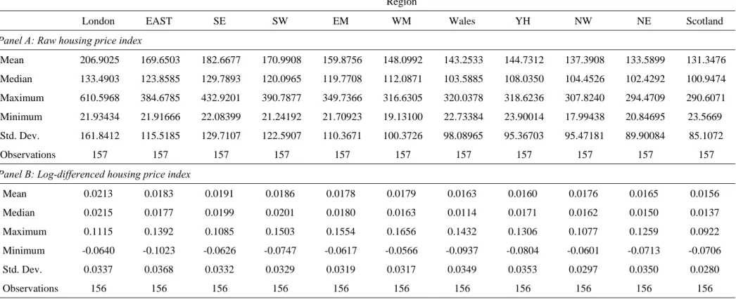
Table 1: Summary statistics of regional housing price indices

Region

London EAST SE SW EM WM Wales YH NW NE Scotland

Panel A: Raw housing price index

Mean 206.9025 169.6503 182.6677 170.9908 159.8756 148.0992 143.2533 144.7312 137.3908 133.5899 131.3476 Median 133.4903 123.8585 129.7893 120.0965 119.7708 112.0871 103.5885 108.0350 104.4526 102.4292 100.9474 Maximum 610.5968 384.6785 432.9201 390.7877 349.7366 316.6305 320.0378 318.6236 307.8240 294.4709 290.6071 Minimum 21.93434 21.91666 22.08399 21.24192 21.70923 19.13100 22.73384 23.90014 17.99438 20.84695 23.5669 Std. Dev. 161.8412 115.5185 129.7107 122.5907 110.3671 100.3726 98.08965 95.36703 95.47181 89.90084 85.1072 Observations 157 157 157 157 157 157 157 157 157 157 157

Panel B: Log-differenced housing price index

Mean 0.0213 0.0183 0.0191 0.0186 0.0178 0.0179 0.0163 0.0160 0.0176 0.0165 0.0156 Median 0.0215 0.0177 0.0199 0.0201 0.0180 0.0163 0.0114 0.0171 0.0162 0.0150 0.0137 Maximum 0.1115 0.1392 0.1085 0.1503 0.1554 0.1656 0.1432 0.1306 0.1077 0.1259 0.0922 Minimum -0.0640 -0.1023 -0.0626 -0.0747 -0.0617 -0.0566 -0.0937 -0.0804 -0.0601 -0.0713 -0.0706 Std. Dev. 0.0337 0.0368 0.0332 0.0329 0.0319 0.0317 0.0349 0.0353 0.0297 0.0350 0.0280 Observations 156 156 156 156 156 156 156 156 156 156 156 Panel A and Panel B report the summary statistics of raw housing price indices and log-differenced housing price indices from 1976Q1 TO 2015Q1, respectively. EAST is East of England; SE is South-East; SW is South-West; EM is East Midlands; WM is West Midlands; YH is Yorkshire and The Humberside; NW is North-West; and NE is North-East.

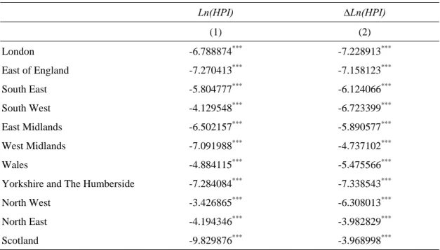
Table 2: ADF unit root tests of regional house prices indices Ln(HPI) ∆Ln(HPI) (1) (2) London -6.788874*** -7.228913*** East of England -7.270413*** -7.158123*** South East -5.804777*** -6.124066*** South West -4.129548*** -6.723399*** East Midlands -6.502157*** -5.890577*** West Midlands -7.091988*** -4.737102*** Wales -4.884115*** -5.475566*** Yorkshire and The Humberside -7.284084*** -7.338543*** North West -3.426865*** -6.308013*** North East -4.194346*** -3.982829*** Scotland -9.829876*** -3.968998***

This table reports the results of augmented Dickey-Fullers (ADF) unit root tests of all regional housing price indices (HPI). Logarithmic transformation applies to all housing price indices; First order of difference is further taken on logged housing price indices in column (2). *** stand for significance at the 1% level.

Table 3: Pearson correlation coefficients of housing price index between each region

London EAST SE SW EM WM Wales YH NW NE Scotland

London 1.0000 East of England 0.7440 1.0000 South East 0.8613 0.8537 1.0000 South West 0.7483 0.7964 0.8748 1.0000 East Midlands 0.6702 0.7459 0.7575 0.7410 1.0000 West Midlands 0.6267 0.7132 0.7745 0.8144 0.7948 1.0000 Wales 0.6234 0.5959 0.6561 0.6212 0.7280 0.6825 1.0000 YH 0.5722 0.5766 0.6615 0.6319 0.7723 0.7349 0.7633 1.0000 North West 0.5219 0.5479 0.6165 0.6094 0.6892 0.7135 0.7384 0.7530 1.0000 North East 0.3594 0.4378 0.4483 0.4290 0.5838 0.5444 0.5449 0.6003 0.6470 1.0000 Scotland 0.3929 0.4763 0.4563 0.5215 0.5064 0.5368 0.5077 0.6181 0.6506 0.6661 1.0000 This table reports the Pearson correlation coefficients of housing prices among eleven regions in U.K. EAST is East of England; SE is South-East; SW is South-West; EM is East Midlands; WM is West Midlands; YH is Yorkshire and The Humberside; NW is North-West; and NE is North-East.

Table 4:Descriptives of copula values between each region and London

Region

East and South Midlands and Wales Yorkshire and The Humber, North, and Scotland

EAST SE SW EM WM WALES YH NW NE SCOTLAND

Panel A: Basic information

Mean 0.7476 0.8562 0.7629 0.6861 0.6491 0.6369 0.5901 0.5420 0.3862 0.3860 Median 0.7514 0.8580 0.7656 0.6786 0.6610 0.6646 0.6014 0.5490 0.3465 0.3958 Maximum 0.8823 0.9190 0.8885 0.8104 0.8478 0.8997 0.8371 0.8335 0.7737 0.8651 Minimum 0.5456 0.6698 0.4594 0.5442 0.4558 0.2977 0.2368 -0.0641 -0.0966 -0.2595 Std. Dev. 0.0605 0.0332 0.0661 0.0464 0.0940 0.1668 0.1293 0.1258 0.2331 0.2431 Sum 116.6302 133.5735 119.0110 107.0312 101.2541 99.3571 92.0576 84.5535 60.2500 60.2227

Panel B: Shape of distribution

Skewness -0.6335 -1.5114 -1.5166 0.2170 -0.1136 -0.4964 -0.1819 -1.0913 0.0064 -0.4021 Kurtosis 4.1106 9.2636 7.8997 3.2286 1.9379 2.2009 2.2706 7.1382 1.7166 2.8266

Panel C: Test of normal distribution

Jarque-Bera 18.4521 314.4042 215.8512 1.5636 7.6677 10.5575 4.3188 142.2788 10.7074 4.3993 Probability 0.0001 0.0000 0.0000 0.4576 0.0216 0.0051 0.1154 0.0000 0.0047 0.1108 Observations 156 156 156 156 156 156 156 156 156 156

This table reports the summary statistics of copula values of housing prices between each region and London. EAST is East of England; SE is South-East; SW is South-West; EM is East Midlands; WM is West Midlands; YH is Yorkshire and The Humberside; NW is North-West; and NE is North-East.

Table 5:Structural breaks test of copula values between each region and London

Region Time points of breaks East of England No breakpoints

South East No breakpoints

South West No breakpoints

East Midlands No breakpoints

West Midlands No breakpoints

Wales 2008 Q2

Yorkshire and The Humberside No breakpoints

North West No breakpoints

North East No breakpoints

Scotland No breakpoints

This table reports the results of structural breaks test of copula values of housing prices between ten regions and London from 1976Q1 to 2015Q1. The Bai-Perron breakpoints test using sequential L+1 breaks vs. L is used to determine breaks (Bai and Perron, 1998).

Table 6: Determinants of housing correlation coefficients between regions Dependent variable , , ∆ , Independent variable , , ∆ , (1) (2) (3) , 0.8966*** 0.9288*** 0.9288*** (0.0000) (0.0000) (0.0000) , -0.2365*** -0.2480*** -0.2480*** (0.0000) (0.0000) (0.0000) , 0.1186*** 0.0809** 0.0809** (0.0009) (0.0248) (0.0248) , 0.2791*** 0.1815** 0.1815** (0.0002) (0.0185) (0.0185) 0.7122* 0.6687 0.6687 (0.0949) (0.2531) (0.2531) Ex-post crisis * -0.3137 -0.7624 -0.7624 (0.5942) (0.2741) (0.2741) Ex-post crisis * 0.1918 0.1171 0.1171 (0.1153) (0.4493) (0.4493) Ex-post crisis * 0.0461 -0.0725 -0.0725 (0.7545) (0.7202) (0.7202) Ex-post crisis * -0.5537 -0.0334 -0.0334 (0.4016) (0.9660) (0.9660) -0.4933 -0.6571 -0.6571 (0.2611) (0.1181) (0.1181) 0.7215*** 0.6338*** 0.6338*** (0.0001) (0.0013) (0.0013) -0.1605** -0.0410 -0.0410 (0.0172) (0.5424) (0.5424) Constant -0.1506* -0.0735 -0.0735 (0.0896) (0.4257) (0.4257) F-statistic 26.1139 21.51945 21.5195 Adj. R2 0.4634 0.42074 0.4207 N 350 340 340

This table reports the results of OLS models regressing the copula values of housing prices between ten regions and London from 1977 to 2011. is the dynamic correlation coefficients between X variable of each region and those of London; UER is unemployment rate; POP is population; CP is construction permits; INCOME is personal income; Ex-post is an indicator variable that equals to one for period from 2009 to 2011, otherwise equals to zero; GDP is gross domestic product; CPI is consumer price index; and MR is interest rate of 5-year fixed rate mortgage. P-value is reported in parentheses; ***, **, and * stand for significance at the 1%, 5%, and 10% levels, respectively. 

Table 7: Granger causality tests among copula values of regional economic factors Dependent variables (1) (2) (3) (4) (5) - 6.9410*** 2.2000 0.8616 2.3465 (0.0084) (0.1380) (0.3533) (0.3533) 5.0062** - 0.7320 6.7100*** 3.7266*** (0.0253) (0.3922) (0.0096) (0.0096) 12.6300*** 1.1761 - 3.2392* 0.0066* (0.0004) (0.2781) (0.0719) (0.0719) 1.9552 3.0691* 1.7717 - 0.8041 (0.1620 ) (0.0798) (0.1832) (0.7676) 2.5229 0.1151 0.0491 0.0873 - (0.1122) (0.7344) (0.8246) (0.7676) N 340 340 340 340 340

This table reports the results of VAR(1) Block Exogeneity Wald Tests between copula values of regional economic factors from 1977 to 2011. HPI is housing price index; UER is unemployment rate;

POP is population; CP is construction permits; and INCOME is personal income. Chi-square value is

reported, and we report p-value in parentheses. ***, **, and * stand for significance at the 1%, 5%, and 10% levels, respectively.

0 100 200 300 400 500 600 700 Q1 1976 Q1 1981 Q1 1986 Q1 1991 Q1 1996 Q1 2001 Q1 2006 Q1 2011 LONDON EAST SE SW EM W M W ALES YH NW NE SCOTLAND    

This figure presents time trends of housing price indices of eleven regions in U.K. from 1976Q1 to 2015Q1. EAST is East of England; SE is South-East; SW is South-West; EM is East Midlands; WM is West Midlands; YH is Yorkshire and The Humberside; NW is North-West; and NE is North-East.

-0.25 0.00 0.25 0.50 0.75 1.00 -2 0 2 4 6 8 1980 1985 1990 1995 2000 2005 2010 2015

LONDON and EAST GDP growth rate

-0.25 0.00 0.25 0.50 0.75 1.00 -2 0 2 4 6 8 1980 1985 1990 1995 2000 2005 2010 2015

LONDON and SE GDP growth rate

-0.25 0.00 0.25 0.50 0.75 1.00 -2 0 2 4 6 8 1980 1985 1990 1995 2000 2005 2010 2015

LONDON and SW GDP growth rate  

-0.25 0.00 0.25 0.50 0.75 1.00 -2 0 2 4 6 8 1980 1985 1990 1995 2000 2005 2010 2015

LONDON and EM GDP growth rate

-0.25 0.00 0.25 0.50 0.75 1.00 -2 0 2 4 6 8 1980 1985 1990 1995 2000 2005 2010 2015

LONDON and WM GDP growth rate

-0.25 0.00 0.25 0.50 0.75 1.00 -2 0 2 4 6 8 1980 1985 1990 1995 2000 2005 2010 2015

LONDON and WALES GDP growth rate

This figure presents time-series of copula values between ten regions and London from 1976Q1 to 2015Q1. GDP growth rate is marked by dashed line as a comparison. EAST is East of England; SE is South-East; SW is South-West; EM is East Midlands; WM is West Midlands; YH is Yorkshire and The Humberside; NW is North-West; and NE is North-East.

-0.25 0.00 0.25 0.50 0.75 1.00 -2 0 2 4 6 8 1980 1985 1990 1995 2000 2005 2010 2015

LONDOn and YH GDP growth rate

-0.25 0.00 0.25 0.50 0.75 1.00 -2 0 2 4 6 8 1980 1985 1990 1995 2000 2005 2010 2015

LONDON and NW GDP growth rate

-0.25 0.00 0.25 0.50 0.75 1.00 -2 0 2 4 6 8 1980 1985 1990 1995 2000 2005 2010 2015

LONDON and NE GDP growth rate  

-0.25 0.00 0.25 0.50 0.75 1.00 -2 0 2 4 6 8 1980 1985 1990 1995 2000 2005 2010 2015 LONDON and SCOTLAND

GDP growth rate  

Appendix A: AIC and BIC for copula values between each region and London

Gaussian copula Student’s T copula AIC BIC AIC BIC

LON_EAST -1.31E+02 -1.25E+02 -129.2154 -120.0658

LON_SE -207.6968 -201.5971 -209.8900 -200.7404 LON_SW -142.1756 -136.0761 -140.1635 -131.0139 LON_EM -97.1019 -91.0022 -103.6303 -94.4808 LON_WM -87.3424 -81.2427 -85.67933 -76.5298 LON_WALES -91.7208 -85.6211 -91.2232 -82.0736 LON_YH -66.3574 -60.2577 -71.5368 -62.3872 LON_NW -64.0329 -57.9332 -64.1308 -54.9813 LON_NE -28.3440 -22.2443 -26.8952 -17.7457 LON_SCOTLAND -38.4331 -32.3334 -36.4193 -27.2697

This appendix reports the results of AIC and BIC test for Gaussian and Student’s T copula values between each region and London from 1976Q1 to 2015Q1. LON_EAST is the copula values between London and East of England; LON_SE is the copula values between London and South-East; LON_SW is the copula values between London and South-West; LON_EM is the copula values between London and East Midlands; LON_WM is the copula values between London and West Midlands; LON_YH is the copula values between London and Yorkshire and The Humberside; LON_NW is the copula values between London and North-West; and LON_NE is the copula values between London and North-East.

Appendix B: Sensitivity of settings for testing the determinants of housing correlation coefficients between regions

Dependent variable ∆ , , Independent variable ∆ , ∆ , (1) (2) , 0.5586*** -0.0190 (0.0000) (0.8308) , 0.0619*** 0.0178 (0.0000) (0.3528) , 0.0006** 0.0014 (0.0248) (0.1167) , 0.1350** -0.0030 (0.0185) (0.4423) 0.2347 0.1494*** (0.2531) (0.0010) Ex-post crisis * -0.2643 0.3344 (0.2741) (0.7490) Ex-post crisis * 0.6605 -0.2127 (0.4493) (0.7961) Ex-post crisis * -0.0056 -0.0033 (0.7202) (0.7944) Ex-post crisis * 0.2103 -0.0056 (0.9660) (0.9298) -0.0032 0.0022 (0.1181) (0.6753) 0.1292*** 0.0000 (0.0013) (0.9990) 0.0046 0.0008 (0.5424) (0.2590) Constant -0.2250 0.6064*** (0.4257) (0.0000) F-statistic 0.05578 1.9843 Adj. R2 -0.0345 0.0337 N 340 340

This appendix reports the results of OLS model regressing the copula values of housing prices between ten regions and London from 1977 to 2011. is the dynamic correlation coefficients between X variable of each region and those of London; UER is unemployment rate; POP is population; CP is construction permits; INCOME is personal income; Ex-post is an indicator variable that equals to one for period from 2009 to 2011, otherwise equals to zero; GDP is gross domestic product; CPI is consumer price index; and MR is interest rate of 5-year fixed rate mortgage. P-value is reported in parentheses; ***, **, and * stand for significance at the 1%, 5%, and 10% levels, respectively.

105年度專題研究計畫成果彙整表

研討會論文 1 2017 Annual Conference of Asian Real Estate Society

專書 0 本 專書論文 0 章 技術報告 0 篇 其他 0 篇 智慧財產權 及成果 專利權 發明專利 申請中 0 件 已獲得 0 新型/設計專利 0 商標權 0 營業秘密 0 積體電路電路布局權 0 著作權 0

其他 0 技術移轉 件數 0 件 收入 0 千元 參 與 計 畫 人 力 本國籍 大專生 0 人次 碩士生 0 博士生 0 博士後研究員 0 專任助理 0 非本國籍 大專生 0 碩士生 0 博士生 0 博士後研究員 0 專任助理 0 其他成果 （無法以量化表達之成果如辦理學術活動 、獲得獎項、重要國際合作、研究成果國 際影響力及其他協助產業技術發展之具體 效益事項等，請以文字敘述填列。）　　

科技部補助專題研究計畫成果自評表

請就研究內容與原計畫相符程度、達成預期目標情況、研究成果之學術或應用價

值（簡要敘述成果所代表之意義、價值、影響或進一步發展之可能性）、是否適

合在學術期刊發表或申請專利、主要發現（簡要敘述成果是否具有政策應用參考

價值及具影響公共利益之重大發現）或其他有關價值等，作一綜合評估。

1. 請就研究內容與原計畫相符程度、達成預期目標情況作一綜合評估

■達成目標

□未達成目標（請說明，以100字為限）

　　□實驗失敗

　　□因故實驗中斷

　　□其他原因

說明：

2. 研究成果在學術期刊發表或申請專利等情形（請於其他欄註明專利及技轉之證

號、合約、申請及洽談等詳細資訊）

論文：■已發表　□未發表之文稿　□撰寫中　□無

專利：□已獲得　□申請中　■無

技轉：□已技轉　□洽談中　■無

其他：（以200字為限）

本研究完成計畫，達成目標，已發表在2017 Asian Real Estate Society

Annual Conference，但未來仍會繼續深入，在發表過程中仍會進行修正，以

更提升最終研究計畫品質

3. 請依學術成就、技術創新、社會影響等方面，評估研究成果之學術或應用價值

（簡要敘述成果所代表之意義、價值、影響或進一步發展之可能性，以500字

為限）

區域間不動產市場會存有連動波及關係，此連動波及關係的範圍與強弱是學術

界與政府都關心的議題，此連動波及的範圍與強弱也會隨時間變化，特別是台

灣區域均衡雖是政府之政策目標，但這些年來區域發展不均日趨嚴重，造成房

市也朝向不均衡方向發展，區域間房價之間的連動關係也因此在變化之中，本

研究由於需要較長的時間樣本，採用英國為分析標的，而英國與台灣同樣為較

小國家，同為有一個核心城市，故英國研究會有參考價值，特別對台灣投資者

、建商與政府對不動產市場做決策有很大參考價值，此為本計劃貢獻之處。

4. 主要發現

本研究具有政策應用參考價值：□否　■是，建議提供機關內政部,經濟部,財

政部,

（勾選「是」者，請列舉建議可提供施政參考之業務主管機關）

本研究具影響公共利益之重大發現：■否　□是　

說明：（以150字為限）