A Dynamic Object Tracking Protocol for Wireless Sensor Networks

全文

(1)A Dynamic Object Tracking Protocol for Wireless Sensor Networks* Tzung-Shi Chen Wen-Hwa Liao Abstract In this paper, we propose a protocol for dynamically tracking a mobile object in a sensor network. The problem we discussed here is that one source object is set to track a mobile object, called target, in a wireless sensor network. The source is moving to approach the target. In this kind of object tracking sensor networks, the activated sensor nodes can detect an object to be tracked as well as to keep tracking of information for the source. The source follows the movement route to approach the sensor node which the object is covered in. In order to maintain the accurate route, the sensors can be worked together to dynamically adjust the route between the target and source. The source will move to reach the site of the object quickly along the adjusted route in a power saving way. Finally, we compare our scheme with others with flooding-based mechanism. Index Terms—Mobile computing, object tracking, routing, spatiotemporal guarantee, wireless sensor networks.. I. INTRODUCTION. R. ecent advances in wireless communications and electronics have enabled the development of low-cost, low-power, multifunctional sensor nodes that are small in size and communicate un-tethered in short distances. These tiny sensor nodes, which consist of sensing, data processing, and communicating components, leverage the idea of sensor networks. A wireless sensor network (WSN) is composed of a large number of sensor nodes that are densely deployed either inside the phenomenon or very close to it. One of the most important areas where the advantages of sensor networks can be exploited is for tracking mobile object. Scenarios where such network * This research is supported by the National Science Council of the Republic of China, Taiwan, under Contract Nos. NSC 94-2213-E-024 -002 and NSC 94-2213-E-036-012. T.-S. Chen is with Department of Information and Learning Technology, National University of Tainan, Tainan 700, Taiwan (e-mail: [email protected]) W.-H. Liao is with Department of Information Management, Tatung University, Taipei 104, Taiwan (e-mail: [email protected]) M.-D. Huang is with Department of information management, Chang Jung Christian University, Tainan 700, Taiwan. H.-W. Tsai is with Department of Computer Science and Information Engineering, National Cheng-Kung University, Tainan 700, Taiwan.. Ming-De Huang Hua-Wen Tsai may be deployed can be both military (tracking enemy vehicles, detecting illegal border crossings) and civilian (tracking the movement of wild animals in wildlife protection). Typically, for accuracy, two or more sensors are simultaneously required for tracking a single object, leading to coordination issues. Additionally, given the requirements to minimize the power consumption due to communication or other factors, we would like to select the fewest essential number of sensors dedicated for the task while all other sensors should preferably be in the hibernation or off state. Because it involves a large amount of cooperation among sensors, object tracking sensor network provides significant research opportunities in terms of energy management. In order to simultaneously satisfy the requirements like power saving and improving overall efficiency, we need large scale coordination and other management operations. In object tracking sensor networks, we assume that the sensors of WSN are active. But this assumption causes the energy to consume too much. This is because that too much sensors detect the object and transmit the data at the same time. Hence, it can make use of Collaborative Signal and Information Processing (CSIP) to reduce the energy consumption. CSIP have been proposed in [1][6][14][20]. In general, the object tracking of protocols are classified into cluster-based and non-cluster-based protocols in sensor networks. In cluster-based protocols [4][5][15][19], when a non-cluster sensor nodes detected an object, it forwards the information to the nearest cluster head. And then the cluster head collects and forwards the information to the sink. This approach reduces the energy consumption and the required communication bandwidth, but it prolongs the lifetime of the wireless sensor network. In non-cluster-based protocols, no any cluster heads exist in the sensor network. When a sensor detects an object, it records the object information in its memory. A user queries the sensors in WSN while the information of tracked object is needed. The sensor that it has the information of the tracked object replies the information to the user. Kung et al. [11] and Lin et al. [13] assume that a logical structure to connect sensors exists in a sensor network. They build the hierarchical structure that allows the system to handle a large number of tracked objects. In addition, Tseng et al..

(2) [16] proposed a novel protocol based on the mobile agent. Once a new object is detected, a mobile agent will be initiated to track the roaming path of the object. The mobile agent will choose and stay the sensor that is the most close to the tracked object. The agent invites some nearby slave sensors to track the position of object cooperatively and inhibits other irrelevant sensors to track the object. The overhead of communication and the sense energy are reduced. In order to reduce the energy consumption, the prediction-based methods [7] [18] [19] are used to predict the location of the movement object. When a sensor detects an object, it forwards the information of object to its cluster head. The information contains the location of object, the velocity of object, and the move direction of object. The cluster head calculates and predicts the location of object and it wakes up the sensors close to the object in order to do the sensing task. When an active sensor predicts the next location of object, it must wake up the sleeping sensors before the object enters in their sensing region. It is called spatial and temporal delivery guarantee. The spatiotemporal delivery guarantee is to wake up all the nodes at time t in forwarding zone Z. Some literatures [3][8][9] have been discussed for spatial and temporal delivery guarantee. When a sensor wants to forward the information of object to the sink or its cluster head, a routing protocol is used. The greedy forwarding is the basic method. The next forwarding hop is chosen the minimum distance from the sender to the destination. However, the greedy forwarding is failed while the sensors have exhausted energy, in the voids of space or the route is a dead-end. This makes that the object information is unable to reach the sink or the cluster head. It is called the holes problem. In this paper, we propose a novel object tracking protocol in sensor networks. We can accurately track the mobile object and save the power consumption of sensor nodes to prolong lifetime of a wireless sensor network. A source is set to track a mobile object called target. The activated sensor nodes can detect a tracked object and keep the information of track for the source. The source follows the tracking route to approach the sensor node that covers the tracked object. In order to maintain the accurate route, the sensors can cooperate to adjust the route between the target and the source dynamically. For accurately tracking the object, we consider the holes problem and the spatiotemporal guarantee in this paper. Furthermore, we also consider the move speed and the direction of the tracked target. The source would reach the site of the object along the adjusted route faster than along the tracking route. For dynamical tracking object, our protocol can save more energy of battery than other flooding based protocols. Therefore, we can extend the lifetime of the entire. wireless sensor network. The rest of this paper is organized as follows. The problem definition and protocol overview is discussed in Section II. In Section III, we present our tracking object protocol in wireless sensor networks. We compare out proposed protocol with three flooding-based protocols in Section IV. The conclusions from this work are presented in Section V.. II. PRELIMINARY In this section, we introduce the problem definition and protocol overview. We describe the environment of the sensor network in problem definition. And then an example is illustrated in protocol overview. A. Problem Definition In our protocol, a mobile user, called source object, wants to track a mobile object, called target, in a wireless sensor network. In order to provide correct routing in the presence of dead-end, the face routing [10] [12] has been integrated in our proposed protocol. Here we have several assumptions of our proposed protocol listed in below. The sensor nodes have two states, active and sleep. When a sensor is in active state, it can sense object, receive or transmit data any time. When a sensor is in sleep state, it stops to sense, receive or transmit. But it would wake up at a predefined period. If it receives a wakeup packet, its state will be changed as active. And then its state is sustained in active state until the active time expires. A sensor knows the accurate location of object, because of the object could transmit its location to the sensors or the sensor utilizes triangle calculation to know the location of object. The triangle calculation has been proposed in [2]. Each node knows its location and this information can be acquired from global positioning system (GPS) or other mechanisms. L(o) denotes the location of object o. The communication and sense range for each node are both same. For preventing to lose the tracking object and the holes problem, we use a spatial neighborhood to detect the mobile object. We used the face-aware routing strategy [9] to build the spatial neighborhood. Here, a set of nodes in its spatial neighborhood is called neighboring face nodes. Some notations are given below. Fi is denoted as the identity of face i in the network. (X, Y) is denoted the connection (edge) between two sensors X and Y. We assume that the mode of faces is established in the sensor network. A node uses a discovery message to seek out its neighboring face nodes. We use the counterclockwise to seek out the interior of a closed polygonal region (a face). After a face discovery message seeks a face, it collects the location of all nodes on the face. And then a message is forwarded to inform the nodes in this face of the complete discovery results. So each node knows.

(3) the location of nodes in the same face. B. Protocol Overview We illustrate the overview of our object tracking in Fig. 1. A scenario is that a source S wants to chase a mobile target. It employs the sensors to get the location of the target. But we can not predict the tracks of mobile target. If the source uses continually a flooding method for chasing the location of target, the energy of sensors would be totally consumed soon. We propose a protocol which can not only save the energy of sensor but also chase the tracks of target accurately. First, the source uses the flooding method to get the location of target. E.g. the source S knows that the present location of target is near sensor n1. But the target will move at any time. Then, the sensors begin to record the track of target. We utilize a face structure to distinguish different areas in sensor network. A sensor n detects that it has come in this face when the target enters another face. This sensor is named ingress node. Therefore, the track of target will be recorded in a set of ingress nodes when it moves. E.g. the track of target is recorded as <n1, n2, n3, n4, n5, n6 >. The source will chase the target along the track. This is similar to that ants (sensors) release a substance called pheromone to communicate with other ants (the source S). The other ants (the source S) will follow the scent and reach to a food source (the target).. Fig. 1: An overview for the object tracking.. III. MOVEMENT OBJECT TRACKING In this section, we introduce the detail of proposed protocol. We focus on communication cost, communication distance, the number of sensors that must transmit information to sink, holes problem and spatiotemporal guarantee while we design the proposed object tracking protocol. And we consider a mobile user to track a mobile object in a sensor network. A. Target Discovery In this subsection, we discuss the process of target discovery. A source S wants to track a target o but it. does not know the location of target o. The source S employs the sensor network to discover the target o. It issues a query packet and uses flooding method to seek the target. If a sensor n knows the target o in its sense range and it is the closest to the target o than others, it forwards a reply packet to the source S. Because every node knows its entire face neighboring node’s location, it can check whether it is the closest to the target or not. The format of query packet is query(packet type, source id, target id, sequence number), which the packet type is QUERY, the sequence number is used to avoid forwarding the duplicate packet. The format of reply packet is reply(packet type, source id, target id, the location of the object), which the packet type is REPLY. This process is similar to the route discovery process in ad hoc networks. When the sensor n issues the reply to the source, it sets its state and the active time as active and infinity, respectively. It also acts an ingress node and begins to track the target. The first ingress also is a checkpoint named checkface (discussed in Section 3.D). B. Detecting the Mobile Target When a sensor receives a request packet and it is the closest to the target o, this sensor acts as an ingress node to track the target. If it does the detecting by itself, it may lose the track of target while the target has moved. For tracking the target accurately, this ingress node informs its neighboring face nodes to cooperate tracking target. When a node n asks its neighboring face nodes to wakeup and to detect the target o, it forwards a wakeup packet to inform them. Let Y is a set of the neighboring face nodes of n, and Y1 , Y2 , K , Yk be all neighboring face nodes of n. The wakeup packet format is wakeup(packet type, ingress id, sender id, face id, the location of target, active time, face hop count), which the packet type is WAKEUP, the face hop count indicates that how many distances the target has already moved. The face hop count is set as 1 initially. After all of neighboring face node receive the wakeup packet, they are in active state and do the target detecting. The ingress node forwards the wakeup packet periodically if it still is the closest to the target. If the target is far away from the ingress node, a sensor Yi ( i ∈ Y ) will detect the target and it is the closest to the target o. Because every node has the information of its neighboring face nodes, it can check whether he is closest to the target. The ingress node stops to forward the wakeup packet, but the sensor Yi will forward a wakeup packet to its neighboring face nodes. In other words, every active node detects the target and checks whether it is closest to the target. We define that a sensor that is the closest to the target can forward the wakeup packet, but the others can not. The information of target is stored in all of neighboring.

(4) face nodes until the active time expires. And then the sensor enters the sleep state. The wakeup packet can wake up the sleep sensors or refresh their active time. The active time of ingress node is infinity. This is because it must go to guide the source S to chase the mobile target o. Therefore, it must be in active state until the source S comes in. An example for detecting the mobile target is illustrated in Fig. 2. Now, a mobile target is in face F1 at T. Three sensors n1, n2 and n3 can detect the target. When n1 receives a query packet and it is the closest to the target than n2 and n3, it replies a reply packet to the source and it acts as an ingress node. It will forward a wakeup packet to its all neighboring face nodes and wake up them. n1 forwards three wakeup packets (WAKEUP, n1, n1, F1, L(o), t, 1), (WAKEUP, n1, n1, F2, L(o), t, 1) and (WAKEUP, n1, n1, F3, L(o), t, 1) to face F1, F2 and F3, respectively. These nodes include n2, n3, n4, n5, n6 in F1, n9, n2 in F2 and n6, n7, n8, n9 in F3. The target may have moved to the neighbor face at next period (T+1). E.g. the target may move to the face F2, F3, F4, F5 or F6 in Fig. 2 (a).. target), and then it will chase the mobile target. The face hop count is increased when the target moves into a new face. C. Tracking Target When a target o is tracked by a source S, the sensors must record the tracks of mobile target. A source S knows the location of target/first ingress node after a target discovery process, and then it begins to move towards the location of first ingress node (checkface). When it reaches the location, the first ingress sensor informs it about whether the target is still in here or not. If yes, the source S catches the target o. If no, the sensor informs the source the location of next ingress node. Then, the source moves towards the location of next ingress node again. The first ingress node also informs the next ingress node the source will arrive in your location. The next ingress becomes the first ingress node (checkface). This process is repeated until the source catches the target. The source will pursue the target along the ingress nodes. An example for tracking target is shown in Fig. 3. The source S follows the path of ingress nodes <n1, n2, n3, n4, …> named face tracks to pursue the target o. After the ingress node informs the source about the information of target, it sets its active time and state as 0 and sleep, respectively. It does not track the target for the source S anymore.. Fig. 2: An example for detecting mobile target. If the target wants to go to the neighbor face F4, it must cross an edge (n5, n6). When the target moves to the neighborhood of n5 and it still is in face F1, it forwards three wakeup packets (WAKEUP, n1, n5, F1, L(o), t, 1), (WAKEUP, n1, n5, F4, L(o), t, 1) and (WAKEUP, n1, n5, F5, L(o), t, 1) to face F1, F4 and F5, respectively. When the active time of n8 and n9 are expired, the sensors n8 and n9 change their state as sleep shown in Fig. 2(b). If the target enters F4 at T+1 and n5 also is the closest to the target than others as shown in Fig. 2(b), n5 forwards three wakeup packets (WAKEUP, n5, n5, F1, L(o), t, 2), (WAKEUP, n5, n5, F4, L(o), t, 2) and (WAKEUP, n5, n5, F5, L(o), t, 2) to its all neighboring face nodes and wake up them. These nodes include n6, n1, n2, n3, n4 in F1, n10, n11, n12, n7, n6 in F4 and n4, n10 in F5. New, n5 is the ingress node of face F4 and the face hop count is set as 2. n1 records n5 as the next face ingress node. When the source comes in the range of n1, n1 guides the source to n5. The source follows a sequential ingress nodes (the track of. Fig. 3: An example for tracking mobile target. D. Adjusting Face Tracks In this subsection, we discuss that how to adjust the face tracks. When the velocity of the mobile target is faster than the one of source, it is very difficult for the source to chase the mobile target. The face tracks maybe are not the optimal tracks. Therefore, we adjust the face tracks to make that the source can chase the target faster. The face tracks needs to adjust when the face hop count has already been accumulated to K hops. The Kth ingress node is set as checkface. An overview for adjusting face tracks is shown in Fig. 4. Fig. 4 (a) shows that the target o has passed faces F9, F6, F4, F5, F8 and F10. The face tracks are <n1, n2, n3, n4, n5>. This face tracks are not the optimal tracks. Here assumes that the value K is 5 and n1 is the checkface (first ingress node). When the target has passed 5 faces from last checkface, the 6th ingress node.

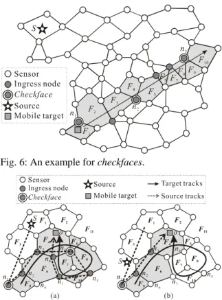
(5) (n5) begins the adjusting face tracks process. This is because that the 4th and 5th ingress nodes are same (n4). After adjusting face tracks, the optimal face tracks <n1, n6, n7> are shown in Fig. 4 (b). The optimal face tracks are the shortest path computed from the last checkface to Kth ingress node.. Fig. 4: An overview for adjusting face tracks. When a target o enters to the Kth face from last checkface, the Kth ingress node forwards an infoadj packet to the last checkface. The infoadj packet format is infoadj(packet type, the Kth face id, the Kth ingress id, the location of Kth ingress node, the face hop count Kth ingress node, the preceding ingress node id), which the packet type is INFOADJ. This packet includes the information of the Kth ingress node and it is forwarded to the last checkface. When an ingress node between the last checkpoint and the Kth ingress node receives this packet, it is not an ingress node anymore. The ingress nodes between the last checkpoint and the Kth ingress node are canceled. When the last checkface receives this infoadj packet, it computes the shortest path from its location to the location of Kth ingress node and it finds a node n that is the closest to the Kth ingress node in its faces. The node n is the new next ingress node. The checkface forwards an adjustment packet to the next ingress node n. The adjustment packet format is adjustment (packet type, the ingress node id, the original Kth ingress node id, the new next ingress node id, the face hop count), which the packet type is ADJUSTMENT. The face hop count of node n is set as the face hop count of last checkface added 1. And then the node n also uses the same process to find the next ingress node. This process is repeated until a node in the Kth face receives the adjustment packet.. An example for adjusting face tracks is shown in Fig. 5. We assume that K is set as 5, n1 is a checkface (the first ingress node) and n5 is the Kth ingress node in face F10. In Fig. 5 (a), n5 forwards an infoadj packet to the last checkface (n1). Then, n2, n3 and n4 cancel the ingress nodes of them. When the last checkface (n1) receives the infoadj packet, it computes the shortest path to n5 and the new next ingress node is n6. The node n7 is a node in face F10, so the new set of ingress nodes is <n1, n6, n7>. If the face hop count of n1 is 1, the face hop count of n6 and n7 are 2 and 3, respectively. If the face hop count of new ingress node in the original Kth face also is K, this new ingress node is set as a checkface. An example is illustrated in Fig. 6. The movement path of the mobile target is a straight line. So the face tracks is the optimal tracks and the sequence of faces are <F1, F2, F3, F4, F5, F6, F7, F8, F9, F10>. Here assume that the value of K is set as 4. Therefore, there are three checkfaces n1, n2 and n3 in the face tracks.. Fig. 6: An example for checkfaces.. Fig. 7: An example for adjusting loop face tracks.. Fig. 5: An example for adjusting face tracks.. E. Adjusting Loop Face Tracks This subsection discusses the loop face tracks problem. When the face tracks forms a loop, we must to delete the loop tracks. An example for adjusting loop face tracks is illustrated in Fig. 7. Here assumes that the face tracks are <n1, n2, n3, n4, n5, n7, n8>, the sequence of faces are <F9, F6, F4, F5, F8, F10, F7, F4>, n1 and n4 are the checkfaces. In Fig. 7 (a), the faces loop is <F4, F5, F8, F10, F7, F4>. When the mobile target o enters to the face F4, the ingress node is n8 and.

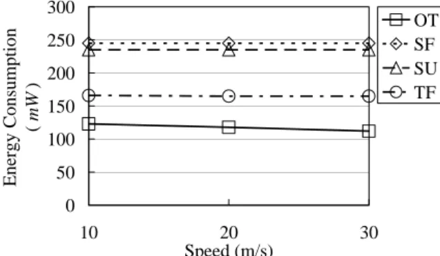
(6) In this section, our proposed dynamic tracking object protocol is compared with the flooding-based dynamic tracking protocols. The experiments are implemented in NS2 simulator [17]. A. Protocols Based on Flooding We compare our proposed protocol with three tracking object protocols based on flooding. Three tracking object protocols based on flooding are Threshold Flooding (named TF), Schedule Flooding (named SF), and Schedule Updating (named SU). Our proposed protocol is called dynamically object tracking (named OT). In TF protocol, the target discovery is similar to our protocol. When the source gets the location of mobile target, it moves towards the location. When it reaches the location, the target discovery process is executed again. The procedure is repeated until the source catches the mobile target. In SF protocol, the source executes the target discovery process with a predefined period. The time interval is set as 2 second in the simulation. In SU protocol, the source does not use the flooding to query the sensor after the first query. The sensors that detect the object send the updating information to the source with a predefined period. The time interval is set as 2 second in the simulation B. Simulation Model The number of node is varied from 1000 to 1500 sensors in our simulation network. These nodes are deployed uniformly and randomly in a 500m × 500m square region. The transmission and received power are set as 175mW and the initial battery is set as 5J in the simulation energy model. The communication range is 25 meter. The object node moves according to the random model with velocity of 20 meter/sec. The velocity of source node is varied 10, 20 and 30 meter/sec. Each simulation run is set as 2000 seconds and the value of K is set as 5. In a simulation run, the source will chase the mobile target until the simulation time terminated.. 300 Catching Time ( Sec ). IV. EXPERIMENTAL RESULTS. C. Simulation Results We have evaluated four key performance metrics: (i) The time of first catching the target. (ii) Average energy consumption. (iii) The time of the first sensor energy exhausted. (iv) Failed sensor ratio. First, we compare the time of first catching the target in Fig. 8. In our OT protocol, the source can chase the target within the shorter time than the others. When the velocity of source becomes fast, it can chase the target faster. This is because that the source does not need to use the flooding frequently and an adjusting face tracks is used in our OT protocol. After the adjusting the face tracks, the source will follow the shorter tracks than the one of mobile target. A source using OT protocol can faster chase a target while the velocity of source is slower than the one of target. OT SF SU TF. 250 200 150 100 50 0 10. 20 Speed (m/s). 30. Fig. 8: The time of first catching the target at 1000 nodes. Next, we compare the average energy consumption. The average energy consumption is divided into two kinds, before and after the first catching the target. The average energy consumption before the source first catching the target is shown in Fig. 9. Our OT protocol needs the energy consumption less than the other flooding protocols. This is because that our OT protocol the source does not need to use the flooding frequently. Therefore, less energy consumption is needed in OT protocols. The energy consumption of SF and SU are greater than the one of others. This is because that they issue a flooding at a predefined period. 300 Energy Consumption ( mW ). then n8 forwards the wakeup packet to faces F4, F6 and F7. When the F4's ingress node n3 receives the wakeup packet, n3 can detect the face tracks that have formed a loop. Therefore, n3 forwards a deletion packet to n8. And then the deletion packet is forwarded backtracking to n3. The ingress nodes including the checkfaces in this loop are deleted. The deletion packet format is deletion(packet type, detecting loop ingress nod id, the preceding ingress node id), which the packet type is DELETION. In Fig. 7 (b), the loop has deleted and the face tracks are <n1, n2, n3>.. OT SF SU TF. 250 200 150 100 50 0 10. 20 Speed (m/s). 30. Fig. 9: Average energy consumption before the source first catching the target at 1000 nodes. The average energy consumption after the source.

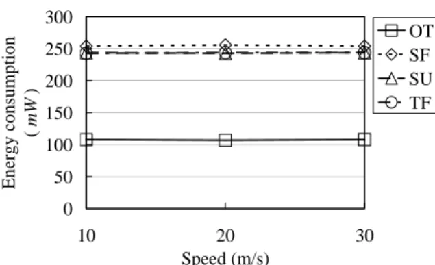
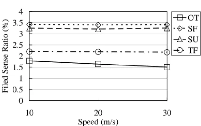
(7) first catching the target is shown in Fig. 10. When a source has caught the target, it must follow the mobile target closely. Therefore, a source must know the position of mobile target at any time and the query process is needed frequently. After the source has caught the target, it using TF protocol will need to issue the query packets frequently. This is because that the source is near the target and it must issue a flooding after it has reached the position of target. OT SF SU TF. 250 200 150 100 50 0 20 Speed (m/s). 30. 300. 1900 1800 1700 1600 1500 1400 1300 1200. OT SF SU TF. 200 150 100 50 10. 20 Speed (m/s). 30. Fig. 13: Average energy consumption before the source first catching the target at 1500 nodes. 10. 20 Speed (m/s). 30. 300. Fig. 11: The time of the first sensor energy exhausted at 1000 nodes. 3.5 Filed Sense Ratio (%). OT SF SU TF. 250. 0. OT SF SU TF. 3 2.5 2. OT SF SU TF. 250 200 150 100 50 0 10. 1.5 1. 20 Speed (m/s). 30. Fig. 14: Average energy consumption after the source first catching the target at 1500 nodes.. 0.5 0 10. 20 Speed (m/s). 30. Fig. 12: Failed sensor ratio at 1000 nodes. Next, we compare the time of first sensor energy exhausted in Fig. 11. The flooding query is used at a predefined period SU and SF protocols, so the speed of target can not influence the time of first sensor energy exhausted. OT protocol has better effect than the others while the velocity of source is higher than 20 m/s. This is because that the source will chase the target faster in 30 m/s and it does not need to issue the. Live Time ( Sec ). Live Time ( Sec ). Fig. 10: Average energy consumption after the source first catching the target at 1000 nodes.. Energy Consumption ( mW ). 10. Energy consumption ( mW ). Energy consumption ( mW ). 300. flooding query after it has caught the target. TF protocol in 30 m/s still needs to issue the flooding query persistently though the source is near the target. Finally, we compare failed sensor ratio in simulation time as shown in Fig. 12. The failed sensor ratio represents the ratio of sensor consumed. OT has better performance than the others. This is because that OT does not need track the target using the broadcast strategy. Therefore, it can reduce the power consumption than the others. The failed ratio decreases while the velocity of source increases. The results of 1500 sensors are similar to that of 1000 sensor. The average energy consumption before the source first catching the target is shown in Fig. 13.The average energy consumption after the source first catching the target is shown in Fig. 14.The time of first sensor energy exhausted is shown in Fig. 15. The failed sensor ratio in simulation time is shown Fig. 16.. 1900 1800 1700 1600 1500 1400 1300 1200. OT SF SU TF. 10. 20 Speed (m/s). 30.

(8) Filed Sense Ratio (%). Fig. 15: The time of the first sensor energy exhausted at 1500 nodes. 4 3.5 3 2.5 2 1.5 1 0.5 0. OT SF SU TF. [6]. [7]. [8]. [9]. 10. 20 Speed (m/s). 30. Fig. 16: Failed sensor ratio at 1500 nodes. From the experimental results, our proposed OT protocol has better performance than the other protocols based on flooding. Our proposed protocol can reduce the power consumption while it wants to query the location of target. When the source has caught the target and it wants to follow the target, our proposed protocol can save the power efficiently. Moreover, an adjusting face tracks process is proposed in our protocol. The source will follow the shorter path to chase the target. The adjusting face tracks process not only can shorten the length of tracks but also can avoid the track loop problem.. V. CONCLUSIONS In this paper, we proposed a dynamically tracking object protocol for sensor networks. Our proposed protocol can reduce the power consumption while it wants to query the location of target. And it also can avoid the track loop problem. The source will follow the shorter path to chase the target. From the experimental results, our proposed OT protocol has better performance than the other protocols based on flooding.. [10]. [11]. [12]. [13]. [14]. [15]. [16]. [17] [18]. REFERENCES [1]. [2]. [3]. [4]. [5]. R. R. Brooks and A. M. Sayeed, “Distributed Target Classification and Tracking in Sensor Networks,” in Proceedings of the IEEE, Volume 91, Number 8, pp. 1163-1171, August 2003. K. Bhaskar, B. W. Stephen, and B. Ramon, “Phase Transition Phenomena in Wireless Ad-Hoc Networks,” in Proceedings of IEEE GLOBECOM, Volume 5, pp.2921-2925, San Antonio, Texas, November 2001. Y.-S. Chen and S.-Y. Ann, “VE-Mobicast: A Variant-Egg-Based Mobicast Routing Protocol in Wireless Sensor Networks,” in Proceedings of the 40th IEEE International Conference on Communications (IEEE ICC 2005), Seoul, Korea, May 2005. W.-P. Chen, J. C. Hou, and L. Sha, “Dynamic Clustering for Acoustic Target Tracking in Wireless Sensor Networks,” in Proceeding of 11th IEEE International Conference on Network Protocols (ICNP'03), pp. 284-294, Atlanta, Georgia, USA, November 2003. C.-Y. Chong, F. Zhao, S. Mori, and S. Kumar, “Distributed Tracking in Wireless Ad Hoc Sensor Networks,” in Proceedings of the Sixth International Conference on. [19]. [20]. Information Fusion (FUSION 2003), pp. 431-438, Cairns, Australia, July 2003. L. J. Guibas, “Sensing, Tracking, and Reasoning with Relations,” IEEE Signal Processing Magazine, Volume 19, Number 2, pp.73-85, March 2002. S. Goel and T. Imielinski, “Prediction-based Monitoring in Sensor Networks: Taking Lessons from MPEG,” in ACM Computer Communication, Volume 31, Number 5, pp. 82-98, October 2001. Q. Huang, C. Lu, and G.-C. Roman, “Mobicast: Just-in-time multicast for sensor networks under spatiotemporal constraints,” in Proceeding of the 2nd International Workshop on Information Processing in Sensor Networks, pp. 442-457, Palo Alto, CA, USA, April 2003. Q. Huang, C. Lu, and G.-C. Roman, “Reliable Mobicast via Face-Aware Routing,” in Proceedings of the IEEE Conference on Computer Communications (INFOCOM'04), Hong Kong, China, March 2004. E. Kranakis, H. Singh, and J. Urrutia, “Compass Routing on Geometric Networks,” in Proceedings of 11th Canadian Conference on Computational Geometry, pp. 51-54, Vancouver, CANADA, August 1999. H. T. Kung and D. Vlah, “Efficient Location Tracking Using Sensor Networks,” in Proceedings of the IEEE Wireless Communications and Networking Conference (WCNC 2003), New Orleans, Louisiana, USA , March 2003. F. Kuhn, R. Wattenhofer, Y. Zhang, and A. Zollinger, “Geometric Ad-Hoc Routing: Of Theory and Practice,” in Proceedings 22nd ACM Symposium on the Principles of Distributed Computing (PODC 2003), pp. 63-72, Boston, Massachusetts, July 2003. C.-Y. Lin and Y.-C. Tseng, “Structures for In-Network Moving Object Tracking in Wireless Sensor Networks,” in Proceedings of the First International Conference on Broadband Networks (BROADNETS'04), pp. 718-727, San Jose, California, USA, October 2004. D. Li, K. D. Wong, Y. H. Hu, and A. M. Sayeed, “Detection, Classification, and Tracking of Targets,” IEEE Signal Processing Magazine, Volume19, Number 2, pp.17-30, March 2002. F. Mondinelli and Z. M. Kovacs-Vajna, “Self-Localizing Sensor Network Architectures,” IEEE Transactions on Instrumentation and Measurement, Volume 53, Number 2, pp. 277-283, April 2004. Y.-C. Tseng, S.-P. Kuo, H.-W. Lee, and C.-F. Huang, “Location Tracking in a Wireless Sensor Network by Mobile Agents and Its Data Fusion Strategies,” Computer Journal, Volume 47, Number 4, pp. 448-460, 2004. VINT Project, “Network Simulator version 2 (NS-2),” Technical report, http://www.isi.edu/nsnam/ns, June, 2001. Y. Xu, J. Winter, and W.-C. Lee, “Prediction-based Strategies for Energy Saving in Object Tracking Sensor Networks,” in Proceedings of the 2004 IEEE International Conference on Mobile Data Management (MDM’04), pp.346-357, Berkeley, California, January 2004. H. Yang and B. Sikdor, “A Protocol for Tracking Mobile Targets Using Sensor Network, Sensor Network Protocols and Applications,” in Proceedings of the 1st IEEE International Workshop on Sensor Network Protocols and Applications, pp.71-81, Anchorage, Alaska, May 2003. Y. Zou and K. Chakrabarty, “Target Localization Based on Energy Considerations in Distributed Sensor Networks,” in Proceedings of the 5st IEEE International Workshop on Sensor Network Protocols and Applications, pp.51-58, Anchorage, Alaska, May 2003..

(9)