On-Line Learning Delivery Decision Support System
for Highly Product Mixed Semiconductor Foundry
Chih-Yuan Yu and Han-Pang Huang, Member, IEEE
Abstract—A production learning system (PLS) based on the tool model was constructed as a decision support and real-time infor-mation update system to forecast the cycle time. A tool model in-cludes a waiting model and a processing model. Each of the waiting and processing models uses a backpropagation neural network to establish the relationship between the input and output (time) of the model. Hence, cycle time estimation, tool group move and con-firm line item performance (CLIP) value can be obtained based on the memory stored in the neural network. The result shows that the forecasting ability of the PLS has an error rate below 8% on average.
Index Terms—Backpropagation neural network (BPNN), cycle time estimation, decision support system, tool group move, tool model.
I. INTRODUCTION
T
HE FLOW of lots in an IC fab is like a job shop and very complex. To model an entire fab as a unit is a tremendous task. Connors [1] modeled different tool groups found in semi-conductor wafer fabrication using a queueing network. Kim [3], Juang [4], Lu [5] and Wein [8] also used queueing theory to an-alyze IC fabs. Vepsalainen and Morton [7] used an iterative pro-cedure to generate the average estimated remaining delay. Eht-eshami [2] used historical average cycle time and added safety margin to commit a product delivery date.All methods described above used an “average” feature. However, this feature cannot be used to characterize the attributes of each operation and waiting effects in detail. Thus, a tool model [9], which characterizes the dynamics of a single tool and considers the operation time as the prime unit, is proposed. Backpropagation neural networks (BPNN) have been widely used in several areas and proved to have the ability to model the nonlinear relationship of a dynamic system. As a result, BPNN was used in this paper to learn the relationship in each model [9].
Since the time of each step can be obtained, the estimated cycle time of a product is the summation of the time estimated by all tool models related to the operation flow of the product. The user can predict the cycle time of a product before it is released. The estimated remaining cycle time of a lot can help to see whether the lot is late for time delivery or not. The tool move
Manuscript received February 29, 2000; revised August 29, 2001. This work supported in part by the National Science Council, Taiwan, R.O.C., under Grant NSC 90-2212-E-002-222. This paper was presented in part at the National Con-ference on Automation Technology, ChiaYi, Taiwan, R.O.C., July 1999.
The authors are with the Robotics Laboratory, Department of Mechanical En-gineering, National Taiwan University, Taipei 10660, Taiwan, R.O.C. (e-mail: [email protected]).
Publisher Item Identifier S 0894-6507(02)04465-2.
suggestion can be a reference to re-configure the tool allocation within a day, while the confirm line item performance (CLIP) value represents the percentage of lots scheduled for output in a week.
II. TOOLMODEL ANDPRODUCTIONLEARNINGSYSTEM
Tools are the actual machines, while tool groups are virtual units used to define the flow of a product. Usually, one or more tools that perform the same operation belong to a tool group. The flow of a lot or a product is the sequence of the tool groups that define the operations (or tool groups) it takes but not the speci-fied tools. The lot flow is related to its product type or typically its route type. Hence, a lot after processing in the previous step only knows the next tool group that it should go. Any available tools belonging to the tool group can serve this lot. If no tool is available, this lot waits in some place we call a virtual tool group. Lots waiting in the same tool group will compete for the same resources, i.e., the tools.
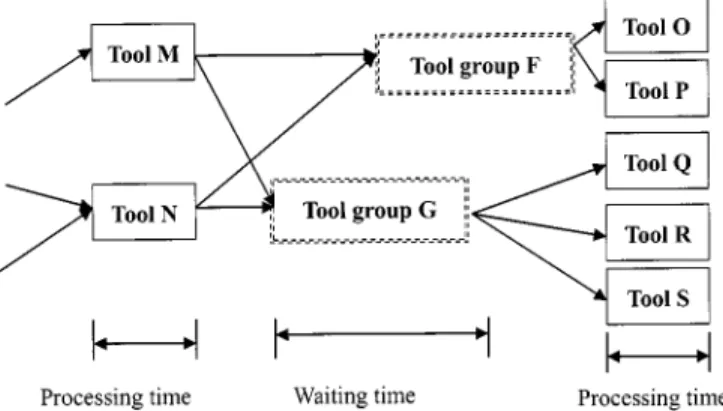
From the viewpoint of a lot, it takes about 200 to 300 steps to complete the process. The tool model attempts to divide the flow into the basic elements, or steps, rather than stages. The tool model concept involves building a model to determine the time required for a step for a lot. In detail, the tool model can be divided into two parts, the waiting part (wait in the tool group) and the processing part (processed in the tool). Since the tool model is divided into two parts, the lot flow in the tool model is a stream of waiting, processing, waiting, processing and so on. The relationships among the tool, the tool group and the lot flow can be further elaborated. Fig. 1 is a part of the topology of the tools and virtual tool groups in the fab. The tool group frame is dotted to represent the virtual condition. For example, tools O and P are the members of tool group F while tools Q, R, and S belong to tool group G. A lot K just finishing processing in tool M is forwarded to the next step, the tool group G. If tools Q, R, and S are busy, then the lot K waits in the tool group G, where there may have some waiting lots already. A higher priority lot will be chosen when a tool is free. Hence, the priority is a critical attribute for deciding the waiting time in a tool group. The cycle time of a lot is the summation of the time at each step as
CT (1)
where is the total numbers of steps for the lot . and are the waiting time and processing time in step , respectively.
Based on the decomposed tool model architecture, the scale and complexity of modeling are reduced enormously. A neural
Fig. 1. The relationships among tool, tool group, and lot flow.
Fig. 2. The architecture of BPNN.
network will be used to forecast the waiting time and processing time of both models.
Since neural networks have the properties of massively par-allel processing, high memory and learning abilities, they are capable of modeling the nonlinearity of a complex dynamic system. Hence, a BPNN shown in Fig. 2 was applied to predict the times in waiting and processing models. Since each model contains a BPNN, the number of BPNN for tool groups is equal to the number of tool groups, and the number of BPNN for tools is equal to the number of tools. In this paper, the fab under in-vestigation has about 200 tool groups and 500 tools.
To construct the waiting/processing time model, the first step is to determine the inputs of the network. There are 12 fac-tors chosen as the inputs of BPNN for waiting time model and one output represents the waiting time. The inputs are waiting wafers, priority of the lot, push index, pull index, month index, day index, time index, and waiting pods of five priorities (SH, H, R, N, S). The output is the actual waiting time in minute. As to the processing model, the most important attribute of the processing time is the recipe. It is very difficult to acquire the de-tailed information for each recipe. In our simulation data, tech-nology can also identify the recipe, which is used for the lot. Therefore, number of wafers and technology are chosen to clas-sify the time for one lot processed in a tool. The detailed descrip-tion of the attributes used in the waiting and processing models are listed in Tables I and II, respectively.
The production learning system (PLS) is an on line learning system for a full-scale fab to implement the tool model by ap-plying a backpropagation neural network. The PLS re-trains each model periodically. As a result, the models will reflect the changes in the shop floor as time goes by. Hence, the PLS is a dynamic learning system that provides real time information for the fab. The PLS client/server architecture is shown in Fig. 3.
The client program provides several functions. Based on the estimated time of each step, we can easily get the useful infor-mation, such as cycle time, tool group move, CLIP and so on. The computation time for those information is below 10 min in average. In contrast, the traditional method takes a long time to resimulate. The server program keeps running, while the client runs when necessary. The client can run at any place where the ODBC is connected to the computer that stores the memory of the neural network.
III. SIMULATION ANDRESULTS
The data used in the PLS is collected from a real fab by the server program. It takes about 3 days and 50 000 data sets for warming up the system and training the networks. The client program of the PLS provides the following functions: cycle time estimation of a product, remaining cycle time estimation of a lot, tool group move estimation and CLIP. These functions are described below.
A. Function I: Cycle Time Estimation of a Product
This function is used by marketing sales to obtain product cycle time estimation before receiving a new order. The sales simply input the product type, number of wafers and priority for the lots. The waiting time in the tool group and the pro-cessing time in the tool of each operation are calculated and then the total cycle time of the lot is a summation of this se-quence of steps. Even the lots belonging to a new route can be predicted because the time a lot spent in the fab depends upon the attributes mentioned above rather than the route. As long as the operation in each step has been learned before, the time of each step is still calculable.
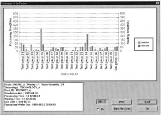
The estimated cycle time of a product A, which is a new order from a customer, is shown in Fig. 4. The waiting time and pro-cessing time of each operation are calculated and the forecasted wafer out information is also shown. Hence, if the product A is released at 1999-04-30 with priority “R” and with wafer quan-tity “24,” then the forecasted processing time is about 10.5 days while the lot takes 10.5 days to wait in the buffers. The fore-casted wafer out is earlier than the due date (1999-05-23). It means that this lot can be delivered on time. Based on this in-formation, the sales can guarantee the on-time delivery to the customer and accept this new order.
Furthermore, an unusual waiting time may indicate a bottle-neck. For example, the waiting time of the product in Fig. 4 in the tool group 85 is up to 360 minutes. It is strange that a lot with priority “R” will wait 6 hours in the tool group 85. The su-pervisor should check the capacity or the tool status in the tool group 85 in order to prevent the bottleneck occurrence.
The comparison of cycle time estimation is listed in Table III. For each product, the cycle time of 5 lots with priority “N” are averaged. There are different numbers of operation for each product. It is obvious that the error from the PLS can be below 8% in every product cycle time forecast.
B. Function II: Remaining Cycle Time Estimation of a Lot
Much previous research showed that the least slack (LS) policy and its variants could support better performance for
TABLE I
THEATTRIBUTESUSED IN THEWAITINGMODEL
TABLE II
THEATTRIBUTESUSED IN THEPROCESSINGMODEL
Fig. 3. The client/server architecture of the PLS.
reducing the cycle time mean and variance. In these least slack policies, the term “estimated remaining cycle time” is the key
component because of its indeterminacy. A good estimated remaining cycle time could support the accuracy of LS and
Fig. 4. Estimation of a product cycle time.
TABLE III
THEERRORS OFFORECASTEDPRODUCTCYCLETIMES
then enhance the on-time delivery. The manager can adjust the priorities of the lots that may be too late or too early to commit their due date based on the estimated remaining cycle time from the PLS. The formulation of calculating remaining cycle time of a lot is just modified from Eq. (1) as
(2)
where is the last finished step.
The remaining cycle time estimation can be used to support the decision system, as shown in Fig. 5. The supervisor can de-tect the lots that may be delayed, and then change the priorities of these lots for on-time delivery.
The comparison of the forecasted remaining cycle time (RCT) and the actual RCT is given in Table IV. The forecasts of LOT A, LOT D, and LOT F are almost perfect, while the others are larger. Nevertheless, the forecasts of product cycle time and the remaining cycle time are both close to the actual value. This can ensure the correctness of the forecast and then
Fig. 5. The architecture of the closed-loop cycle time forecasting system based on the tool model.
promise the reliability of the derived function (tool group move and CLIP).
C. Function III: Tool Group Move Estimation
If the tool group move of the tool group M is N, it means that there are N wafers processed through the tool group M. Tool group move is defined as the number of lots completing an op-eration. For example, if a lot with 24 wafers has been processed by the tool group M, then 24 tool group moves are added to the tool group M. Usually, the calculation interval of the tool group move of tool groups is 1 day. The supervisor watches the fore-casted tool group moves of all tool groups and may reconfigure the target throughput of each tool group.
D. Function IV: CLIP
CLIP is an important index to reflect on-time delivery. The general definition of CLIP is the number of products deliv-ered on schedule over the number of products that should be delivered on schedule within a specified interval, say, for ex-ample, seven days. According to the estimated remaining cycle time of lots, the forecasted CLIP, which only includes the lots
TABLE IV
FORECASTEDREMAININGCYCLETIME OFLOTS
whose due dates are less than seven days, can be obtained. This function can provide the status of urgent lots that are due to be shipped within seven days. A typical CLIP calculated on 1999-04-30 is about 0.86. It means that 86% product whose due date are within the next seven days can be delivered on time. If the forecasted CLIP is too low, the delayed lots should be ad-justed to higher priorities in order to commit due date.
IV. CONCLUSION
In order to model a fab in detail, a step instead of a stage was chosen as the fundamental unit of the fab model. The proposed tool model is used to forecast the time of each step. According to the different attributes of the waiting time and processing time, the tool model is divided into two parts, a waiting model and a processing model. A backpropagation neural network was ap-plied to learn the input-output relationship of both submodels.
Based on the tool model, the estimated cycle time of a product before releasing, estimated remaining cycle time for a lot, tool move and CLIP can be obtained. The results show that the on-line learning system, PLS, which on-line updates the new information of the fab, has a good forecasting ability with less error. In particular, each function of the PLS can provide useful information for the supervisor or manager to make better decisions. Less computation time is another feature of the PLS.
ACKNOWLEDGMENT
The assistance from the Taiwan Semiconductor Manufac-turing Company (TSMC) is greatly appreciated.
REFERENCES
[1] D. P. Connors, G. E. Feigin, and D. D. Yao, “A queueing network model for semiconductor manufacturing,” IEEE Trans. Semiconduct.
Manu-fact., vol. 9, pp. 412–426, Aug. 1996.
[2] B. Ehteshami, R. G. Petrakian, and P. M. Shabe, “Trade-off in cycle time management: Hot lots,” IEEE Trans. Semiconduct. Manufact., vol. 5, pp. 101–106, May 1992.
[3] Y. D. Kim, J. U. Kim, S. K. Lim, and H. B. Jun, “Due-date based scheduling and control policies in a multiproduct semiconductor wafer fabrication facility,” IEEE Trans. Semiconduct. Manufact., vol. 11, pp. 155–164, Feb. 1998.
[4] J. Y. Juang and H. P. Huang, “Queueing network analysis for an IC foundry,” in Proc. 2000 IEEE Int. Conf. Robotics and Automation, San Francisco, CA, Apr. 2000, pp. 3389–3394.
[5] C. H. Lu, D. Ramaswamy, and P. R. Kumar, “Efficient scheduling policies to reduce mean and variance of cycle-time in semiconductor manufacturing plants,” IEEE Trans. Semiconduct. Manufact., vol. 7, pp. 374–388, Aug. 1994.
[6] S. H. Lu and P. R. Kumar, “Distributed scheduling based on due dates and buffer priorities,” IEEE Trans. Automat. Contr., vol. 36, no. 12, pp. 1406–1416, 1991.
[7] A. P. J. Vepsalainen, “Improving local priority rules with global lead-time estimates: A simulation study,” J. Manufact. Oper. Mgmt., vol. 1, pp. 102–118, 1988.
[8] L. M. Wein, “Scheduling semiconductor wafer fabrication,” IEEE Trans.
Semiconduct. Manufact., vol. 1, pp. 115–130, Aug. 1988.
[9] C.Y. Yu and H. P. Huang, “Fab model based on distributed neural net-work,” in Proc. Nat. Conf. Automation Technology, ChiaYi, Taiwan, R.O.C., 1999, pp. 271–277.
Chih-Yuan Yu was born in Chang-Hua, Taiwan,
R.O.C., in 1975. He received the B.Eng. degree in 1997 from National Taiwan University and is currently working toward the Ph.D. degree in mechanical engineering at the National Taiwan University, Taiwan, R.O.C.
His research interests include factory automation, enterprise integration, scheduling and dispatching, supply chain management, intelligent control and distributed multi-agents.
Mr. Yu received the “Nomination for Kayamori Best Paper Award” in 2001 IEEE International Conference on Robotics and Automation.
Han-Pang Huang (S’83–M’86) graduated from
National Taipei Institute of Technology in 1977, and received the M.S. and Ph.D. degrees in electrical engineering from The University of Michigan, Ann Arbor, in 1982 and 1986, respectively.
Since 1986, he has been with the National Taiwan University, where he is currently a Professor in the Department of Mechanical Engineering and Graduate Institute of Industrial Engineering. He was the Vice Chairperson of the Mechanical Engineering Department from August 1992 to July 1993, the Director of Manufacturing Automation Research Technology Center from August 1996 to July 1999. Currently, he is the Associate Dean of College of Engineering, National Taiwan University. His research interests include machine intelligence, network-based manufacturing systems, intelligent robotic systems, prosthetic hands, nanomanipulation and nonlinear systems.
Dr. Huang is a member of Tau Beta Pi, SME, CFSA, CIAE. He was the Editor-in-Chief of the Journal of Chinese Fuzzy System Association, the Pro-gram Chair of the 1998 International Conference on Mechatronic Technology (ICMT’98), and the General Vice Chair of the Eighth International Fuzzy Sys-tems Association World Congress (IFSA’99), 1999. He is the Organizing Com-mittee Chair of the 2002 Asian Pacific Industrial Engineering Conference. He is the co-author of the book Fuzzy Neural Networks: Mathematical Foundation
and its Applications in Engineering (Boca Raton, FL: CRC) in January 2001.
He was the Guest Editor of IEEE/ASME TRANSACTIONS ONMECHATRONICSin 2001. Currently, he is the Editor-in-Chief of the International Journal of Fuzzy
Systems. He has received three-time Distinguished Research Awards from