量子與光學同調波之研究:利用微晶體雷射研究空間模態與極化奇異點特徵

國

立

交

通

大

學

電子物理系

博

士

論

文

量子與光學同調波之研究:

利用微晶體雷射研究空間模態與極化奇異點特徵

Study of Quantum and Optical Coherent Waves: Pattern Formation

and Polarization Singularities Generated from Microchip Laser Cavity

研 究 生：陸亭樺

指導教授：陳永富 教授

Study of Quantum and Optical Coherent Waves: Pattern Formation

and Polarization Singularities Generated from Microchip Laser Cavity

研 究 生：陸亭樺

Student：Ting-Hua Lu

指導教授：陳永富

Advisor：Yung-Fu Chen

國 立 交 通 大 學

電子物理研究所

博 士 論 文

A Thesis

Submitted to Institute of Electrophysics College of Science

National Chiao Tung University in partial Fulfillment of the Requirements

for the Degree of PhD

in

Electrophysics

May 2008

學生: 陸亭樺 指導老師: 陳永富教授

國立交通大學電子物理系博士班

摘要

本論文係用微晶體雷射的空間模態研究同調光波的量子與古典對應關係以及極化 向量場中奇異點的特徵。由於雷射共振腔在近軸近似下的波函數解與量子簡諧運動有異 曲同工的數學形式，因此深入研究量子簡諧運動為本論文中相當重要的基石。首先我們 以一維 Schrödinger 同調態出發並推廣至二維系統。經由縝密的分析與思考得到符合共 振腔條件的廣義同調態，藉此與實驗中所見之有趣的光學物理現象做一番連接。進一步 研究發現共振腔中縱向與橫向的頻率耦合與模態鎖定的結果所顯示的”魔梯”現象。這一 類的空間模態不僅帶領我們進入鮮少被探討的雷射領域更提供了介於微觀與宏觀之間 的綜觀領域一些相關研究方向。再者，針對實驗結果的理論分析更顯示了這些空間模態 擁有很大的角動量，這對於未來的雷射技術提供了一些前瞻性的想法。 本文另一個重點是探討極化向量場中奇異點的特徵。極化奇異點的形態與光場本身 的模態密不可分且相依相生。文中利用半球形共振腔產生光與增益介質之交互作用使得 空間模態衍生出極化糾纏的實驗結果。透過嚴謹的理論分析不僅完整地重建出光波之空 間模態，且各種極化奇異點特徵的有趣面貌亦被清楚地呈現。對於極化奇異點的深入研 究除了能夠更了解光波的特性也對光波的應用層面提供了值得思考的方向。

from Microchip Laser Cavity

Student: Ting-Hua Lu Advisor: Prof. Yung-Fu Chen

Institute and Department of Electrophysics National Chiao Tung University

ABSTRACT

This thesis presents several novel optical experiments which provide fresh insights for quantum-classical correspondence with pattern formation and polarization characteristics of light by use of microchip laser cavity. Quantum physics was developed substantially after Schrödinger proposed his important coherent states of quantum harmonic oscillator. Harmonic oscillator is the analogue of spherical laser cavity in our system. We start from one-dimensional Schrödinger coherent states and broaden the theory to two-dimensional problem to be related to our laser system under paraxial approximation.

We not only develop a general form to elucidate various kinds of states completely in the laser system which is slightly disturbed by coupling with environment but also extract the coherent states in the degenerate cavity of longitudinal-transverse coupling. In addition to the eigenstates in laser cavity, the three-dimensional coherent waves exhibit the classical-like feature on the transverse patterns in virtue of nonlinear optical effects. We verify that the specific phenomenon leads to “Devil’s staircase” which is demonstrated in other physical regime but firstly found in laser cavity. Furthermore, the analytic results have good agreement with experimental patterns and provide efficient approach to understand the nature of coherent waves in the cavity. With the theoretical results, the coherent waves are found to carry large angular momentum and may provide some applications in laser technique.

Another topic in this thesis is polarization singularity in laser cavity. Besides phase singularity in complex scalar waves which provide some unique applications, polarization singularities also play a vital role such as the skeleton in vector waves for the study of optical fields. We employ the hemispherical cavity to generate vector fields. After precise measurement and deliberate analysis, the variation of polarization singularities embedded in high-order vector laser waves can be realized. Interestingly, the polarization singularities are discovered as fascinating patterns accompany with vector fields. Studying the structures of the polarization singularities in coherent vector fields may help us to understand the nature of the waves and provide insights in application.

是我們選擇了生活，還是生活選擇了我? 離開家鄉北上求學的我總不時地想到小時 候頂著大熱天在市場幫忙工作的情境，當時只覺得媽媽工作很辛苦，生活卻過得不算輕 鬆。小小年紀就想著在未來的日子我一定要有機會選擇讓自己快樂的生活方式。然而父 母親告訴我，對於處在貧窮中的小孩，只有讀書才有機會讓自己的生活改變。在那些為 聯考奮戰的日子裡，這句話始終在我心頭迴盪。如願考上交大也順利畢業，畢業後跟著 大多數人的腳步踏入研究所，心想再充實兩年就可以去園區工作，完成小時候的夢想。 天知道命運的安排卻是如此微妙，就差那麼一點，我就與美麗的物理世界擦身而過。 從四年多前陳永富教授答應收我為碩士生的那天開始，原來我的人生已經開始了另 一段自己從未預期的旅程。大四的下學期是我大學生活中最充實的一段時光，因為每個 禮拜陳教授都願意教導我做研究的方法與知識。我在陳教授身上看到了教學的熱誠與研 究的態度，這的確深深地感動了我，同時也潛移默化著我的想法。真正進入研究所後， 除了陳教授以外還有與陳教授合作的黃凱風教授一起參與。黃教授是個很有風範的學 者，對學術認真地投入，經常與我討論實驗的結果幫助我釐清許多研究上的困惑。在兩 位教授的帶領之下，漸漸地我也能感受到物理的魅力與它帶給我的感動。我終於明白為 什麼他們會不停地討論所看到的實驗現象、不斷地指導我讓我了解事物的真理，這是沒 有用心投入過的人所不會了解的。從一個陌生的實驗結果要走到完全了解它背後所隱藏 的意義是一條很漫長的路，路上總有些崎嶇與阻礙，我很幸運地有兩位良師的指導讓我 能克服種種困難。不管是面臨研究上或是生活上的挫折，我都很感謝他們一再地鼓勵 我、一再地給我機會，扮演我生命中的貴人。畢業只是一個轉折點，我會帶著在兩位老 師身上所學到的精神與態度繼續探索這美麗的世界，期盼未來能不負他們的期望。 這四年來我得到許多人的幫助:從剛進入實驗室建勳學長、意鑫學長和怡君學姊的 指導，到真正動手做實驗時蘇老大和 01 學姊的協助讓我學到許多寶貴知識。有寶妹、 歐大戶、廖ㄟ、王胖、哲彥、小黃、國欽學長、思武學長和春蘜學姊的陪伴更充實了研 究生活。還有實驗室裡的依萍、雅婷、恩毓、建誠、興弛、紀暐、彥廷、漢龍學長、柏 祥學長、毓捷、建至、郁仁，能與他們共度實驗室的珍貴時光令我感到非常開心。更要 感謝口試委員給我的指導讓我獲益良多。 在即將結束學生生涯之際，我特別要感謝我的家人無怨無悔地支持我。外公外婆和 奶奶的疼愛、父親的鼓勵、妹妹的幫忙、尤其是母親從小到大給我的身教讓我學會感恩 和惜福，母親一直是我努力向前的動力與典範。更要感謝七年來一直在我身邊給我無限 包容和體貼的東賢，能一起分享生活中的點滴是我最大的幸福。最後，感謝上天讓我有 機會選擇最適合自己的方式來成就我年輕歲月中最美好的時光。

摘要 ．．．．．．．．．．．．．．．．．．．．．．．．．．．．．．．．．．．．．． i

Abstract ．．．．．．．．．．．．．．．．．．．．．．．．．．．．．．．．．．．．．． ii

誌謝 ．．．．．．．．．．．．．．．．．．．．．．．．．．．．．．．．．．．．．． iii

Contents ．．．．．．．．．．．．．．．．．．．．．．．．．．．．．．．．．．．．．． iv

List of Figures ．．．．．．．．．．．．．．．．．．．．．．．．．．．．．．．．．．． vii

Chapter 0

．．．．．．．．．．．．．．．．．．．．．．．．．．．．．．．．． 1

Introduction:

Guide to the Main Text

Chapter 1

．．．．．．．．．．．．．．．．．．．．．．．．．．．．．．．．． 3

Classical and Quantum Harmonic Oscillators

1.1 One-dimensional Harmonic Oscillator ．．．．．．．．．．．．．．．．．．．．． 3 1.2 Two-dimensional Harmonic Oscillator ．．．．．．．．．．．．．．．．．．．．． 7 1.3 Schrödinger Coherent States of the 1D Harmonic Oscillator ．．．．．．．．．．． 10 1.4 Stationary Coherent States of 2D Harmonic Oscillator ．．．．．．．．．．．．．． 14 1.5 Unitary Transformation between Stationary States and wave packet states．．．．． 23

REFERENCES．．．．．．．．．．．．．．．．．．．．．．．．．．．．．．．．．．． 28

Chapter 2

．．．．．．．．．．．．．．．．．．．．．．．．．．．．．．．．． 29

Eigenstates of Harmonic Oscillator and Spherical Laser Cavity

:

Generalized Coherent States and Polarization-entangled Patterns

2.1 Paraxial Approximation of Maxwell’s Equations．．．．．．．．．．．．．．．．． 29 2.2 The Generalized Coherent States:

Between Hermite-Gaussian and Laguerre-Gaussian modes．．．．．．．．．．．． 38 2.3 Generation of Polarization-entangled Optical Coherent Waves．．．．．．．．．． 48 2.3.1 Experimental Setup and Results．．．．．．．．．．．．．．．．．．．．．． 50 2.3.2 Analytical Wave Functions for Experimental Polarization-entangled

Patterns．．．．．．．．．．．．．．．．．．．．．．．．．．．．．．．．．．59

2.3.3 Summary．．．．．．．．．．．．．．．．．．．．．．．．．．．．．．．．． 73

Three-dimensional Optical Coherent Waves with

Longitudinal-transverse Coupling

3.1 Frequency Locking, Mode Locking, and Resonance ．．．．．．．．．．．．．．． 77 3.2 Devil’s Staircase with Two Competing Frequencies ．．．．．．．．．．．．．．． 77 3.3 Three-dimensional Coherent Waves Demonstrated from Laser Cavity ．．．．．．． 80

3.3.1 Theoretical Analysis for the Resonator ．．．．．．．．．．．．．．．．．． 80 3.3.2 Experimental Setup and Results ．．．．．．．．．．．．．．．．．．．．．． 86

3.3.3 Summary ．．．．．．．．．．．．．．．．．．．．．．．．．．．．．．．． 91

3.4 Spatially Localized Patterns Generated from Macroscopic Superposition of 3D

Coherent Laser Waves．．．．．．．．．．．．．．．．．．．．．．．．．．．．．． 97 3.4.1 Experimental Setup and Results ．．．．．．．．．．．．．．．．．．．．．． 98 3.4.2 Analysis and Theoretical Results．．．．．．．．．．．．．．．．．．．．．． 102 3.4.3 Summary ．．．．．．．．．．．．．．．．．．．．．．．．．．．．．．．．． 107

REFERENCES ．．．．．．．．．．．．．．．．．．．．．．．．．．．．．．．．．． 108

Chapter 4

．．．．．．．．．．．．．．．．．．．．．．．．．．．．．．．．． 111

Polarization Singularities in Hemispherical Cavity

4.1 Polarization and Stokes Parameter ．．．．．．．．．．．．．．．．．．．．．．． 111 4.2 Polarization Singularities．．．．．．．．．．．．．．．．．．．．．．．．．．．． 121 4.3 Generalized Structures of Polarization Singularities in Laguerre- Gaussian

Vector fields．．．．．．．．．．．．．．．．．．．．．．．．．．．．．．．．．． 122 4.3.1 Experimental setup and results ．．．．．．．．．．．．．．．．．．．．．． 122 4.3.2 Analytical Wave Functions for Experimental Patterns and Polarization

Singularities ．．．．．．．．．．．．．．．．．．．．．．．．．．．．．．． 128 4.3.3 Summary．．．．．．．．．．．．．．．．．．．．．．．．．．．．．．．．． 144 REFERENCES ．．．．．．．．．．．．．．．．．．．．．．．．．．．．．．．．．． 145

Chapter 5

．．．．．．．．．．．．．．．．．．．．．．．．．．．．．．．．． 148

Optical Waves Carrying Large Angular Momentum in Degenerate

Cavity

5.1 Angular Momentum of Electromagnetic Fields．．．．．．．．．．．．．．．．．．148 5.2 Linked and Knotted Coherent Laser Waves with Large Angular Momentum．．．． 151 5.2.1 Experimental Setup and Results ．．．．．．．．．．．．．．．．．．．．． 151 5.2.2 Analyses of Angular Momentum for Two Degenerate Coherent States．．．． 163

Chapter 6

．．．．．．．．．．．．．．．．．．．．．．．．．．．．．．．．． 170

Summary

and

Future

Work

Curriculum Vitae

．．．．．．．．．．．．．．．．．．．．．．．．．．．．．．．． 172

probability density of several states) Fig. 1.2.1 (a) The description of the potential of 2D harmonic oscillator. (b) Lissajous

figures with different frequency ratio and phase. (c) The eigenstates of 2D quantum harmonic oscillator with different orders.

Fig. 1.3.1 (a) Sixtieth excited state of 1D harmonic oscillator (b) 1D coherent state moving with time

Fig. 1.4.1 Comparison between the quantum stationary state , 2 , , (ξx,ξy;A,φ) q p u u N x y Φ [(a)-(c)]

and the classical Lissajous orbits [(a’)-(c’)] for the system of p:q=2:1 with 40

=

N , A=5.2 and (a) φ=0, (b) φ =0.3π, and (c) φ=0.6π.

Fig. 1.4.2 The same as Fig. 1.4.1 for the system of p:q=3:2 with N =22, A=5.2 and (a) 0

=

φ , (b) φ =0.3π, and (c) φ=0.6π.

Fig. 1.4.3 The same as Fig. 1.4.1 for the system of p:q=4:3 with N =15, A=5.2 and (a) 0

=

φ , (b) φ =0.3π, and (c) φ=0.6π.

Fig. 1.4.4 (a) Upper: wave patterns of stationary coherent states for N=20 with different values of the parameters φ. Lower: standing wave patterns corresponding to upper figures. (b) Upper: wave patterns of stationary coherent states for N=20 with different values of the parameters A . Lower: standing wave patterns

corresponding to upper figures.

Fig. 1.5.1 (a) The 1D wave packet states with M =5 and n=0~4 respectively. (b) The 1D stationary states with M =5 and m=0~4 respectively.

Fig. 1.5.2 The 2D time-independent stationary states with M =7 and n=0~6 respectively.

Fig. 1.5.3 The 2D eigenstates with M =7 and m=0~6 respectively.

Fig. 2.1.1 (a) Hermite-Gaussian modes with different index (m , n). (b) Standing waves of Laguerre-Gaussian modes with different index (l , p)

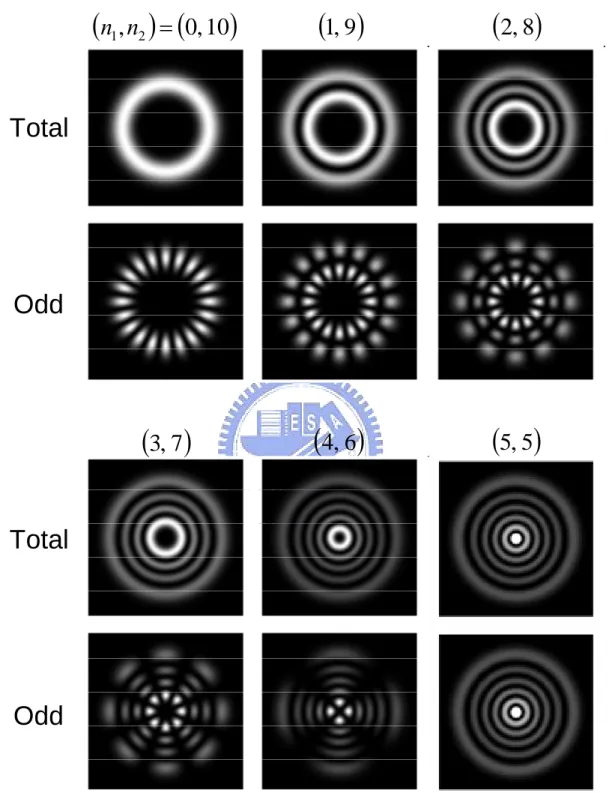
Fig. 2.2.1 The wave functions with different

(

n₁, n₂

)

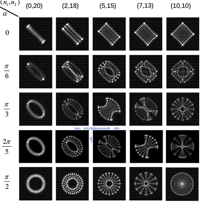
of a charged particle in a harmonic oscillator with uniform magnetic field.

Fig. 2.2.2 Numerical patterns of the GCSs with different phase factor and different order. Fig. 2.3.1 Experimental setup for the generation of polarization-entangled transverse modes

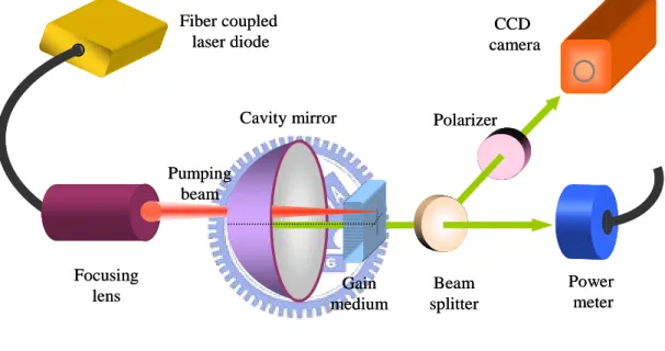
with off-axis pumping scheme in a highly isotropic diode-pumped microchip laser. 9 13 19 20 21 22 25 26 27 37 46 47 51

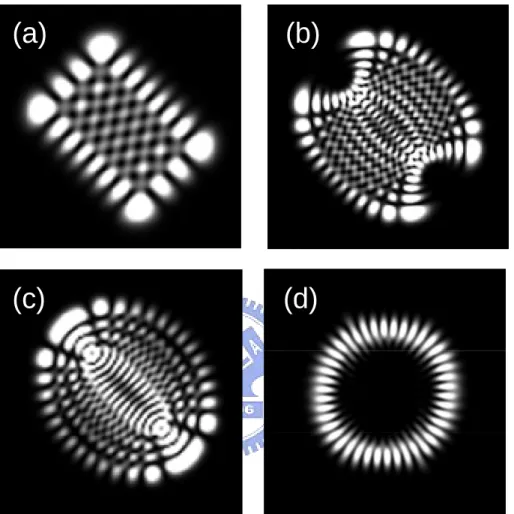
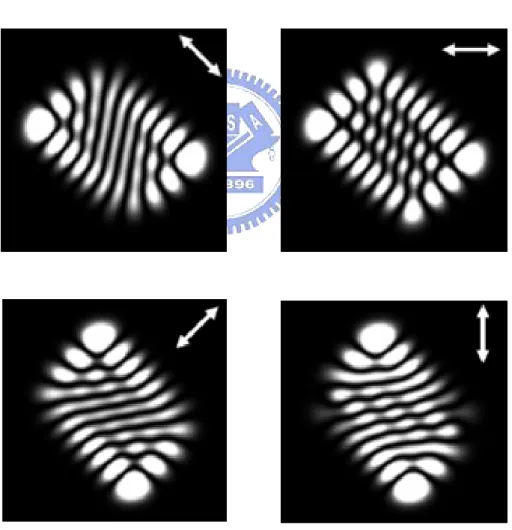
Fig. 2.3.3 Upper: Square experimental polarization-resolved patterns (a) 45 polarization(b) 900 polarization (c) 1350 polarization, (d) 1800polarization

Fig. 2.3.4 Upper: Hyperbolic experimental polarization-resolved patterns (a) 450 polarization (b) 900 polarization (c) 1350 polarization, (d) 1800polarization

Fig. 2.3.5 Upper: Elliptical experimental polarization-resolved patterns (a) 450 polarization (b) 900 polarization (c) 1350 polarization, (d) 1800polarization

Fig. 2.3.6 Upper: Circular experimental polarization-resolved patterns (a) 450 polarization (b) 900 polarization (c) 1350 polarization, (d) 1800polarization

Fig. 2.3.7 Numerically reconstructed patterns for the experimental results shown in Fig. 2.3.2.

Fig. 2.3.8 (a) The overlap functional I( )ϕ as a function of ϕ for the state E x y zv_x( , , ) in Eq. (2.3.6). (b) The overlap functional I( )ϕ as a function of ϕ for the state

( , , )

x

E x y zv in Eq. (2.3.8).

Fig. 2.3.9 Numerically reconstructed patterns for the experimental results shown in Fig. 2.3.3.

Fig. 2.3.10 Numerically reconstructed patterns for the experimental results shown in Fig. 2.3.4.

Fig. 2.3.11 Numerically reconstructed patterns for the experimental results shown in Fig. 2.3.5.

Fig. 2.3.12 Numerically reconstructed patterns for the experimental results shown in Fig. 2.3.6.

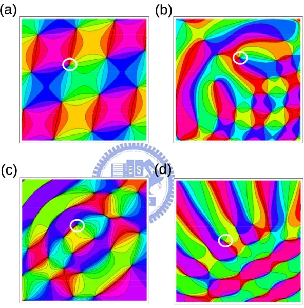
Fig. 2.3.13 Contour plot of angle field Θ( , )x y according to the reconstructed patterns in Fig. 2.3.7.

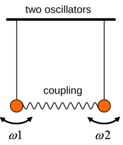
Fig. 2.3.14 Contour plot of angle field Θ( , )x y for the boxed regions shown in Fig. 2.4.13. Fig. 3.2.1 Two oscillators of different frequencies with some coupling strength

Fig. 3.2.2 Results of circle map with different coupling strength.

Fig. 3.3.1 A portion of the spectrum f(l,n,m) as a function of the bare mode-spacing ratio Ω for the range of 10≤ l ≤30and 200≤(m+n)≤ .

Fig. 3.3.2 Upper: an example for the Lissajous parametric surface described in equation (3.3.6) for the range fromz=−L 2 to z=L 2 with (p,q)=(3,2), P=2 and

0 0 =

φ . Bottom: the tomographic transverse patterns along the longitudinal axis. 55 56 57 58 62 65 66 67 68 69 71 72 79 79 82 85

Fig. 3.3.4 Experimental tomographic transverse patterns inside the cavity observed at 422 . 0 ≈ Ω .

Fig. 3.3.5 Bottom: Experimental mode-locked ratio P Q as a function of the bare 5ode-spacing ratio Ω. Upper: experimental far-field patterns observed in the mode-locked plateau with P Q=2/5.

Fig. 3.3.6 Experimental tomographic transverse patterns inside the cavity observed at 573

. 0 ≈

Ω .

Fig. 3.3.7 Bottom: Experimental mode-locked ratio P Q as a function of the bare 5ode-spacing ratio Ω. Upper: experimental far-field patterns observed in the mode-locked plateau with P Q=1/3.

Fig. 3.3.8 Bottom: Experimental mode-locked ratio P Q as a function of the bare 5ode-spacing ratio Ω. Upper: experimental far-field patterns observed in the mode-locked plateau with P Q=1/4.

Fig. 3.3.9 Bottom: Experimental mode-locked ratio P Q as a function of the bare 5ode-spacing ratio Ω. Upper: experimental far-field patterns observed in the mode-locked plateau with P Q=2/7.

Fig. 3.4.1 Photograph of the experimental laser cavity.

Fig. 3.4.2 Typical experimental far-field patterns observed in different cavity lengths for different indices ( , ;p q P Q . / )

Fig. 3.4.3 Upper: Numerical results of 3D coherent modes according to different transverse orders. Bottom: Numerical results of the superposition from the coherent modes with different orders.

Fig. 3.4.4 (a) Experimental tomographic transverse patterns inside the cavity observed at 0.84

Ω ≈ . (b) Numerical results corresponding to (a).

Fig. 3.4.5 Experimental strong spatially localized patterns with different ( , ; / )p q P Q .

Fig. 4.1.1 The evolution of the electric field vector leads to different kinds of polarization states: (a) Linear, (b) Circular, (c) Elliptical.

Fig. 4.1.2 Three kinds of polarization states of high-order transverse modes: (a) Azimuthally polarized, (b) Circularly polarized, (c) Radially polarized.

Fig. 4.1.3 The Poincaré representation of polarized light on a sphere.

Fig. 4.3.1 Experimental setup for the generation of propagation-dependent polarization 90 92 93 94 95 96 99 101 103 105 106 114 115 120 124

azimuthal index l: (a) (0, 9), (b) (0, 23), (c) (1, 39), (d) (1, 66), (e) (2, 41), (f) (7, 100).

Fig. 4.3.3 Polarization-resolved transverse patterns for the experimental result at three different propagation positions: z =0, z= zR, and z>>zR: (a) corresponding

to Fig. 4.3.2 (b) where z_R =1.26mm. (b) corresponding to Fig. 4.3.2 (c) where 28

. 1 =

R

z mm. The arrows indicate the transmission axis of the polarizer. z=z_R, and z>> z_R, where z_R =1.28mm.

Fig. 4.3.4 (a) Numerically reconstructed patterns for the experimental results shown in Fig. 4.3.3 (a), (b) Numerically reconstructed patterns for the experimental results shown in Fig. 4.3.3 (b).

Fig. 4.3.5 Structure of the C line singularities of the theoretical vector field from the view of propagation direction to the beam waist with the same radial index p=0 and different azimuthal index l: (a) (p, l)=(0, 1); (b) (p, l)=(0, 2); (c) (p, l)=(0, 3); (d) (p, l)=(0, 4); (e) (p, l)=(0, 5); (e) (p, l)=(0, 6).

Fig. 4.3.6 Structure of the C line singularities of the theoretical vector field from the view of propagation direction to the beam waist with the same radial index p=0 and different azimuthal index l: (a) (p, l)=(1, 1); (b) (p, l)=(1, 2); (c) (p, l)=(1, 3); (d) (p, l)=(1, 4); (e) (p, l)=(1, 5); (e) (p, l)=(1, 6).

Fig. 4.3.7 Structure of the C line singularities of the theoretical vector field from the view of propagation direction to the beam waist with the same radial index p=0 and different azimuthal index l: (a) (p, l)=(2, 1); (b) (p, l)=(2, 2); (c) (p, l)=(2, 3); (d) (p, l)=(2, 4); (e) (p, l)=(2, 5); (e) (p, l)=(2, 6).

Fig. 4.3.8 Numerical patterns of the angle function at the far field of the same radial index

p=0 and different azimuthal index l: (a) (p, l)=(0, 1); (b) (p, l)=(0, 2); (c) (p, l)=(0,

3); (d) (p, l)=(0, 4); (e) (p, l)=(0, 5); (e) (p, l)=(0, 6).

Fig. 4.3.9 Numerical patterns of the angle function at the far field of the same radial index

p=0 and different azimuthal index l: (a) (p, l)=(1, 1); (b) (p, l)=(1, 2); (c) (p, l)=(1,

3); (d) (p, l)=(1, 4); (e) (p, l)=(1, 5); (e) (p, l)=(1, 6).

Fig. 4.3.10 Numerical patterns of the angle function at the far field of the same radial index

p=0 and different azimuthal index l: (a) (p, l)=(2, 1); (b) (p, l)=(2, 2); (c) (p, l)=(2,

3); (d) (p, l)=(2, 4); (e) (p, l)=(2, 5); (e) (p, l)=(2, 6).

Fig. 4.3.11 (a) Experimental far-field pattern with radial and azimuthal index (p, l)=(1, 12). (b) Structure of C line singularities of the correspondent 3D vector field. (c) Structure of the C line singularities from the view of propagation direction to the beam waist. (d) Numerical pattern of the angle function at the far field.

Fig. 4.3.12 Diagram of the representation of the polarization state under propagation corresponding to the singularities of C lines (blue line), V points (white points at

127 130 133 134 135 137 138 139 141 143

to far field with Ω

=

1 4, ( , )p q

=

(2, 2). The pump position is at (0.29 mm, 0.30 mm); (b) Experimental tomographic transverse patterns for the range from beam waist to z=2.75L with Ω

=

1 3, ( , )p q

=

(3, 3). The pump position is at (0.23 mm, 0.30 mm).

Fig. 5.2.3 Experimental tomographic transverse patterns for the range from beam waist to far field with Ω

=

2 7, ( , )p q

=

(2, 5). The pump position is at (0.22 mm, 0.32 mm).

Fig. 5.2.4 (a) Numerical tomographic transverse patterns corresponding to Fig. 5.2.2 (a) with Eq. (5.2.1) and the parameters of (mo,no)=(110,110), ( , )p q =(2, 2),

1 4

P Q= , 0φo = and M =13. (b) (a) Numerical tomographic transverse

patterns corresponding to Fig. 5.2.2 (b) with Eq. (5.2.1) and the parameters of ) 140 , 60 ( ) , (mo no = , ( , )p q =(3,3), P Q=1 3, 0φo = and M =8.

Fig. 5.2.5 Numerical tomographic transverse patterns corresponding to Fig. 5.2.3 with Eq. (5.2.1) and the parameters of (m_o,n_o)=(60,130), ( , )p q =(2, 5), P Q=2 7,

0 =

o

φ and M =5.

Fig. 5.2.6 (a) Numerical tomographic transverse patterns corresponding to Fig. 5.2.2 (a) with Eq. (5.2.3) and the parameters of (m_o,n_o)=(110,110), ( , )p q =(2, 2),

1 4

P Q= , ϕ π= 2 and M =13. (b) (a) Numerical tomographic transverse patterns corresponding to Fig. 5.2.2 (b) with Eq. (5.2.3) and the parameters of

) 140 , 60 ( ) , (m_o n_o = , ( , )p q =(3,3), P Q=1 3, ϕ π= 2 and M =8.

Fig. 5.2.7 Numerical tomographic transverse patterns corresponding to Fig. 5.2.3 with Eq. (5.2.3) and the parameters of (mo,no)=(60,130), ( , )p q =(2, 5), P Q=2 7,

2

ϕ π= and M =5.

Fig. 5.2.8 Numerical results for the orbital AM densities obtained with Eq. (4) and the parameters of (m_o,n_o)=(110,110), ( , )p q =(2, 2), P Q=1 4, and M =13 corresponding to experimental wave patterns shown in Fig. 5.2.2(a)

156 157 158 161 162 165

Chapter 0

Introduction:

Guide to the Main Text

In recent years, pattern formation has become a famous topic in various fields of modern physics such as nonlinear optics, quantum chaos, and quantum billiard. At the same time coherent superposition is of significance for exploring the boundary between the microscopic (quantum; wave) and macroscopic (classical; ray) worlds. As demonstrated in diverse experiment, coherent superposition not only leads to understand the mesoscopic physics but also results in rich pattern formation in the transition from classical to quantum regime. Here I will introduce several interesting experimental results to reveal the importance of coherent superposition.

Firstly, we start from harmonic oscillator model to one-dimensional Schrödinger coherent states and broaden the theory to two-dimensional problem to be related to our laser system under paraxial approximation. Furthermore, the fundamental theory and the eigenmode of laser cavity will be mentioned in chapter 2. The generalized coherent state (GCS) has been found as the complete basis to form the various kinds of patterns which are the continuous transitions from Hermite-Gaussian to Laguerre-Gaussian modes. Furthermore, when the polarization entanglement is involved, the situation becomes more complicated. The GCSs can be properly employed to reconstruct the experimental results which are entangled with polarization. With the theoretical analysis of GCSs the polarization singularities can be revealed clearly.

phenomenon. With the longitudinal-transverse coupling of frequencies, the degenerate states of the cavity can be coherent superposed to form the three-dimensional coherent states with Lissajous parametric surfaces which lead to constitute the nearly complete Devil’s staircase. Moreover, when the experimental setup is slightly modified, there is not only one 3D coherent state to be excited. The superposition of 3D coherent modes which are caused by the longitudinal-transverse coupling and the mode-locking has been verified to lead to the formation of spatially localized patterns on the Lissajous parametric surface in the mesoscopic regime. The studies may provide some useful insights into the coherent superposition problems with optical coherent waves in mesoscopic regime.

When the polarization and longitudinal-transverse coupling are involved with the coherent superposition, the patterns become the most complicated to analyze. We have used an isotropic microchip laser with the longitudinal-transverse coupling and the entanglement of the polarization states to generate the propagation-dependent polarization vector fields in chapter 4. The phase singularity in complex scalar fields leads to orbital angular momentum and the polarization singularity in complex vector fields leads to spin angular momentum. It is why singular optics is so important in optical fields. We employed the analytical representation to perform comprehensive analysis for the singularities of the C lines, L surfaces, and V points, which play important roles in singular optics.

Angular momentum of optical waves can be decomposed into orbital angular momentum and spin angular momentum. Both of orbital and spin parts have extensive applications in biological and physical fields such as optical tweezers and optical spanner. A typical class of paraxial beams possess angular momentum, Laguerre-Gaussian beams, is studied for recent decades. In addition to typical paraxial Laguerre-Gaussian beams, we demonstrate the optical waves carrying large angular momentum in degenerate cavity in chapter 5. We look forward to useful applications of the specific coherent optical waves in other field in the future.

Chapter 1

Classical and Quantum Harmonic

Oscillators

Harmonic oscillator is a general and useful model in either classical or quantum physics. The quantum harmonic oscillator is the quantum analogue of the classical harmonic oscillator. It is one of the most important systems in quantum mechanics because an arbitrary potential can be approximated as a harmonic potential at the vicinity of a stable equilibrium point. Moreover, it is one of the few quantum mechanical systems for which a simple exact solution is known. In this chapter we introduce the characteristics of classical and quantum harmonic oscillators for the basic preparation of following chapters.

1.1 One-dimensional Harmonic Oscillator

In classical dynamics, a particle of mass m subjects to the potential

( )

2 2 2 1 x m x V = ω is

the so-called one-dimensional (1D) harmonic oscillator problem, where mω2 =k is the force constant and ω is the angular frequency. On the other hand, harmonic oscillator is a system according to Hooke’s law: F

( )

x =−kx. If F is the only force acting on the system, the

system is called a simple harmonic oscillator and moving as sinusoidal oscillations about the equilibrium point. Using Newton’s second law of motion

kx dt x d m ma F = = ₂ =− 2 (1.1.1)

differential equation, the general solution of the simple harmonic oscillator is

( )

t = A

(

ωt−φ

)

x cos or x

( )

t = Asin

(

ωt−φ

)

, (1.1.2) where the amplitude A and the phase φ are determined by the initial condition. From another view, we can put a particle into a parabolic potential and the projection of particle moves as the general solution, such as shown is Fig. 1.1.1 (a).

In quantum mechanics, the quantum harmonic oscillator is the analogue of the classical harmonic oscillator. Furthermore, it is one of the most important systems in quantum mechanics because an arbitrary potential can be approximated as a harmonic potential at the vicinity of a stable equilibrium point. Fortunately, the exact solution of the quantum harmonic oscillator can be solved analytically. The Hamiltonian can be written as

2 2 2 2 2 x m m p H = + ω , (1.1.3)

where x is the position operator and p is the momentum operator(

x i p ∂ ∂ − = h ). In order to

solve the differential equation, we have to solve the time-independent Schrödinger equation. Using the power series method, the energy eigenstates can be depicted as [1-2]

⎟⎟ ⎠ ⎞ ⎜⎜ ⎝ ⎛ ⋅ ⎟ ⎠ ⎞ ⎜ ⎝ ⎛− ⋅ ⎟ ⎠ ⎞ ⎜ ⎝ ⎛ = m m x H m x n n n n h h h ω ω ω π ψ 4 2 1 2 exp ! 2 1 , (1.1.4) where n=0,1,2,_L and

( ) ( )

1 2 _n x2 n x n n e dx d e x

H = − − is the Hermite polynomial. The

corresponding energy levels are ⎟_hω ⎠ ⎞ ⎜ ⎝ ⎛ + = 2 1 n

E_n . Figure 1.1.1 (b) shows the probability

and quantum harmonic system are quite different. The fact is well-known that when the quantum number of the excited state becomes large enough, the behavior of the quantum harmonic oscillator exhibits the classical-like feature of the classical harmonic oscillator. In order to connect the behavior of the particle and the wave in harmonic potential, we have to introduce the Schrödinger’s coherent states. It plays an important role in the classical-quantum correspondence and will be discussed in section three of this chapter.

Fig. 1.1.1 (a) 1D classical harmonic oscillator. (b) 1D quantum harmonic oscillator. (The probability density of several states)

Energy

ω h ω h ω h

x

ground state excited state <1> <2> <5> <20> <50>

Energy

x

(a)

(b)

_Energy

ω h ω h ω h

x

ground state excited state <1> <2> <5> <20> <50>

Energy

ω h ω h ω h

x

ground state excited state <1> <2> <5> <20> <50>

Energy

x

Energy

x

(a)

(b)

1.2 Two-dimensional Harmonic Oscillator

It is very important to extend the 1D harmonic oscillator problem to two-dimensional (2D), because 2D figure is more impressive than 1D figure for human’s eye and the 2D problems are more general existing in many physics phenomenon. For the rectangular coordinate, which x and y is orthogonal, the general solution of the classical harmonic oscillator can be expressed as

( )

t = A

(

ω t−ϕ

)

x cos x and y

( )

t =Bcos

( )

ωyt , (1.2.1)

where A and B are the amplitudes, ω_x and ω_y are the angular frequencies of x and y, ϕ is

the phase. If we assume thatA= B =1, ω_x:ω_y =qω: pω, where q and p are integers and

have no common factor and

p

φ

ϕ = , the general solution of the 2D classical harmonic

oscillator is

( )

_⎟⎟ ⎠ ⎞ ⎜⎜ ⎝ ⎛ − = p t q t

x cos ω φ and y

( )

t =cos

(

pωt

)

. (1.2.2)

The several examples of the solutions shown in Fig. 1.2.1 (b) are famous Lissajous figures. Lissajous figures can describe the trajectory of a particle which moves inside a parabolic-like bowl such as shown in Fig. 1.2.1 (a). This kind of curves was investigated by Nathaniel Bowditch in 1815, and later in more detail by Jules Antoine Lissajous in 1857. Jules Antoine Lissajous (1822-1880) was a French mathematician, who invented the Lissajous apparatus to create the figures that bear his name [3]. In the experiment, a light was shone off a mirror which attached to a vibrating tuning fork then the light was reflected off another mirror attached to another perpendicular vibrating tuning fork with different pitch, then on the wall

resulted in a Lissajous figure.

From 1D quantum harmonic oscillator, the general solution of 2D quantum harmonic oscillator can be easily demonstrated as the form which comprises two orthogonal parts:

(

)

_⎟⎟ ⎠ ⎞ ⎜ ⎜ ⎝ ⎛ ⋅ ⎟ ⎟ ⎠ ⎞ ⎜ ⎜ ⎝ ⎛ ⋅ ⎟⎟ ⎠ ⎞ ⎜⎜ ⎝ ⎛ + − ⋅ ⎟⎟ ⎠ ⎞ ⎜⎜ ⎝ ⎛ = + y m H x m H y x m m n m p n p m p p n m n m h h h h ω ω ω π ω ψ 2 2 2 1 , 2 exp ! ! 2 1 , (1.2.3)

where m,n=0,1,2,_L , H_m

( )

x and H_n

( )

y are the Hermite polynomials. The corresponding energy levels are ⎟_hω

⎠ ⎞ ⎜ ⎝ ⎛ _{+ +} = 2 1 , m n

E_mn . In order to distinguish the quantum

number m and the mass of particle, we use m to represent the mass of particle. Figure 1.2.1 p

(c) shows the density of the wave function with different quantum number. Obviously, the quantum harmonic oscillator and classical harmonic oscillator lead to totally different results which are shown in Fig. 1.2.1. Therefore we have to connect the two ends of the classical and quantum harmonic oscillator problem from studying wave packet states and coherent states in quantum mechanics.

(c)

(b)

(0,0) (0,1) (0,2) (0,3) (1,0) (1,1) (1,2) (1,3) (2,0) (2,1) (2,2) (2,3) (0,0) (0,1) (0,2) (0,3) (1,0) (1,1) (1,2) (1,3) (2,0) (2,1) (2,2) (2,3) 3 0 2 2 2 π _π π _π Phase : x y ω ω 1:1 1:2 2:3 3:5 3 0 2 2 2 π _π π _π Phase : x y ω ω 1:1 1:2 2:3 3:5

(a)

Top view Top view

Fig. 1.2.1 (a) The description of the potential of 2D harmonic oscillator. (b) Lissajous figures with different frequency ratio and phase. (c) The eigenstates of 2D quantum harmonic oscillator with

1.3 Schrödinger Coherent States of the 1D Harmonic Oscillator

In recent years, there has been growing attention to quantum manifestations of classical periodic orbits in mesoscopic systems [4–14]. Therefore, the connection between the quantum wave functions and the classical trajectories in mesoscopic systems with internal nonlinear resonances is important for understanding the quantum features of nonlinear classical dynamics, which is also a central issue in modern physics. It is well known that Schrödinger in 1926 [15] originally constructed a coherent state of a 1D harmonic oscillator to describe a classical particle with a wave packet whose center in the time evolution follows the corresponding classical motion. Schrödinger demonstrated a coherent state to explore the continuous transition from micro- to macro-mechanics by showing that a group of proper vibrations of high-order quantum number and of relatively small quantum number differences may represent a “particle”, which is executing the “motion”, expected from the usual mechanics. The Schrödinger coherent wave packet state can be generalized as

∑

∞ = − = Ψ 0 ) ( ~ ) ; , ( n t E i n n n e c t α ψ ξ h ξ , (1.3.1) with 2 / | | 2 ! α α − = e n c n n , (1.3.2)

(

2 !

)

( ) ) ( ~ 1/2 2/2 ξ π ξ ψ ξ n n n n e H − − ⋅ = , (1.3.3) ω h ⎟ ⎠ ⎞ ⎜ ⎝ ⎛ + = 2 1 n E_n , (1.3.4)

where the parameter α can be generalized as

φ α α i e | | = , (1.3.5)

where φ is a real number and represents the phase factor. Note that the normalized eigenfunction for the variable x is given by ψ(x)=(mω/h)1/4ψ~n(ξ), x

m

h ω

ξ = . It can be

found that the norm square of the coefficient |c_n |2 is exactly the same as the Poisson distribution with the mean of |α . Substituting (1.3.3) and (1.3.4) into (1.3.1) and |2 rearranging the result, we can obtain

[

]

∑

∑

∞ = − − − + − ∞ = + − − − = = Ψ 0 ) ( 2 / 2 / ) | (| 4 / 1 0 ) 2 / 1 ( 2 / 2 / | | ) ( ! 2 / | | 1 ) ( ! 2 1 ! ) | (| ) ; , ( 2 2 2 2 n n n t i t i n t n i n n n i H n e e e e e H n e n e t ξ α π ξ π α α ξ φ ω ω ξ α ω ξ α φ , (1.3.6)

Using the generating function, equation (1.3.6) can be rewritten as

[

]

{

}

{

α α ξ

}

π ξ α α π α ξ φ ω φ ω ω ξ α φ ω φ ω ω ξ α ) ( ) ( 2 2 2 / 2 / ) | (| 4 / 1 ) ( 2 ) ( 2 / 2 / ) | (| 4 / 1 | | 2 2 / | | exp 1 | | 2 2 / | | exp 1 ) ; , ( 2 2 2 2 − − − − − + − − − − − − + − + − = + − = Ψ t i t i t i t i t i t i e e e e e e e e t , (1.3.7)

{

}

{

}

{

2

}

2 2 2 2 ) | (| )] cos( | | 2 [ exp 1 ) cos( | | 2 2 ) ( cos | | 2 exp 1 ) cos( | | 2 2 )] ( 2 cos[ | | exp 1 ) ; , ( ) ; , ( ) ; , ( 2 2 φ ω α ξ π φ ω ξ α φ ω α ξ π φ ω ξ α φ ω α π α ξ α ξ α ξ ξ α − − − = − + − − − = − + − − = Ψ Ψ = + − ∗ t t t t t e t t t P , (1.3.8) It can be clearly seen that the center of the wave packet moves in the path of the classical motion

) cos(

2α ω φ

ξ = t− . (1.3.9)

Figure 1.3.1(a) and (b) show the sixtieth excited state and 1D coherent state moving around a period, respectively. It is important to note that the probability density of 1D coherent state can represent the behavior of particle which was confined in a potential of 1D harmonic oscillator. As a result, Schrödinger coherent state of 1D harmonic oscillator plays a vital role to connect the relation between classical and quantum regime and makes a significant contribution to understand the mesoscopic physics between microscopic and macroscopic regime.

coherent state

eignestate

<60>

0

=

t

T

t

4

1

=

T

t

2

1

=

T

t

4

3

=

T

t

=

Fig. 1.3.1 (a) Sixtieth excited state of 1D harmonic oscillator (b) 1D coherent state moving with time

(a)

1.4 Stationary Coherent States of 2D Harmonic Oscillator

The time-independent Schrödinger equation for a 2D harmonic oscillator with commensurate frequencies can generally given by

) , ( ) , ( ) ( 2 1 2 2 2 2 2 2 2 2 2 2 y x E y x y x m y x m ωx ωy ⎥⎦ψ = ψ ⎤ ⎢⎣ ⎡ _{⎟+ +} ⎠ ⎞ ⎜ ⎝ ⎛ ∂ ∂ + ∂ ∂ − h , (1.4.1)

where ω_x=qω and ω_y = pω, ω is the common factor of the frequencies by ω_x and ω_y, and

p and q are relative prime integers. With the results in the preceding section, the eigenfunction and the eigenvalue of the 2D harmonic oscillator with commensurate frequencies are given by

(

2 ! !

)

( ) ( ) ) , ( ~ 1/2 ( )/2 , 2 2 y n x m m n y x n m m n e H H y x ξ ξ π ξ ξ ψ ₊ − −ξ +ξ ⋅ = . (1.4.2) and y x n m m n E _hω ⎟_hω ⎠ ⎞ ⎜ ⎝ ⎛ + + ⎟ ⎠ ⎞ ⎜ ⎝ ⎛ + = 2 1 2 1 , , (1.4.3)

where ξx = mωx hx and ξy = mωy hy. However the conventional eigenstates of a 2D

harmonic oscillator with commensurate frequencies do not reveal the characteristics of classical Lissajous figures even in the correspondence limit of large quantum number.

Since the eigenfunction is separable, the corresponding Schrödinger coherent state can be extended to 2D system as the product of two 1D coherent states. The Schrödinger coherent state of 2D system is expected to correspond to a wave packet with its center generally moving along a classical trajectory. This exact correspondence enables us to construct the quantum stationary states localized on the classical Lissajous orbits from the

time-independent Schrödinger coherent state.

Since the Hamiltonian is separable, the Schrödinger coherent state for 2D harmonic oscillator can be expressed as:

∑ ∑

∑

∑

∞ = ∞ = + + + − + − ∞ = + − − − ∞ = + − − − = ⎟ ⎟ ⎠ ⎞ ⎜ ⎜ ⎝ ⎛ × ⎟ ⎟ ⎠ ⎞ ⎜ ⎜ ⎝ ⎛ = Ψ 0 0 ) 2 / 2 / ( , 2 / ) ( 0 ) 2 / 1 ( 2 / 2 / 0 ) 2 / 1 ( 2 / 2 / ) , ( ~ ! ! ) ( ) ( ) ( ! 2 1 ! ) ( ) ( ! 2 1 ! ) ( ) , , ( 2 2 2 2 2 2 n m t p q pn qm i y x n m n i y m i x n t p n i y n n n i y m t q m i x m m n i x y x e e n m e e e e H n e n e e e H m e m e t y x y x y y y x x x ω α α φ φ ω ξ α φ ω ξ α φ ξ ξ ψ α α ξ π α ξ π α ξ ξ , (1.4.4)

It is clear that the center of the wave packet follows the motion of a classical 2D isotropic harmonic oscillator, i.e.,

) cos( 2 ; ) cos( 2 _{x x y y y} x α qωt φ ξ α pωt φ ξ = − = − . (1.4.5)

The set of states with indices (m,n) in (1.4.4) can be divided into subsets characterized by a pair of indices (ux,uy) given by m≡ux (modp) and n≡uy (modq). In terms of these

subsets, the Schrödinger coherent state in (1.4.4) can be rewritten as

)

t u p u q N N pq i y x u qN u pN q u p u N N _{x x y y} u qN i y u pN i x y x y x y x y y x x y x y x y x y y y x x x e e u qN u pN e e t ω α α φ φ

ξ

ξ

ψ

α

α

ξ

ξ

)] 2 / 1 ( ) 2 / 1 ( ) ( [ , 1 0 1 0 0 0 2 / ) ( ) , ( ~ ! ) ( ! ) ( ) ( ) ( ) , , ( 2 2 + + + + + − + + − = − = ∞ = ∞ = + − + + × ⎜ ⎜ ⎝ ⎛ + + = Ψ

∑ ∑ ∑ ∑

, (1.4.6)

series and two finite series. The method of the triangular partial sums is used to make precise sense out of the product of two infinite series in (1.4.6). With the representation of the Cauchy product, the terms ψ~pN_x+u_x,qN_y+u_y(ξx,ξy) in (1.4.6) can be arranged diagonally by grouping

together those terms for which Nx +Ny =N:

)

⎪⎭ ⎪ ⎬ ⎫ ⎪⎩ ⎪ ⎨ ⎧ + − + × = × ⎜ ⎜ ⎝ ⎛ + − + = Ψ + − + = − − = − = ∞ = + + + + − + + − + + + + − + − + − = − = ∞ = = + − + − +

∑

∑ ∑∑

∑ ∑∑∑

) , ( ~ ! ] ) ( [ ! ) ( ] [ ) / ( ) ( ) ( ) , ( ~ ! ] ) ( [ ! ) ( ) ( ) ( ) , , ( ) ( , 0 ) ( 1 0 1 0 0 )] 2 / 1 ( ) 2 / 1 ( [ 2 / ) ( )] 2 / 1 ( ) 2 / 1 ( [ ) ( , 1 0 1 0 0 0 2 / ) ( ) ( 2 2 2 2 y x u K N q u pK N K _{x y} K q p i K q y p x q u p u N t u p u q pqN i u qN i y u i x t u p u q pqN i y x u K N q u pK q u p u N N K _{x y} u K N q i y u pK i x y x y x y x y x y x y y x x y x y x y x y x y x y y x x u K N q u pK e e e e e e e u K N q u pK e e t ξ ξ ψ α α α α ξ ξ ψ α α ξ ξ φ φ ω φ φ α α ω α α φ φ , (1.4.7)

The expression in the curly bracket of Eq. (1.4.7) represents the stationary coherent states labeled with one major index N and two minor indices ux and uy. These stationary coherent

states are physically expected to be associated with the Lissajous trajectories. Note that the minor indices ux and uy essentially do not affect the characteristics of the stationary states.

Including the normalization condition, the stationary coherent states in Cartesian coordinates are given by ) , ( ~ ! ] ) ( [ ! ) ( ] [ ! ] ) ( [ ! ) ( ) , ; , ( ) ( , 0 2 / 1 0 2 , , , y x u K N q u pK N K _y K i N K y K y x q p u u N y x y x u K N q pK e A u K N q pK A A ξ ξ ψ φ ξ ξ φ + − + = − =

∑

∑

+ − × ⎟ ⎟ ⎠ ⎞ ⎜ ⎜ ⎝ ⎛ + − ⋅ = Φ , (1.4.8) where

y x q y p x q p A φ φ φ α α − = = , ) ( ) ( . (1.4.9)

The equation (1.4.8) reveals that the stationary coherent states associated with the Lissajous trajectories are the superposition of degenerate eigenstates with the relative amplitude factor A and phase factor φ [16]. Furthermore, the expression (1.4.9) indicates that the relative amplitude factor A and phase factor φ in the stationary coherent states _{N,u ,u} (ξ_x,ξ_y;A,φ)

y x

Φ

are explicitly related to the classical variables

(

α_x,α_y,φ_x,φ_y

)

in (1.4.6).

From (1.4.7), the eigenenergies of the stationary coherent states _Np,_,q_{u ,u} (ξ_x,ξ_y;A,φ)

y x Φ are found to be

[

pqN q u p u

]

_hω

(

Npq

)

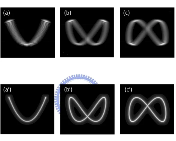
_hω E_{N u u x y N} y x, = + + + + ⎯⎯ →>>1⎯ , ( 1/2) ( 1/2) , (1.4.10)

Figures 1.4.1-1.4.3 depicts the comparison between the quantum wave patterns 2 , , , (ξx,ξy;A,φ) q p u u N _{x y}

Φ and the corresponding classical periodic orbits for p : to be q 2:1,

2 :

3 , and4:3, respectively. Here three different phase factors, φ =0, φ =0.3π , and

π

φ =0.6 , are displayed in each figure for the purpose of clear comparison. The behavior of

the quantum wave patterns in all cases can be found to be in precise agreement with the classical Lissajous figures.

It is worthwhile to mention that the stationary coherent states for the 2D isotropic harmonic oscillator p:q=1:1 can be simplified to give rise to the expression of elliptic states [17]. After some algebra and setting ux =uy =0, equation (1.4.7) can be rewritten as

t N i y x u u N N N y x t C _{x y} A e ω φ ξ ξ ξ ξ 1,1 ( 1) , , 0 ) , ; , ( ) , , ( − + ∞ = Φ = Ψ

∑

, (1.4.11) where

(

)

! 1 2 2 / ) ( 2 2 N e A e C N i y N y y x φ α α + α = − + , (1.4.12)

(

)

∑

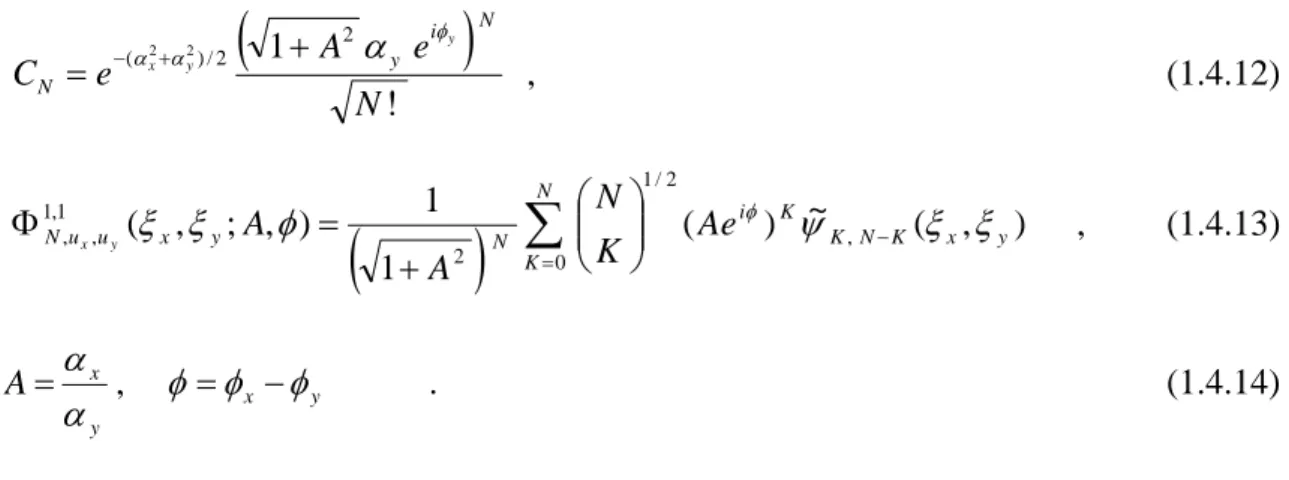
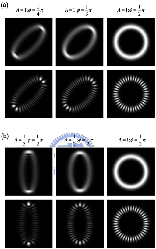
= ⎟⎟⎠ − ⎞ ⎜⎜ ⎝ ⎛ + = Φ N K y x K N K K i N y x u u N Ae K N A A y x 0 , 2 / 1 2 1 , 1 , , ( , ) ~ ) ( 1 1 ) , ; , (ξ ξ φ φ ψ ξ ξ , (1.4.13) y x y x A φ φ φ α α − = = , . (1.4.14)

The wave function in (1.4.13) represents a type of normalized elliptic stationary coherent state. Figure 1.4.4 shows the dependence of the wave pattern of the stationary coherent states

2 1 , 1 0 , 0 , (ξx,ξy;A,φ) N

Φ on the factors A and φ for N=20. It can be seen that the coherent states

) , ; , ( 1 , 1 0 , 0 , ξx ξy Aφ N

Φ correspond to the elliptic stationary states. The superposition of two

elliptic states with a phase factor φ in the opposite sign can form a standing wave pattern: )) , ; , ( ) , ; , ( 1,1_,0,0 1 , 1 0 , 0 , ξ ξ φ ±Φ ξ ξ −φ

Φ_{N x y} A _{N x y} A . Figure 1.4.4 also shows the standing wave

patterns corresponding to the elliptic states.

Equation (1.4.11) manifestly reveals the relationship between the Schrödinger coherent state and the stationary coherent state. As is known from quantum mechanics, C_N 2

represents the probability of finding the system in the elliptic stationary state with order N. With equation (1.4.12), it can be found that

(

)

( ) 2 2 2 2 2 ! y x e N C N y x N α α α α + − + = , (1.4.15)

As the result of the Schrödinger coherent state in the 1D harmonic oscillator, the probability distribution C_N 2 is identical to the Poisson distribution with the mean value of

2 2 y x N >=α +α < .

(a) (b) (c)

(a’)’) (b’) (c’)

(a) (b) (c)

(a’)’) (b’) (c’)

Fig. 1.4.1 Comparison between the quantum stationary state , 2 , , (ξx,ξy;A,φ) q p u u N x y Φ [(a)-(c)] and the classical Lissajous orbits [(a’)-(c’)] for the system of p:q=2:1 with N =40, A=5.2 and (a) φ =0, (b) φ =0.3π , and (c) φ =0.6π .

(a) (b) (c)

(a’)’) (b’) (c’)

(a) (b) (c)

(a’)’) (b’) (c’)

Fig. 1.4.2 The same as Fig. 1.4.1 for the system of p:q=3:2 with N =22, A=5.2 and (a)

0 =

(a) (b) (c)

(a’)’) (b’) (c’)

(a) (b) (c)

(a’)’) (b’) (c’)

Fig. 1.4.3 The same as Fig. 1.4.1 for the system of p:q=4:3 with N =15, A=5.2 and (a)

0 =

π φ 4 1 ; 1 = = A φ π 3 1 ; 1 = = A φ π 2 1 ; 1 = = A π φ 2 1 ; 1 = = A π φ 2 1 ; 2 1 ₌ = A π φ 2 1 ; 3 1 ₌ = A

(a)

(b)

π φ 4 1 ; 1 = = A φ π 3 1 ; 1 = = A φ π 2 1 ; 1 = = A π φ 2 1 ; 1 = = A π φ 2 1 ; 2 1 ₌ = A π φ 2 1 ; 3 1 ₌ = A

(a)

(b)

Fig. 1.4.4 (a) Upper: wave patterns of stationary coherent states for N=20 with different values of the parameters φ. Lower: standing wave patterns corresponding to upper figures. (b) Upper: wave patterns of stationary coherent states for N=20 with different values of the parameters A. Lower: standing wave patterns corresponding to upper figures.

1.5 Unitary Transformation between Stationary States and wave

packet states

Even though the Schrödinger coherent state is an analytic and elegant representation for the wave packet state, another important representation is given by

) ( ) ( ~ 1 ) ; , ( 1 0 N M e e M t M m t E i m N m i m N << = Ψ

∑

− = − + + h ξ ψ φ ξ φ . (1.5.1)

The representation in equation (1.5.1) resembles the definition of the phase state. Unlike the Schrödinger coherent state, the coherent state in equation (1.5.1) is expanded by a finite-dimensional basis. In order to simplify the representation of the wave function, here I use

∑

− = Φ = Ψ 1 0 1 M m m m i n n e M φ (1.5.2)

to replace (1.5.1). The phase φ_n must be properly chosen to make the wave function to maintain the characteristic of orthonormal. Then we can get

( ) s M n M e M ns n s M m m i s n n s = ⇒ = ⋅ = ⋅ = Ψ Ψ

∑

− = −φ _{δ φ} π _φ π φ 2 , 2 1 , 1 0 . (1.5.3)

Continuously, the relation between wave packet states and stationary states can be shown as following: n m M i n m e M π 2 1 = Ψ Φ n m M i m n e M π 2 1 − = Φ Ψ n m M i m n n m M n n n m m e M C C π 2 1 0 1 − − = ⋅ = Φ Ψ = ⇒ Ψ = Φ

∑

. (1.5.4)

Finally, (1.5.5) shows that the stationary states can be represented as the superposition of wave packet states and vice versa.

∑

− = Φ = Ψ 1 0 2 1 M m m n m M i n e M π

∑

∑

∑

− = − = − − = − ⎟⎟ ⎠ ⎞ ⎜⎜ ⎝ ⎛ Φ = Ψ = Φ 1 0 1 0 2 2 1 0 2 1 1 1 M n M m m n m M i n m M i M n n n m M i m e M e M e M π π π . (1.5.5)

It is worthy to notice that iMmn

mn e M U π 2 1

ˆ ₌ is the unitary operator which represents the

transition matrix from the wave packet states and stationary states. Figure 1.5.1 shows the 1D wave packet states (1D Schrödinger coherent states) and stationary states (eigenstates). Figure 1.5.1(a) represents the wave packet states Ψ_n as M =5 and n=0~4 respectively. On the

other, Fig. 1.5.1(b) reconstructs the stationary states from the superposition of wave packet states as M =5 and m=0~4 respectively.

In 1D harmonic oscillator, the unitary transform not only connect the wave packet states and stationary coherent states but also play an important role in the quantum-classical correspondence. To expand the method, the unitary transform of equation (1.5.5) can also express the relation between the time-independent stationary coherent states and eigenstates of 2D harmonic oscillator. Figure 1.5.2 depicts time-independent elliptical stationary coherent states as M =7 and n=0~6 respectively. On the other, Fig. 1.5.3 reconstructs the eigenstates from the superposition of stationary coherent states as M =7 and m=0~6

respectively.

In summary, the wave packet states and stationary states can be constructed by each other with unitary transformation in 1D harmonic oscillator. Therefore, the time-independent stationary coherent states and eigenstates can also be constructed by each other with unitary transformation in 2D harmonic oscillator.

(a)

(b)

(a)

(b)

Fig. 1.5.1 (a) The 1D wave packet states with M =5 and n=0~4 respectively. (b) The 1D stationary states with M =5 and m=0~4 respectively.

(a) (b) (c) (d)

(e) (f) (g) (h)

(a) (b) (c) (d)

(e) (f) (g) (h)

(a) (b) (c) (d)

(e) (f) (g) (h)

(a) (b) (c) (d)

(e) (f) (g) (h)

REFERENCES

[1] Stephen Gasiorowicz, Quantum physics (third ed.), 2003. [2] David J. Griffiths, Introduction to Quantum Mechanics, 1994. [3] http://en.wikipedia.org/wiki/Lissajous_curve

[4] W. Li, L. E. Reichl, and B. Wu, Phys. Rev. E 65, 056220 (2002).

[5] R. Narevich, R. E. Prange, and O. Zaitsev, Phys. Rev. E 62, 2046 (2000). [6] J. Wiersig, Phys. Rev. E 64, 026212 (2001).

[7] J. A. de Sales and J. Florencio, Physica A 290, 101 (2001).

[8] M. Brack and R. K. Bhaduri, Semiclassical Physics (Addison-Wesley, Reading, MA,1997), Sec. 2.7.

[9] F. von Oppen, Phys. Rev. B 50, 17151 (1994). [10] R. W. Robinett, Am. J. Phys. 65, 1167 (1997).

[11] Y. F. Chen, K. F. Huang, and Y. P. Lan, Phys. Rev. E 66, 046215 (2002). [12] Y. F. Chen, K. F. Huang, and Y. P. Lan, Phys. Rev. E 66, 066210 (2002). [13] Y. F. Chen and K. F. Huang, Phys. Rev. E 68, 066207 (2003).

[14] Y. F. Chen and K. F. Huang, J. Phys. A 36, 7751 (2003). [15] E. Schrödinger, Naturwiss. 14, 644 (1926).

[16] Y. F. Chen and Y. P. Lan, PHYSICAL REVIEW A 67, 043814 (2003).

[17] Y. F. Chen, T. H. Lu, K. W. Su, and K. F. Huang, PHYSICAL REVIEW E 72, 056210 (2005).

Chapter 2

Eigenstates of Harmonic Oscillator and

Spherical Laser Cavity:

Generalized Coherent States and Polarization-

entangled Patterns

It is well known that the paraxial wave equation for the spherical resonator has the identical form with the Schrödinger equation for the two dimensional (2D) harmonic oscillator. In this chapter we derive the paraxial wave equation has the same form with the Schrödinger equation for the 2D harmonic oscillator. The wave function for the paraxial field in the spherical laser resonator can be expressed as Hermite-Gaussian (HG) function with Cartesian symmetry or Laguerre-Gaussian function with cylindrical symmetry which are the eigenfunctions of harmonic oscillator mentioned in chapter one. We introduce the generalized coherent states (GCSs) to be related to the transition form HG modes to various experimental modes which are high order polarization-entangled transverse modes. With the connection between theoretical analysis and experimental results, the formation of complicated singularities can be represented.

2.1 Paraxial Approximation of Maxwell’s Equations

According to the Helmholtz wave equation, the wave propagation in a source-free medium follows the Maxwell’s equations which can be represented as [1-2]

0 0 = ⋅ ∇ = ⋅ ∇ ∂ ∂ = × ∇ ∂ ∂ − = × ∇ H E E t H H t E ε µ (2.1.1).

Therefore, the electric field can be expressed as

0 2 2 2 = ∂ ∂ − ∇ E t E µε . (2.1.2)

Assume the electric field to be monochromatic wave E = E

(

x,y,z

)

⋅eiωt, Eq. (2.1.2) can be written as

(

∇2 +k2

)

E

(

x,y,z

)

=0, (2.1.3) where k is the wave vector. For a wave which propagates primarily along the z direction,

(

x y z

)

E

E = , , can be written as

(

x y z

) (

u x y z

)

e ikzz

E , , = , , ⋅ − , (2.1.4)

where u

(

x,y,z

)

is the transverse variation, k_z is the z-component of the wave vector. Substituting Eq. (2.1.4) into Eq. (2.1.3), the Helmholtz equation is represented as

(

)

(

, ,

)

0 2 2 2 2 2 2 2 2 2 = ⎥ ⎦ ⎤ ⎢ ⎣ ⎡ − + ∂ ∂ − ∂ ∂ + ∂ ∂ + ∂ ∂ z y x u k k z ik z y x z z . (2.1.5)

In the paraxial approximation, the term u

(

x y z

)

z2 , ,

2 ∂

∂

is quite small in comparison with remaining terms, therefore

(

, ,

)

0 2 2 2 = ⎥⎦ ⎤ ⎢⎣ ⎡ ₊ ∂ ∂ − ∇ k u x y z z ik_{z t} t , (2.1.6) where 2 2 2 2 2 y x t ∂ ∂ + ∂ ∂ =

∇ and k_t2 =k2 −k_z2. We assume that u

(

x,y,z

)

=Ψ

( ) (

x,y G x,y,z

)

, where Ψ

( )

x,y is a scalar wave function which describes the transverse variation of the beam,

(

x y z

)

G , , is a wave function which describes the wave as Gaussian spherical wave between plane wave and spherical wave. According to the cavity confinement, the Gaussian spherical wave can be written as

(

)

( )

_{( )}

( R( )z ) y x ik z z y x ikz R R _e z e z z z z y x G 2 R 0 2 2 2 2 2 2 2 2 2 , , + − ⎥ ⎥ ⎦ ⎤ ⎢ ⎢ ⎣ ⎡ + + − = + = ω ω , (2.1.7)

where ω0 is the minimum spot size at z =0, ω

( )

z is the spot size at arbitrary position, and

( )

z

R is the radius of curvature. The relation is given by

( )

2 0 1 ⎟⎟ ⎠ ⎞ ⎜⎜ ⎝ ⎛ + = R z z z ω ω and

( )

⎥ ⎥ ⎦ ⎤ ⎢ ⎢ ⎣ ⎡ ⎟ ⎠ ⎞ ⎜ ⎝ ⎛ + = 2 1 z z z z

R R _{. Then Eq. (2.1.6) can be written as}

( ) (

, , ,

)

0 2 2 2 Ψ = ⎥⎦ ⎤ ⎢⎣ ⎡ ₊ ∂ ∂ − ∇ k x y G x y z z ik_{z t} t . (2.1.8)

Using paraxial approximation and after some algebra, the paraxial wave equation can be analyzed as: