類神經網路於結構半主動控制系統之研究(II)

(1)

行政院國家科學委員會專題研究計畫成果報告

類神經網路於結構半主動控制系統之研究

Development of Ar tificial Neur al Networ k Semi-Active Str uctur e Contr ol System

計畫編號：NSC90-2211-E-009-060 執行期限：90 年 08 月 01 日至 91 年 07 月 31 日主持人：洪士林國立交通大學土木工程系 中文摘要 本研究計畫包括兩個部分，第一個部分是以類神經網路控制模式來發展新的最佳化結構半主動控制理論，此網路稱之為可調式半主動神經控制器（Adaptive Neural Structural Semi-Active Controller, ANSSA Controller）。ANSSA Controller 以抵消累積反應的觀念來施加主動可變阻尼力，可以有效地解決時間延遲的問題，並大量地減低結構反應。第二個部分則是設計及製作一可調式的流體阻尼器，藉由改變結構之阻尼值而達到結構控制之目的。 關鍵詞：結構半主動控制、時間延遲、類神經網路、 誤差向後推導學習演算法（BP）、L-BFGS 學習演算法 1. Abstr act

This study includes two parts. The first part presents a neural-network-based semi-active control algorithm, termed Adaptive Neural Structural Semi-Active Controller (ANSSA Controller), to control civil engineering structures under dynamic loading. The ANSSA Controller minimizes structural cumulative responses during earthquakes by applying active variable damper forces. The problem of time delay is considered in the control strategy so that the active variable damper forces can be calculated in time, prepared for, and applied. The ANSSA Controller also circumvents the difficulty of obtaining system parameters of a real structure for the algorithm for structural control. The second part is the design and production of an adaptive fluid damper, which is capable of varying the damping coefficient in a structural control system to suppress structural vibration.

Keywor ds: Structural Semi-Active Control, Time Delay, Error Back-propagation Learning Algorithm, L-BFGS Learning Algorithm

2. Motive and Goal

Semi-active control systems, maintaining the reliability of passive control systems while taking advantage of the adjustable parameter characteristics of an active control system, typically require a small external power source for operation and utilize the motion of the structure to develop the control forces.

Housner et al.1 indicated that the control strategies deemed appropriate for civil engineering structural control should be simple, but robust and fault tolerant; in addition, they do not need to be an optimal control, and must be implemented. Notably,

the artificial neural network (ANN) model is robust and fault tolerant.2-4 In addition, ANN can effectively deal with qualitative, uncertain, and incomplete information. Therefore, ANN is highly promising for structural control. A Number of researchers have developed ANN models for active structural control, including Nikzad and Ghaboussi5, Wen et al.6 and Tang7; besides, Hung et al.8 presented an ANN Controller, Adaptive Neural Structural Active Pulse (ANSAP) Controller, to control civil engineering structures under dynamic loadings. The ANSAP Controller attempts to reduce the structural cumulative responses during earthquakes by applying the active pulse control force. All of the above references show that ANNs are effective for structural active control. However, there is still no published reference about ANN models for structural semi-active control.

The fluid damper9-10 is a promising control system wildly used in mechanical engineering. In the last decade, civil engineers adopt the fluid damper as a dissipater to decrease seismic responses of structures. The characteristic of its energy dissipation is excellent in buildings under strong excitation.

3. Contents of the Resear ch

3.1 Background

Extending the ANSAP Controller, this work presents an ANN control model, Adaptive Neural Structural Semi-Active (ANSSA) Controller, to control civil engineering structures under dynamic loadings. The proposed ANN semi-active control model uses an adaptive L-BFGS ANN learning algorithm27 with a standard BP ANN learning algorithm. The proposed control strategy attempts to reduce the structural cumulative responses during earthquakes by applying the control force generated by active variable damper devices. The ANSSA Controller has three components: (1) a neural emulator network to represent the minimized cumulative structural responses under both the seismic loading and the control force; (2) a neural control network to determine the control force on the structure; and (3) a neural prediction network to predict the future structural response.

3.2 Control Algorithm

The responses of a system with a linear

n-degree-of-freedom structure, when the system is subjected to an external excitation in configuration space, can be described by the following equation

) ( ) ( ) ( ) ( ) (t Cx t Kx t B1u t E1w t x

(2)

where constant matrices M, C, and K are, respectively, the mass, damping, and stiffness matrices with n×n

entities; x(t) is the n-dimensional displacement vector with respect to the ground; u(t) is the p-dimensional control force vector; w(t) is the q-dimensional external excitation vector; and the n×p matrix B1 and n×q

matrix E1 are location matrices that define the

locations of the control force and the excitation, respectively. While assuming that the control force and external excitation are constants in any sampling period

∆

t

, Eq. (1) can be written in a discrete state equation as follows:

[ ]

k 1 Adz[k] Bdu[k] Edw[k] z + = + +

(2)

where t d Ä eA A = , B =A−1(A −I)B d d , and E I A A E = −1( − ) d

d . Index k is an integer number; k =

0, 1, 2, … N; 1 2 1 [ ] 1 [ ] 1 [ ×       + + = + n k k k x x z & is a

2n-dimensional state vector of the structure response at time t = (k+1)

∆

t

, and

∆

t

is the time length of the sampling period. The matrices A, B, and E can be determined by the following:

n 2 n 2 1 1 × − −       − − = C M K M I 0 A ; p n 2 1 1 × −       = B M 0 B ; q n 2 1 1 × −       = E M 0 E (3-5) The main notion of the cumulative response destroying control algorithm is to destroy the gradual rhythmic buildup of the structural response by applying control force of suitable magnitude and proper direction. Thus, the proposed control strategy is to apply the control force to minimize the system response that carries over from the current time step to the next time step. The first two terms in the right-hand side of Eq. (2) represent the structural response that carries over from time k

∆

t

to time (k+1)

t

∆

after the control force u[k] has been applied. That is, the structural response z[k] at any time k

∆

t

should be eliminated by applying a control force u[k].

z*[k]=Adz[k]+Bdu[k]=0

(6)

The control force can be obtained as ] [ ] [ ) ( ] [ T 1 T k k k BdBd BdAdz Gz u =− − =

(7) Considering time delay problem, the control force u[k] has to be computed and prepared before time k

∆

t

, and applied to the structure from time k

∆

t

to time (k+1)

∆

t

. Thus, it’s impossible to calculate u[k] by using z[k]. Assuming that n time step is needed to compute and prepare the control force, the control force can be represented by the following equation: u[k]=g(z[k-n], … , z[k-n-nz], w[k-n], … , w[k-n-nw])

( 8 )

where nz and nw are the maximum lags in the structural response and the external excitation, respectively; and

g is some vector-valued linear or nonlinear function. Consequently, there is time to calculate and prepare the control force from time (k-n)

∆

t

to k

∆

t

and to apply it to the structure from time k

∆

t

to (k+1)

∆

t

.. Thus, the problem of time delay effect can be circumvented in the proposed control strategy.

3.3 ANSSA Controller

For simplicity, assume that only one active tendon controller is used, and that it can be used on any floor. After controlling each degree of freedom, all the relative displacements and relative velocities of the structure cannot be kept at zero by a single control force, but minimizing the cumulative structural responses allows us to apply the single control force. Hence, modifying the control strategy is an attempt to minimize the cumulative structural responses, z*[k] in Eq. (6), by applying the control force. The simplest way to achieve this aim is to minimize the sum of the square of the cumulative structural responses, which happens to be an unconstrained optimization problem, solved most effectively using supervised ANN models.

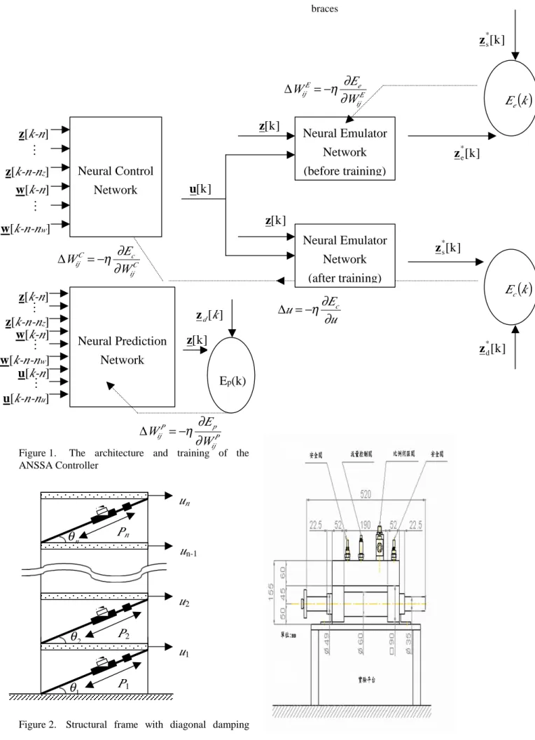
The ANSSA Controller, schematically presented in Fig. 1, consists of three components: (1) a neural emulator network to represent the minimized cumulative structural responses under both the seismic loading and the control force; (2) a neural control network to determine the control force on the structure; and (3) a neural prediction network to predict the future structural response. The details of these three components of the ANSSA Controller are presented in the following.

3.3.1 Neural Emulator Network (NEN)

This network is modeled by an adaptive L-BFGS neural network model11, which models the dynamic behavior of the structure described by Eq. (6). To minimize the sum of the square of the cumulative structural responses, vectors u[k] and z[k] are the inputs, and vector z*[k] is the corresponding output of the neural emulator network. The input data of the training instances are generated randomly, and are substituted into Eq. (6) to generate the desired outputs of the training instances. The computed outputs are then generated by feeding the inputs forwardly through the network. The difference between the desired and computed outputs, z*e[k] and [ ]

* k s

z , of the neural emulator network is then measured. Finally, the weights of the network are adjusted based on the error function Ee(k).

3.3.2 Neural Control Network (NCN)

The neural control network searches a suitable control force to minimize the cumulative structural responses z*[k]. According to Eq. (8), the inputs of the neural control network are z[k-n], … ,z[k-n-nz], w[k-n], … , w[k-n-nw], and the corresponding output is

(3)

u[k]. In this study, a conventional BP neural network is adopted as the neural control network.

Before the neural control network can be trained, the neural emulator network has to be trained. The training process of the neural control network is also demonstrated in Fig. 1. First, presenting the input vector z[k-n], … , z[k-n-zz], w[k-n], … , w[k-n-nw] to the neural control network to compute the control force u[k], that is then applied to the pre-trained neural emulator network to obtain the minimized cumulative response z*s[k]. The error function Ec(k) can be

formulated as follows:

( )

=

_∑∑

P

[

−

]

1 p= 0 o * ps o * pd c k k P k E 2 ] [ ] [ 2 1 z z (9) where P is the number of instances in the training set; and z*pd[k] is the desired minimized cumulative responses of the structure to be controlled, chosen to be zero in this work. The superscript o represents the oth element of the output vectors. Second, the weights

C ij

W in the neural control network are then updated as follows:         ∂ ∂     ∂ ∂ η − = ∆ ∂ ∂ η − = ∆

∑

C ij k k k c C ij C ij c C ij W u u E W W E W ; (10-11) Herein, the learning ratio is a constant. Term uk is the kth component of the control force, u. Eq. (11) indicates that the adjustment of the weight

C ij

W during the training process is split into two steps: first back-propagating the system error function Ec

through the pre-trained neural emulator network without any changes in the weights E

ij

W to calculate the corresponding error u of the control force u; then back-propagating the error

∆

u

through the neural control network to adjust the weights C

ij W . The training process is terminated as the minimized cumulative structural responses converge to the desired responses within the predetermined tolerance. 3.3.3 Neural Prediction Network (NPN)

The obvious equation for n-step structural response prediction can be expressed as

]) [ ] [ ] [ ] [ ] [ ] [ ( ] [ u w z n -n -k , , n -k , n -n -k , , n -k , n -n -k , , n -k h k u u w w z z z L L L =

(12) where nz, nw and nu are the maximum lags in the structural response, the external excitation and the control force, respectively; and h is some vector-valued linear or nonlinear function.

Function h in Eq. (12) can be approximated by the ANN, called Neural Prediction Network (NPN), as shown in Fig. 1. The inputs of the NPN are structural responses z[k-n], … , z[k-n-nz], external excitations w[k-n], … , w[k-n-nw], and control forces u[k-n], … , u[k-n-nu]. The output of the NPN is the structural response in the kth time step, z[k]. Herein, the NPN is

implemented through an adaptive L-BFGS neural network model.

3.4 Adjusting the Damping Coefficient of the Active Variable Dampers

After the ANSSA Controller has been trained, the damping coefficient of the active variable dampers can be adjusted according to the outputs of the NCN and NPN. Assuming that the active variable dampers are installed in parallel along diagonal braces that are hinged to the main structure as shown in Fig. 2.

Let F[k]=du[k] (13) where n n×                 ⋅⋅ ⋅ ⋅⋅ ⋅ ⋅⋅ ⋅ ⋅⋅ ⋅ ⋅⋅ ⋅ ⋅⋅ ⋅ = 1 1 1 1 1 1 1 1 1 d

(14) F[k]=[F1[k] F2[k] … Fi[k] … Fn[k]]T is the vector of

the control forces (at time k

∆

t

) produced by the active variable dampers; Fi[k] is the control force (at time k

∆

t

) produced by the active variable dampers installed between the i-th and (i-1)-th floors; u[k]=[u1[k] u2[k] … ui[k] … un[k]]T is the control

force vector (at time k

∆

t

) calculated by the NCN; and

ui[k] is the control force (at time k

∆

t

) of the i-th floor. The active variable damper forces can be expressed as

Fi[k]=-Pi[k]cos i (15)

where Pi[k] is the active variable damper force (at time

k

∆

t

) between the i-th and (i-1)-th floors; and i is

the angle of inclination of the dampers installed between the i-th and (i-1)-th floors. The active variable damper force also can be expressed as

( )

[ ]

( )

SAi

(

i

[ ]

i

[ ]

)

i i i i SA i i k x k x C N k v C N P θ − = θ = − cos cos 1 i & & (16-17) where Ni is the number of dampers installed between the i-th and (i-1)-th floors; vi[k] is the internal velocity (at time k

∆

t

) of the dampers installed between the

i-th and (i-1)-th floors; x&i

[ ]

k is the relative velocity

(at time k

∆

t

) of the i-th floor predicted by NPN; and (CSA)i[k] is the damping coefficient (at time k

∆

t

) of

the dampers installed between the i-th and (i-1)-th floors. Thus, the adjustment in the damping coefficient of each active variable damper is given by

( )

[ ]

( )

[ ]

( )

[ ]

( )

     ≥ ≤ ≤ ≤ = C C C C k C C k C C C C k C max * i SA max max * i SA min * i SA min * i SA min i SA if if if (18) where

( )

[ ]

₍

_{[ ]}

[ ]

_{[ ]}

₎

i i i i i * i SA k x k x N k F k C θ − − = − 2 1 cos & & (19)

(4)

3.5 The numerical examples

SDOF and MDOF structural systems subjected to EL-Centro, Hachinohe and Myiagiok earthquake, were investigated to demonstrate the feasibility of the ANSSA Controller. Results indicate that the proposed semi-active control algorithm destroys the gradual rhythmic buildup of the structural response and reduces the structural responses significantly at the peak of the relative displacement, velocity, and acceleration.

4. Adaptive Fluid damper

In order to verify the control algorithm, an adaptive fluid damper is designed and experimented. Figure 3 shows the adaptive fluid damper used in this study. The damper consists of a stainless steel piston, safe valve, flow control valve, and proportional servo valve.. Experimental results indicate that the adaptive fluid damper can enhance the energy absorption of a structure during earthquakes. The damping coefficient of the damper can be adapted via adjusting the propositional valve to perform variant energy absorption capacity. The experiment results reveal that the adaptive fluid damper

5. Comment and Conclusion

In this work, we present a semi-active control algorithm using ANN model, called Adaptive Neural Structural Semi-Active Controller (ANSSA Controller), to control civil engineering structures under dynamic loadings. The control strategy of the ANSSA Controller aims to minimize the structural cumulative responses during earthquakes by applying the active variable damper forces; besides, the problem of time delay is considered in the proposed control strategy.

6. Refer ences

[1] G. W. Housner, T. T. Soong and S. F. Masri,. ‘Second generation of active structural control in civil engineering, final program and abstracts’, In:

First World Conf. on Structural Control, 3-5 August, Los Angeles, CA (1994).

[2] H. Adeli and S. L. Hung, Machine Learning – Neural networks, Genetic Algorithms, and Fuzzy Systems, John Wiley & Sons, New York, 1995. [3] A. K. Johan, P. L. Joos, and L. R. Bart, Artificial

Neural Networks for Modeling and Control of Non-Linear Systems, Kluwer Academic Publishers, Boston, 1996.

[4] D. E. Rumelhart, G. E. Hinton, and R. J. Williams, ‘Learning international representation by error propagation’, In Parallel Distributed Processing, Rumelhart, D. E. et al., eds., The MIT Press, Cambridge, MA, 318-362 (1986). [5] K. Nikzad and J. Ghaboussi, ‘Application of

Multi-Layered Feedforward Neural Networks in Digital Vibration Control’, Proc. International

Joint Conference on Neural Networks, Seattle, WA, II A-1004 (1991).

[6] Y. K. Wen, J. Ghaboussi, P. Venini and K. Nikzad, ‘Control of structures using neural networks’, In: Proc. of US/Italy/Japan Workshop on struct. control and intelligent systems, Sorrento, Italy, 232-251 (1992).

[7] Y. Tang, ‘Active control of SDF systems using artificial neural networks’, Comp. and Struct., 60(5), 695-673 (1995).

[8] S. L. Hung, C. Y. Kao and J. C. Lee, ‘Active Pulse Structural Control Using Artificial Neural Network’, J. Engrg. Mech., ASCE, 126(8), 839-849 (2000).

[9] M. D. Symans and M. C. Constantinou, ‘Semi-active control systems for seismic protection of structures: a state-of-art review’,

Enginreering Structures, 21, 469-487 (1999). [10] M. D. Symans and M. C. Constantinou, ‘Seismic

testing of a building structure with a semi-active fluid damper control system’, Earthquake Engrg. Struct. Dyn., 26, 759-777 (1997).

[11] S. L. Hung and Y. L. Lin, ‘Application of an L-BFGS neural network learning algorithm in engineering analysis and design’, Proc., 2nd Nat. Conf. on Struct. Engrg., Chinese Soc. of Struct. Engrg., Nantou, Taiwan, R.O.C. , 221-230 (1994).