無線感測網路中行動感測器派遣演算法

國

立

交

通

大

學

資訊科學與工程研究所

碩

士

論

文

無線感測網路中行動感測器派遣演算法

Energy-Efficient Algorithms for Dispatching Mobile Sensors

in a Wireless Sensor Network

研 究 生：張民憲

指導教授：彭文志 教授

無線感測網路中行動感測器派遣演算法

Energy-Efficient Algorithms for Dispatching Mobile Sensors in a Wireless Sensor Network

研 究 生：張民憲 Student：Min-Hsien Chang

指導教授：彭文志 Advisor：Wen-Chih Peng

國 立 交 通 大 學

資 訊 科 學 與 工 程 研 究 所

碩 士 論 文

Submitted to Institute of Computer Science and Engineering

College of Computer Science

National Chiao Tung University

in partial Fulfillment of the Requirements

for the Degree of

Master

in

Computer Science

June 2006

Hsinchu, Taiwan, Republic of China

無線感測網路中行動感測器派遣演算法

學生：張民憲

指導教授：彭文志

國立交通大學資訊科學與工程研究所碩士班

摘 要

在一混合式之無線感測網路中，固定式感測器負責偵測事件的發生，

而行動感測器可以移動至事件發生點以便作進一步分析。行動感測器最耗

能的操作即為移動，如何減少感測器之移動距離同時能讓其完成任務為一

富有挑戰性之研究題目。若某些特定行動感測器一直被指派到不同的地

點，他們的能量很快就會耗盡，並造成殘存感測器之工作負擔變大。在平

衡各感測器之工作負擔的前提之下，本論文提出一有效派遣行動感測器之

演算法，並且適用於任意數量之可動式感測器以及事件發生點。行動感測

器的數量大於事件發生點時，本論文將其轉化為一最大配對數之配對問題

(maximum matching problem)，而在事件發生點大於感測器的數量時，我

們將事件先叢集化，並將行動感測器分配到各叢集完成任務。為了減少感

測器之間的訊息傳輸量，本論文提出一分散式演算法。模擬實驗結果證明

本 論 文 所 提 出 之 演 算 法 能 夠 有 效 的 延 長 行 動 感 測 器 之 系 統 生 命 週 期

(system lifetime)。

Energy-Efficient Algorithms for Dispatching Mobile Sensors in a Wireless

Sensor Network

Student：Min-Hsien Chang Advisor：Dr. Wen-Chih Peng

Institute of Computer Science

National Chiao Tung University

ABSTRACT

A hybrid sensor network consists of both static and mobile sensors, where the

former is used to detect events while the latter can move to event locations for

conducting more advanced analysis. By exploring the load balance of mobile

sensors, we propose an algorithm CentralSD to efficiently dispatch mobile

sensors. Our algorithm is general in which the numbers of mobile sensors and

events are arbitrary. When the number of events is no larger than that of mobile

sensors, we transform the dispatch problem to a maximum matching problem in

a weighted bipartite graph. When there are only few mobile sensors to be

dispatched to a large number of event locations, we propose an efficient

clustering scheme to group event locations so that the maximum matching

approach can be applied. To reduce messages incurred, we also develop a

distributed algorithm GridSD. Extensive simulation results are presented to

verify the effectiveness of our proposed algorithms.

誌 謝

漫漫長路，這篇能夠呈獻出我這兩年來研究成果的碩士論文終於問世，

在研究所的這段日子裡，有太多人與事都值得感謝，回憶起那些奮鬥到天

明，掙扎著從實驗室騎摩托車回到宿舍馬上倒地不起的日子，現在倒是能

夠微微地揚起嘴角懷念著那努力的過程。

首先要感謝指導教授彭文志老師，老師順利的引領我轉換到本論文的

題目，並且在這個題目裡給我很多指導以及建議，如此才能有這篇論文的

誕生。還需要感謝王友群學長在論文後期給予我的指正以及幫助，讓我對

於自己的題目能有更深入且多面向的理解，洪智傑學長提供了我許多對於

數學證明以及表示法的建議，而且常常充滿活力的鼓舞我們一度低迷的士

氣。

實驗室的革命同志們：慧友、志劭以及向彥，有了你們各種方式的鼓

勵與幫助我才能夠順利完成論文，回憶起大家一起吃飯一起打嘴炮的日

子，讓我更能堅定的往人生的下段旅程前進，實驗室的各位學弟妹也提供

我更廣闊的思維以及生活經驗。

最後我將感謝我的家人，在新竹的姊姊常常把我拉去吃飯，讓我免於

吃泡麵過活的日子，在台中家裡的奶奶和爸媽的支持讓我全心全意投入本

篇論文，你們的支持與鼓勵是本篇論文最重要的推手。感謝你們!

目

錄

頁次

中文摘要

………

I

英文摘要

………

II

誌謝

………

III

目錄

………

IV

圖目錄

………

V

1、

Introduction……… 1

2、

The Sensor Dispatching Problem………

8

3、

Algorithms for Dispatching Mobile Sensors………

11

3.1

Algorithm CentralSD：A Centralized Dispatch Method…

11

3.1.1 Case of |S| ≥ |L| ………

11

3.1.2 Case of |S| < |L| ……… 17

3.2

Algorithm GridSD：A Distributed Dispatch Method ………

20

4、

Experimental Results ………

25

4.1

Effectiveness of CentralSD and GridSD ………

25

4.2

The Impact of Load-Balance ………

26

4.3

The Impact of Clustering ………

29

4.4

Sensitivity Analysis on the Coefficient δ……… 29

4.5

Effect of Grid Size α and Search Length β……… 31

5、

Conclusions……… 33

Bibliography

34

圖 目 錄

Figure 1.1: Comparison of different dispatch methods. ………3

Figure 3.1: An example to show how PairMatching works. ………16

Figure 3.2: An example to cluster event locations. ………19

Figure 3.3: An example to show how GridSD works. ………24

Figure 4.1: Comparison on system lifetime. ………27

Figure 4.2: Comparisons on energy consumption. ………28

Figure 4.3: Comparison on number of packet delivery. ………29

Figure 4.4: The effect of clustering on energy consumption. ………30

Figure 4.5: The effect of coefficient δ on redundant iterations and energy

consumption………30

Figure 4.6: The effects of grid size α and search length β on the number of

packet delivery and the discover ratio………32

Chapter 1

Introduction

Recent advances in micro-sensing MEMS and wireless communication technologies have promoted the development of wireless sensor networks (WSN). A WSN has many attractive characteristics including context-aware capability and fast ad-hoc networking con guration, so that it can be widely used in various applications such as border detection, environment monitoring, smart home, and surveillance. However, sensor nodes in a WSN are usually assumed to be simple and prone to error [1]. They may provide rough descriptions of events and even false information when sensors are broken. For example, in a military application, sensors that can detect the change of pressure may be deployed along the borders to determine if an enemy passes. However, these sensors can only report something passing but cannot describe what passes through them. Moreover, failure sensors or incorrect sensing reports will generate false alarms. In this case, we may prefer using more powerful but expensive sensors like cameras to recognize the passing object or to determine whether this is a false alarm. However, it is impossible to mount a camera on each sensor node due to their large number. An alternative and better way is to mount the expensive sensors on few mobile platforms [6, 11, 16], and then dispatch these mobile sensors to visit event locations when necessary. In this paper, we consider a hybrid WSN consisting of static and mobile sensors. The static sen-sors are deployed to detect events, while the mobile sensen-sors equipped with more resources such as sensing capability and computation power are dispatched to these event locations to conduct more

advanced analysis. Since mobile sensors use small batteries for their operations without any addi-tional power source, one important issue of mobile sensors is to conserve their energies. In general, for a mobile sensor, the energy consumption of movement is larger than that of other operations such as sensing, computing and communication. The moving energy cost will be the dominated factor of the energy consumption of a mobile sensor. Therefore, in this paper, we investigate how to ef ciently dispatch mobile sensors to visit event locations with the purpose of maximizing the system lifetime, which is de ned as the time duration until there are some event locations that cannot be reached by any mobile sensor due to lack of energy.

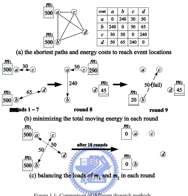
As mentioned above, the problem we shall deal with is to dispatch mobile sensors in an energy-ef cient manner so as to prolong the system lifetime. However, simply optimizing the solution in each one-round dispatch cannot guarantee to maximize the system lifetime. Speci cally, we schedule each mobile sensor to visit certain of event locations in a way such that the total moving energy is minimized. Such procedure is repeated in each round until we cannot nd any mobile sensor with enough energy to reach some event locations. Unfortunately, this iteratively-optimized method may cause some mobile sensors early to exhaust their energies, thereby reducing the system lifetime. Consider an illustrative example in Fig. 1.1, where there are two mobile sensors m1 and

m2 at locations a and b, respectively. Both mobile sensors have an initial energy of 500 units. We

consider only the energy consumption due to movement. Assume that two events occur at locations cand d (resp., a and b) during each odd (resp., even) round. Fig. 1.1(b) shows the execution of the above iteratively-optimized method. To minimize the total moving energy, m1and m2 are assigned

to move between the pair of locations (a; c) and (b; d), respectively, which results in a minimum cost of 95 units in each round. However, after seven rounds, m2 almost runs out of its energy and

has to stay at location d. As a result, m1 should visit both event locations a and b and thus remains

20 units of energy in the eighth round. Finally, in the ninth round, no mobile sensor has enough energy to reach the event location c so that the system lifetime is eight rounds. In fact, when it comes to dispatching mobile sensors, we should not only attempt to reduce the total moving energy

Figure 1.1: Comparison of different dispatch methods.

but also balance the loads of mobile sensors. Fig. 1.1(c) illustrates the above method, where m1

and m2 are assigned to move between the pair of locations (a; d) and (b; c), respectively, resulting

in a slightly higher cost (i.e., 100 units) in each round. Although spending more energy compared with the iteratively-optimized method in each round, the above method indeed extends the system lifetime (i.e., ten rounds). From Fig. 1.1, we can observe that simply optimizing the solution in each one-round dispatch could shorten the system lifetime because the early-exhausted mobile sensors will burden other still alive ones, which in turn early exhausts energy of alive mobile sensors. As the number of early-exhausted mobile sensors increases, the system lifetime will be shortened.

Consequently, in this paper, by balancing the loads of mobile sensors, we propose an algo-rithm CentralSD (standing for Centralized Sensor Dispatching) to dispatch mobile sensors with the

purpose of maximizing the system lifetime. Assume that one central server is available to collect location of mobile sensors and events. In CentralSD, during each round of dispatching, we will determine which mobile sensors should visit which event locations with the objective of minimizing the moving distance (or maximizing the remaining energy) of mobile sensors. However, instead of simply optimizing the objective of dispatching, we exploit the load balance of mobile sensors, in terms of moving distance or remaining energy, during each round. Furthermore, balancing the loads of moving distance also implies that mobile sensors have similar energy costs and moving time to visit event locations, while balancing the loads of remaining energy can avoid a mobile sensor with less energy being dispatched to a long-distance event location. In CentralSD, a more general solu-tion to the sensor dispatch problem is proposed in which the numbers of mobile sensors and event locations are arbitrary. In particular, two cases are considered in CentralSD. Explicitly, when the number of event locations is no larger than that of mobile sensors, we transform the dispatch prob-lem to a maximum matching probprob-lem in a weighted bipartite graph, where the vertex set contains all mobile sensors and all event locations and the edge set contains the edge from each mobile sensor to each event location. However, instead of nding the matching with a minimum edge weight [12], we use a preference list and a bound to select the matching. Speci cally, the preference list helps assign an event location with a suitable mobile sensor, while the bound is to avoid selecting edges with extreme weights so that the load-balance can be achieved. When the number of event locations is larger than that of mobile sensors, we propose an ef cient clustering scheme to group event lo-cations into clusters, where the number of clusters will be the same as that of mobile sensors. In this way, we can adopt the aforementioned matching approach to dispatch each mobile sensor to a cluster of event locations. Then the mobile sensor can use the traveling-salesman approximation algorithm [3] to reach all event locations in that cluster. However, as mentioned above, CentralSD requires a central server to collect information of mobile sensors and events, which incurs a con-siderable amount of message transmissions. To reduce messages incurred, we develop an algorithm GridSD (standing for Grid-based architecture for Sensor Dispatching) to dispatch mobile sensors in

a distributed manner. A comprehensive performance study is conducted and simulation results show that by exploring the load balancing of mobile sensors, our proposed algorithms can have more alive mobile sensors, thereby prolonging the system lifetime.

A signi cant amount of research [2, 8, 19, 20, 21] has elaborated on the issue of using mobile sensors to enhance the sensing coverage or the network connectivity in a WSN. We mention in passing that the authors in [5] considers how to move more sensors close to the locations of events predicted, while still maintaining complete coverage of the sensing eld. However, the concept of sensor dispatch is still not addressed. The authors in [14] exploit the use of mobile sensors to track a moving object with mobile sensors. It is assumed that the object's trajectory can be predicted and the work discusses how to maneuver the mobile sensors to optimally acquire data from the object in real-time. However, the energy consumption of mobile sensors is not considered in [14]. Several research efforts [17, 18] have addressed how to select and move mobile sensors in a hybrid WSN. In [17], static sensors that detect events will invite and navigate nearby mobile sensors to move to their locations. The mobile sensor that have shorter moving distance and more energy, and whose leaving does not cause a large coverage hole, will be invited by the static sensors. In [18], static sensors estimate the coverage holes close to them and use the hole size to compete for mobile sensors. The mobile sensor then selects the largest one and moves to ll that coverage hole. To the best of our knowledge, the attention of prior works was mainly paid to the use of mobile sensors for coverage holes and object tracking, but not to the general dispatch problem explored in this paper.

In this work, we consider how to ef ciently dispatch mobile sensors so that the system lifetime can be extended. In particular, during each one-round dispatch, we will schedule mobile sensors to visit event locations so that the moving distance or the remaining energy of mobile sensors can be minimized or maximized, respectively. However, instead of simply optimizing the solution, we consider to balance the loads of mobile sensors, in terms of moving distance or remaining energy, during each round. By balancing the loads can make each mobile sensor live longer, and thus can help prolong the system lifetime. In addition, balancing the loads of moving distance can make

mobile sensors have similar energy costs and moving time to visit event locations, while balancing the loads of remaining energy can avoid a mobile sensor with less energy being dispatched to a long-distance event location. In this work, we consider a more general solution to the sensor dispatch problem in which we do not restrict the numbers of mobile sensors and event locations. When the number of event locations is no larger than that of mobile sensors, we translate the dispatch problem to the problem of nding a maximum matching in a weighted bipartite graph, where the vertex set contains both the sets of mobile sensors and event locations, and the edge weights can be either the moving distance or the remaining energy, depending on the objective function being used. However, instead of nding the matching with a maximum or minimum edge weight [12], we use a preference list and a bound to select the matching. Speci cally, the preference list can help each mobile sensor select a suitable event location so that it can have a shorter moving distance or remain more energy after movement, while the bound is to avoid selecting edges with extreme weights so that the load-balance can be achieved. When the number of event locations is larger than that of mobile sensors, we propose an ef cient clustering mechanism to group event locations into clusters, where the number of clusters will be the same as that of mobile sensors. In this way, we can adopt the aforementioned solution to dispatch mobile sensors to the clusters of event locations. After we assign a mobile sensor to visit a cluster, it can use the traveling-salesman approximation algorithm [3] to reach all event locations in that cluster. Finally, we have also developed a distributed method based on the aforementioned dispatch solution to avoid the need of a centralized server when dispatching mobile sensors. In summary, our work has the following contributions:

1. We have addressed the importance of load-balance when dispatching mobile sensors and then propose a novel dispatch solution to prolong the system lifetime by balancing the loads of mobile sensors in terms of moving distance and remaining energy.

2. We have proposed an ef cient clustering mechanism to group event locations so that our dis-patch solution can be also suitably applied to the case when there are few mobile sensors that

have to be dispatched to a large number of event locations.

3. We have proposed a distributed version of our dispatch solution so that there is no need of a centralized server to execute our dispatch solution.

It is worth mentioning that we not only explore load-balancing in dispatching mobile sensors, but also develop one clustering mechanism to deal with the case that the number of event locations is larger than that of mobile sensors. These features distinguish this paper from others.

The rest of this paper is organized as follows. In Chapter 2, we formally de ne the sensor dispatch problem. Chapter 3 proposes our solutions to this problem. Simulation results are presented in Chapter 4. Chapter 5 concludes this paper.

Chapter 2

Sensor Dispatch Problem

We consider a hybrid WSN comprised of both static and mobile sensors. Static sensors can form a connected network and fully cover the area of interest to continuously monitor the environment. When events are detected by static sensors, there is a set of n mobile sensors S = fs1; s2; : : : ; sng,

which are randomly distributed over the sensing region and can be dispatched to the event locations (as reported by static sensors) to provide higher quality of sensing results. To achieve this goal, we assume that sensors know their own locations, which can be achieved by the global positioning system (GPS) [9] or other localization techniques [4, 10].

The sensor dispatch problem is modeled as follows. We assume that there is a set of event loca-tions L = fl1; l2; : : : ; lmg, each to be visited by a mobile sensor. We allow an arbitrary relationship

between the values of m and n. The goal is to compute a dispatch schedule SCHsi for each mobile

sensor si such that each location in L is visited exactly once by one mobile sensor. Each schedule

SCHsi is denoted by a sequence of event locations, and the jth location to be visited is written as

SCHsi[j]. Let ei be the current energy of si and c(SCHsi)be the energy required to complete si's

visit schedule,

c(SCHsi) = move (d(si; SCHsi[1])+

jSCH_Xsij 1

j=1

where move is the energy required to move a sensor one-unit distance, d(si; SCHsi[1]) is the

Euclidean distance from si's current location to SCHsi[1], and d(SCHsi[j]; SCHsi[j + 1]) is the

Euclidean distance between SCHsi[j]and SCHsi[j + 1]. Clearly, the schedule must satisfy ei

c(SCHsi).

For performance reason, we de ne two objective functions for the sensor dispatch problem. The rst one is to minimize the total energy consumption to move sensors, i.e.,

minX

si2S

c(SCHsi): (2.1)

The second one is to maximize the total remaining energy of mobile sensors after movement, i.e., maxX

si2S

(ei c(SCHsi)): (2.2)

To balance the energy consumption of mobile sensors, we will also measure the standard deviations of sensors' energy consumption and remaining energies. When we assign the dispatching schedules of mobile sensors in each round. However, as mentioned in Chapter 1, we should also balance the loads of mobile sensors. In this work, we use the standard deviation to measure how balance a dispatching method can achieve. In particular, the standard deviation of the energy consumption among mobile sensors is

1 n X si2S (cavg c(SCHsi)) 2 !1 2 ; (2.3) and the standard derivation of the remaining energy among mobile sensors is

1 n X si2S (eavg (esi c(SCHsi))) 2 !1 2 ; (2.4) where cavg and eavg are the average of the total energy consumption and the total remaining energy

of mobile sensors, respectively. To balance the loads of mobile sensors, we should also minimize either Eq. (2.3) or Eq. (2.4) when assigning their dispatching schedules, depending on the objective function Eq. (2.1) or Eq. (2.2) that we adopt in each round, respectively.

Note that the above modeling is only concerned about one round of sensors' dispatch schedules. In general, multiple rounds of dispatch schedules need to be determined, where each round contains

those events being detected over a xed amount of time, and the goal is to extend mobile sensors' lifetimes to the maximum number of rounds. The length of a round depends on users' real-time constraint. Since event locations are unexpected, we will only focus on the optimization of one round in our work.

Chapter 3

Algorithms for Dispatching Mobile Sensors

We rst propose a centralized solution, where there is a central server which will collect the sets L and S and compute sensors' schedules. Then, a distributed solution will be developed.

3.1 Algorithm CentralSD: A Centralized Dispatch Method

3.1.1 Case of jSj

jLj

For each mobile sensor si 2 S, we rst determine the energy cost c(si; lj)to move si to each event

location lj 2 L. We de ne a cost function c(si; lj) = move d(si; lj). We then construct a weighted

complete bipartite graph G = (S [ L; S L)such that the vertex set contains all mobile sensors and all event locations and the edge set contains the edge (si; lj)from each si 2 S to each lj 2 L.

The weight of (si; lj)is de ned as

if Eq. (2.1) is the objective function, or as w(si; lj) = 8 > > < > > : emax (esi c(si; lj)); if esi c(si; lj) 0; otherwise ;

if Eq. (2.2) is the objective function, where emax is a large value no less than maxsi2Sfesig. For

simplicity, we can set emax = maxsi2Sfesig. It is not hard to see that the objective functions Eqs.

(2.1) and (2.2) can both be reduced to the same goal of minimizing the total weight of a matching. Therefore, with G, our goal is to nd a matching P such that (1) the number of matches in P is the largest, (2) the total edge weight of P is minimized, and (3) the standard deviation of edge weights of P is minimized.

To nd P , we rst associate a preference list P list(si)to each si, which ranks each event location

lj 2 L by its weight w(si; lj)in an increasing order. When edge weights are equal, events' IDs are

used to break the tie. Similarly, for each lj, we associate it with a preference list P list(lj), which

ranks each si 2 S by its weight w(si; lj)in an increasing order.

To reduce the standard deviation of the matching P , we introduce a bound Blj for each lj 2 L

to restrict the candidate mobile sensors with which ljcan match. Speci cally, lj can only consider a

mobile sensor si such that w(si; lj) Blj.

To nd P , we set the initial value of each Blj to the average of the minimum of the weights of

all edges incident to each event location, i.e., Bl1 = = Blm =

Pm

j=1min(si;lj)2S Lfw(si; lj)g

m :

Then, for each lj 2 L, we try to nd a match si 2 P list(lj)with lj such that w(si; lj)is minimized

and w(si; lj) Blj. If we cannot nd such si, we will continue extending Blj with an increasing

level B until lj can nd available mobile sensors. Note that the value of B should be carefully

designed so that the weight of each pair will not increase sharply while the number of extending the bound operations for the next available mobile sensor can be reduced. In view of the above design guide, for each event, we should derive the distance interval of the farthest mobile sensor

and the nearest mobile sensor. Those mobile sensors staying in the distance interval should be taken into consideration for dispatching. Furthermore, when more mobile sensors are given, an event can easily nd a mobile sensor in its neighborhood. Otherwise, one should use larger increasing level to increase the possibility of nding available mobile sensors. Therefore, the increasing level, denoted as B, is formulated as follows: B = mn ( m X j=1 max (si;lj)2S Lfw(s i; lj)g m X j=1 min (si;lj)2S Lfw(s i; lj)g); (3.1)

where is an adjustable coef cient B.

As an unmatched event location lj expands its bound Blj, more candidates will be included in

its P list(lj). If the rst unvisited candidate si in P list(lj) is also unmatched, the pair (si; lj) is

added into P . Otherwise, simust be matched with another event location (e.g., lo). From the bounds

Blj and Blo, we can determine which event location si should be matched. This is referred to as

a competition between lj and lo. In particular, si is matched to lj if one of the following cases is

satis ed.

1. Blj > Blo. Since enlarging the bound will increase the risk of including an edge with an

extreme weight into P , we will prefer matching siwith lj to avoid expanding the larger bound

Blj.

2. Blj = Blo and lj is prior to lo in si's preference list. As si prefers lj to lo, we thus match si

with lj to reduce the total weight of P .

3. Blj = Blo and si is the last candidate in P list(lj)but not in P list(lo). Since lj cannot have

another candidate to pick in P list(lj), sishould be matched with lj.

Once siis matched with lj, the pair (si; lo)should be replaced by the new pair (si; lj)in P , and

lo should search for another mobile sensor to match with. It is possible that lo will compete with

Procedure 1 PairMatching(L; S)

Input: sets of event locations L and mobile sensors S Output: maximum matching P between L and S

1: construct a weighted bipartite graph G = (S [ L; S L); 2: generate a preference list P list(k) for each k 2 fS [ Lg; 3: assign an initial value for each bound Blj;

4: for each lj 2 L that is not matched do

5: while P list(lj)contains no unvisited candidate do

6: Blj = Blj+ B;

7: end while

8: let si 2 S be the rst unvisited candidate in P list(lj);

9: if siis unmatched then

10: add the pair (si; lj)to P ;

11: else

12: let lo 2 L be the location originally matched with si;

13: if Blj > Blo then

14: replace (si; lo)by (si; lj)in P ;

15: else if Blj = Blo then

16: if lj is prior to lo in P list(si)then

17: replace (si; lo)by (si; lj);

18: else if si is the last candidate in P list(lj)but not

in P list(lo)then

19: replace (si; lo)by (si; lj)in P ;

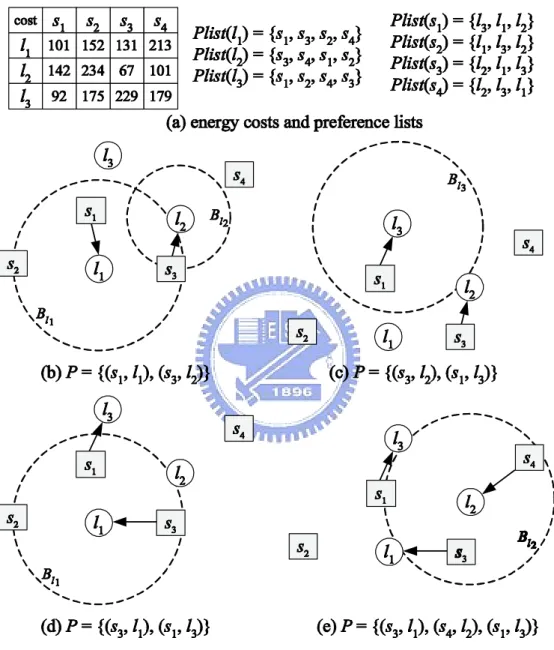
Consider an illustrative example in Fig. 3.1 , where is set to 2. The initial bound is 101+77+92 3 =

90 and the increasing level B =

(213+234+229) (101+77+92)

4 3 2 = 67:7. We start with the event

location l1. Since there is no available mobile sensor in P list(l1)with the initial bound, Bl1 will be

expanded by B. Accordingly, Bl1 is updated to 90+67.7=157.7. As a result, we will have three

candidates (i.e., s1, s2, and s3). Since l1 nds that the rst unvisited candidate s1 is unmatched,

we add (s1; l1) to the matching P . Following the same operation, the pair (s3; l2) is determined,

as shown in Fig. 3.1(b). However, after expanding Bl3, l3 nds that the rst candidate s1 has been

matched with l1. Therefore, l3 will compete with l1 for s1. It can be veri ed that case 2 is satis ed

(i.e., Bl3 = Bl1 = 157:7 and l3 is prior to l1 in P list(s1)). Consequently, (s1; l1) is replaced by

(s1; l3)in Fig. 3.1(c). Following the same procedure, l1will obtain s3 from l2 and then l2 has to nd

an unmatched mobile sensor s4to pair with. Fig. 3.1(e) shows the nal result.

In the above example, we follow the sequence of l1, l2, and l3 to decide the matching. Note that

due to the competition of event locations, the PairMatching procedure can generate the same result no matter what processing sequence we use. This will be proved in Theorem 1. Theorem 2 analyzes the time complexity of PairMatching.

Theorem 1. The result of PairMatching is irrelevant to the processing sequence of event locations. Proof. Suppose that PairMatching generates two different matchings P and P0_{when different}

process-ing sequences are used. Then there must be an event location lx 2 L matched with different

mobile sensors sa and sb in P and P0, respectively. Without loss of generality, we assume that

w(lx; sb) < w(lx; sa), so sb will be prior to sa in P list(lx). In the matching P , since lx has

been matched with sa, sb must be matched with another event location (e.g., ly). Thus, we have

f(lx; sa); (ly; sb)g P. Recall the three cases that ly can win the competition to get sb. Then exactly

one of the following two conditions must be satis ed:

1. ly has the advantage over lx because either Bly > Blx (i.e., case 1) or sb is the last candidate

2. lyis prior to lxin P list(sb)(i.e., case 2).

However, in the matching P0_{, since s}

b is matched with lx, ly will be matched with another mobile

sensor (e.g., sc). As such, we have f(lx; sb); (ly; sc)g P0. In this case, if the rst condition is

satis ed, a contradiction will be occurred because lymust be also matched with scin the matching P .

If the second condition is satis ed, we have Blx = Bly. However, since ly is prior to lxin P list(sb),

sb must be matched with ly rather than with lx in P0, which also causes a contradiction. Therefore,

the result of PairMatching is unique, no matter what processing sequence of event locations we use.

Theorem 2. The time complexity of PairMatching is O(mn lg mn).

Proof. In PairMatching, we rst construct the graph G, which takes O(mn) time since we have to assign the weight of each edge. Then generating the preference lists for all elements in S [ L needs O(mn lg n + nm lg m)time since we have to sort the elements in S and L. The worst case for an event location to nd its matched mobile sensor is O(n) since it has to go through its preference list. Thus, the time to compute the maximum matching P will be O(mn). Therefore, the total time complexity of PairMatching is O(mn + mn lg n + nm lg m + mn) = O(mn lg mn).

3.1.2 Case of jSj < jLj

When the number of event locations is larger than that of mobile sensors, we can group those event locations whose distance are close to each other into a cluster. This can be achieved by using K-means [7]. Consequently, in light of PairMatching, each mobile sensor is dispatched to one cluster and then travels the event locations within the assigned cluster. To facilitate the presentation of this paper, we brie y describe how K-means works. In K-means, event locations are randomly partitioned into n non-empty clusters. Then for each cluster, we determine the mean from the event locations assigned to the same cluster. Then, each event location should join the cluster whose mean is the closest one to it. After all event locations decide their corresponding clusters, we should

re-calculate the mean for each cluster. The above procedure is repeated until no event relocation is needed.

To evaluate the energy cost of the clustering result, the cost (^ck)of each cluster ^ckis formulated

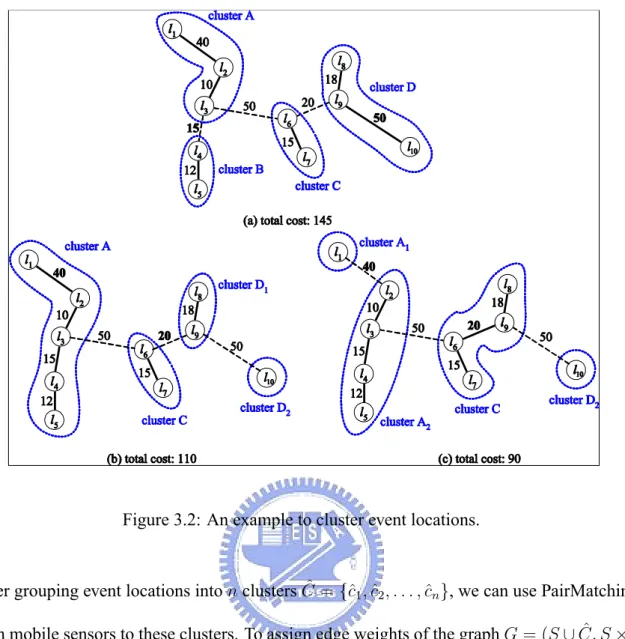
as the total edge weight of the minimum spanning tree in that cluster, where the weight of an edge (li; lj) is the Euclidean distance of the two event locations li and lj. For example, in Fig. 3.2(a),

(A) = 50, (B) = 12, (C) = 15, and (D) = 68. Unfortunately, K-means cannot guarantee to minimize the total cost of the clusters derived, especially when some “sparse” event locations are far away from others. In this case, K-means will group these sparse event locations into the same cluster, thereby increasing the total cost of clusters. Consider an example in Fig. 3.2(a), where four clusters are determined by K-means. Since both clusters A and D consist of sparse event locations (i.e., l1 and l10), the total cost of clusters is thus increased. By properly splitting and merging some

clusters, we could adjust the result of K-mean so as to reduce the total cost of clusters. Intuitively, those clusters containing sparse event locations should be split. However, in order not to change the number of clusters, we have to merge two clusters when splitting a large one. In particular, let max_intra_cost be the maximum edge weight among edges in all clusters and min_inter_cost be the minimum distance of two clusters, where the distance between two clusters ^caand ^cbis the Euclidean

distance of the two closest event locations li and lj, where li 2 ^caand lj 2 ^cb. If max_intra_cost is

larger than min_inter_cost, we can split the cluster with the edge whose weight is max_intra_cost (by removing that edge) and then merge two clusters whose distance is min_inter_cost (by connecting them with the shortest edge). We can repeat the above procedure until max_intra_cost is not larger than min_inter_cost. In this way, we can avoid some clusters having too large costs and thus reduce the total cost of clusters. Fig. 3.2 illustrates an example. In Fig. 3.2(a), max_intra_cost is 50 (in cluster D) and min_inter_cost is 15 (between clusters A and B). We thus split cluster D into two clusters D1 and D2, and then merge clusters A and B into the same one, as shown in Fig. 3.2(b).

Similarly, we can further split cluster A and then merge clusters C and D1to reduce the total cost of

Figure 3.2: An example to cluster event locations.

After grouping event locations into n clusters ^C =_f^c1; ^c2; : : : ; ^cng, we can use PairMatching to

dispatch mobile sensors to these clusters. To assign edge weights of the graph G = (S [ ^C; S C),^ the energy cost function should be re-formulated as follows:

c(si; ^ck) = move (d(si; lj) + (^ck));8si 2 S and ^ck2 ^C;

where lj 2 ^ck is the closest event location to si. Speci cally, the total energy energy consumption

for si to visit ^ck includes the energy to move to the closest event location lj in ^ck and the energy

to reach all event locations in ^ck. Once the graph G is constructed, we can adopt PairMatching to

decide which mobile sensor should be dispatched which cluster. When si is dispatched to a cluster

^

ck, it rst moves to the closest event location lj in ^ck and then exploits the solution of the traveling

Algorithm 2 CentralSD

Input: sets of event locations L and mobile sensors S Output: dispatch schedules fSCHs1; SCHs2; : : : ; SCHsng

1: if jSj jLj then

2: P = PairMatching(L, S); 3: while (si; lj)2 P do

4: SCHsi =fljg;

5: end while

6: else /* event locations are more than mobile sensors */ 7: group locations in L into n clusters by K-means; 8: repeat

9: compute max_intra_cost and min_inter_cost; 10: if max_intra_cost > min_inter_cost then 11: split the cluster with max_intra_cost; 12: merge the two clusters with min_inter_cost; 13: until max_intra_cost min_inter_cost

14: let ^C =_f^c1; ^c2; : : : ; ^cng be the set of clusters;

15: P = PairMatching( ^C, S); 16: while (si; ^ck)2 P do

17: travel all locations in ^ckby TSP and add these

locations into SCHsi in sequence;

3.2 Algorithm GridSD: A Distributed Dispatch Method

In CentralSD, a central server is needed to collect the information of mobile sensors and events, which results in a large amount of message transmissions. To reduce the messages incurred, we propose a distributed algorithm GridSD that explores a grid-based architecture, in which each grid head will collect the information of mobile sensors and events and performs CentralSD locally. Therefore, both the computation complexity and message transmissions can be greatly reduced.

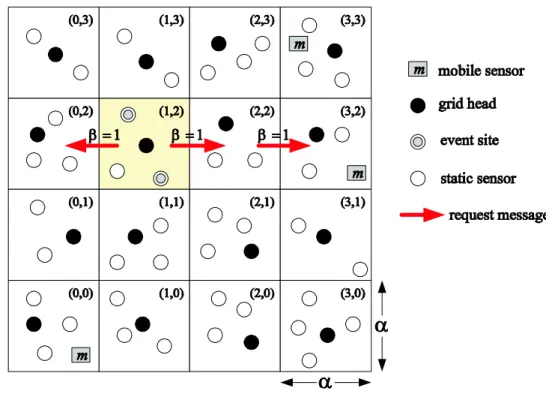
In GridSD, the sensing eld is divided into grids, where each grid is an square, as shown in Fig. 3.3. For each grid, we select a grid head [13] to collect the information such as the numbers of mobile sensors and event locations within its territory. Speci cally, each mobile sensor will inform its location and remaining energy to its corresponding grid head. When detecting events, static sensors will report to their grid head. As pointed out earlier, once obtaining such information, a grid head will perform CentralSD to dispatch mobile sensors to those events occurred in its grid. However, if no mobile sensors available in this grid, the grid head will search available mobile sensors in other grids.

To reduce the number of message transmissions when a grid head searches for mobile sensors in other grids, we propose a modi ed approach of the grid-quorum [20]. Speci cally, each grid head will send advertisement (ADV) messages containing the number of mobile sensors in its grid to the same column of grids. In this way, each grid head will have the information of mobile sensors in other grids located in the same column. When a grid head wants to search for available mobile sensors in other grids, it will send a request (REQ) message to the grid head in the same row. Clearly, due to the grid structure, there must be a grid head that receives both the ADV and REQ messages. Consider Fig. 3.3 as an example, where the grid head in (0; 0) sends an ADV message to inform the grids (0; 1), (0; 2), and (0; 3) that a mobile sensor is available in grid (0; 0). Since there is no available mobile sensor in grid (1; 2), its grid head will send an REQ messages to the grids (0; 2), (2; 2), and (3; 2) to search available mobile sensors. It can be seen that the grid head in (0; 2) will

receive both the ADV and REQ messages and then can reply the available mobile sensors in grid (0; 0)to the grid head of (1; 2).

To further reduce the message transmission for searching available mobile sensors, we exploit search length to limit the number of grids to be searched. Explicitly, each REQ message is asso-ciated with two integers and Mgrid, where is the search length and Mgrid records the number

of available mobile sensors found. Due to the load-balance features, one would like to get as many available mobile sensors as possible. That is why we use to restrict searching length and within the search lengths, all available mobile sensors rather than the nearest one will be considered for dispatching. Initially, > 0and Mgrid = 0in each REQ message. When receiving the REQ

mes-sage, a grid head will increase Mgrid by the number of mobile sensors in this column since the ADV

messages from the grid heads in the same column will publish the available mobile sensors in this column. If > 1, the grid head will decrease by one and then propagate the REQ message to the next grid in the same row. However, if = 1and the value of Mgrid is still zero, which means that

there is no mobile sensor found yet, the grid head will send the REQ message with = 1to the next grid until at least one mobile sensors are available. Fig. 3.3 illustrates an example, where = 1in the initial REQ message. When receiving the REQ message, the grid head in (0; 2) increases Mgrid

by one and decreases by one. Since the value of becomes zero, the REQ message will not be propagated toward the left-hand side. When the grid head in (2; 2) gets the REQ message, it nds that = 1 and Mgrid = 0. So the grid head in (2; 2) propagates the REQ message with = 1 to grid

(3; 2)for searching mobile sensors. By exploring the search length, GridSD can reduce not only the message complexity but also the competition of mobile sensors from grid heads. Once obtaining the information of mobile sensors and events, a grid head is able to perform CentralSD locally.

Algorithm 3 GridSD

AT EACH GRID HEAD WITH EVENT LOCATIONS Notations:

Lgrid is the set of event locations in this grid.

Sgrid is the set of mobile sensors found.

Procedure:

1: send REQ with > 1and Mgrid = 0to the same row;

2: collect the information of Sgrid from neighboring grid;

3: execute CentralSD with Lgrid and Sgrid;

4: send dispatch schedules to the mobile sensors in Sgrid;

AT EACH GRID HEAD WITH MOBILE SENSORS 1: send ADV to the same column;

2: if receive a dispatch schedule then

3: dispatch the mobile sensor according to the schedule; 4: remove the departing mobile sensor;

AT EACH GRID HEAD Notation:

Mcurrent is the number of mobile sensors in the column.

Procedure:

1: If receive an REQ then 2: Mgrid Mgrid + Mcurrent;

3: If = 1and Mgrid = 0then

4: _1; 5: else

6: 1;

7: reply the information to the REQ's originator; 8: If then

Chapter 4

Experimental Results

In this chapter, we evaluate the performances of our proposed algorithms by simulations. We set up a sensing eld as a 450m 300m rectangle, on which there are 400 static sensors and several mobile sensors uniformly and randomly deployed, respectively. Each mobile sensor has an initial energy of 3960J (joule) reserved for movement and the moving energy consumption per meter is set to 8.27J [15]. In this chapter, the energy consumption refers to the one caused by the movements of mobile sensors. The communication distances of static and mobile sensors are set to 150m and 80m, respectively, so that all sensors can form a connected network.

4.1 Effectiveness of CentralSD and GridSD

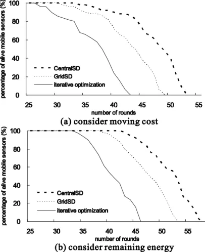
In the rst experiment, we investigate the system lifetime under various dispatching algorithms. We dispatch 50 mobile sensors to visit event locations round by round. During each round, there are 10 to 15 static sensors randomly selected as the event locations. Mobile sensors will then move to these event locations according to the dispatch algorithms and stay at their last-visiting locations to wait for the next dispatch schedule. We mainly observe the percentage of alive mobile sensors during each round. When the number of alive mobile sensors is fewer than that of event locations, the proposed clustering scheme is adopted to group event locations. The system lifetime is referred as

the round when the percentage decreases to zero (i.e., all mobile sensors exhaust their energies). We compare our proposed CentralSD and GridSD against the iteratively-optimized algorithm mentioned in Chapter 1.

Fig. 4.1 shows the system lifetimes when two objective functions Eqs. (2.1) and (2.2) are used (i.e., minimizing the moving cost and maximizing the remaining energy). As can be seen, when the remaining energy of mobile sensors is considered, all the three algorithms will have a longer sys-tem lifetime. The iteratively-optimized algorithm always has the shortest syssys-tem lifetime, although dispatching mobile sensors with the minimal energy cost during each round. This is because the iteratively-optimized algorithm does not balance the loads of mobile sensors, which causes some mobile sensors early to exhaust their energies. The situation becomes worse because these early-exhausted mobile sensors will burden the remaining alive ones with heavy loads. Our proposed algorithms have a longer system lifetime since they not only try to satisfy the objective function but also balance the loads of mobile sensors. Note that CentralSD outperforms GridSD because it has the global knowledge of the network.

4.2 The Impact of Load-Balance

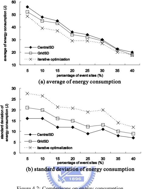
We further evaluate these three dispatch algorithms in terms of the objective function and the load-balance metric (i.e., the standard deviation) among mobile sensors. We use Eq. (2.1) as the objective function and evaluate the average of energy consumption when different dispatch algorithms are adopted. The event locations are randomly selected from 5% to 40% of static sensors. To fairly compare the standard deviation, we set the number of mobile sensors as equal to that of event locations, so that each mobile sensor will be dispatched to exactly one event location.

Fig. 4.2(a) illustrates the average of energy consumption. Since the iteratively-optimized algo-rithm always nds the optimal solution in each round, it will have the smallest average of energy consumption. By adopting the preference lists, the averages of our proposed algorithms will be

Figure 4.2: Comparisons on energy consumption.

slightly higher than that of the optimal solution. Note that in GridSD, the use of search length will prevent the grid heads with event locations from searching those mobile sensors far away from them, thereby having a smaller average compared with CentralSD. Fig. 4.2(b) shows the standard devia-tion of energy consumpdevia-tion. We can observe that the standard deviadevia-tion of the iteratively-optimized algorithm is twice than that of CentralSD, which indicates that the former results in seriously unbal-ance loads among mobile sensors. Note that GridSD has a larger standard deviation compared with CentralSD since each grid head only has partial information of mobile sensors.

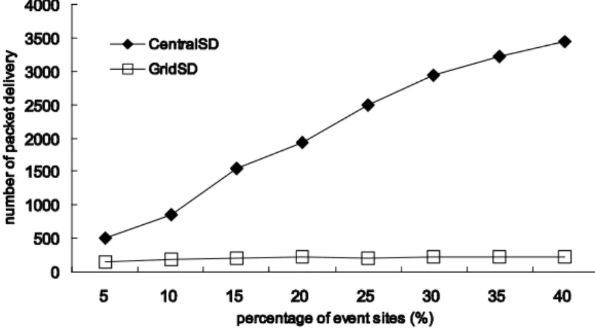
Although CentralSD outperforms GridSD in terms of system lifetime and load-balance, Cen-tralSD incurs a large amount of message transmissions. Fig. 4.3 illustrates the number of packet delivery of CentralSD and GridSD with the number of events varied. We can observe that the

num-Figure 4.3: Comparison on number of packet delivery.

ber of message transmissions in CentralSD grows very fast as the event locations increase, while that in GridSD remains constant because the loads of message exchange are distributed among grid heads.

4.3 The Impact of Clustering

When the number of event locations is larger than that of mobile sensors, we will group event locations into clusters and each mobile sensor will be dispatched to one cluster. Fig. 4.4 shows the effect of clustering scheme on the average of energy consumption. As can be seen, when the clustering scheme is adopted, mobile sensors can have a lower energy consumption because they do not need to travel around event locations far from each other.

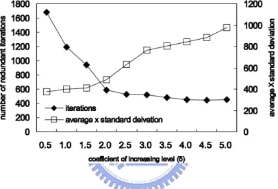
4.4 Sensitivity Analysis on the Coef cient

We nally examine the impact of the coef cient on the increasing level Bin Eq. (3.1). The value

of affects both the computation time and result of PairMatching, as shown in Fig. 4.5. Speci cally, we use the number of redundant iterations that an event location has to repeat Eq. (3.1) to nd an available mobile sensor as the metric to measure the computation time. To evaluate the result of PairMatching, we use the product of average and standard deviation of energy consumption. Clearly,

Figure 4.4: The effect of clustering on energy consumption.

Figure 4.5: The effect of coef cient on redundant iterations and energy consumption, where jLj = jSj = 50.

a smaller product means a better result since mobile sensors can have a lower energy consumption and a more balanced load. Fig. 4.5 shows the effect of coef cient on redundant iterations and energy consumption. We can observe that a smaller will cause more redundant iterations while a larger will make mobile sensors consume more energy and become unbalanced. From Fig. 4.5, we suggest the optimal value of coef cient as 2:0 because both the redundant iterations and the product can be minimized.

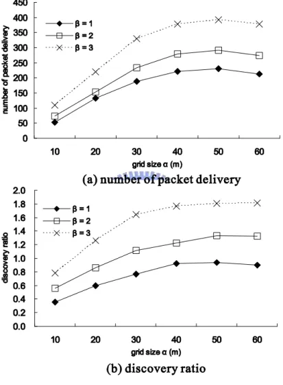
4.5 Effect of grid size

and search length

In Section 3.2, there are two parameters, grid size and search length , used in the GridSD scheme. Fig. 4.6 shows the effects of these two parameters on the number of packet delivery and the discovery ratio. Here we de ne the discovery ratio as 1

N

PN i=1

ni

mi, where N is the number of grids, mi is the

number of event locations in a grid i, and ni is the total number of mobile sensors found by the

head of grid i with the search length . Intuitively, the larger the discovery ratio is, the more mobile sensors a grid head can nd. From Fig. 4.6, we can observe that both the message transmissions and the discovery ratio increase as the grid size and the search length increase. This is because the searching range (to nd available mobile sensors) expands and thus grid heads have to exchange more messages.

Although we can increase the number of mobile sensors found by a grid head by increasing both the values of and , grid heads have to exchange more messages. To obtain a reasonable discovery ratio while not to increase too many message transmissions, we suggest to use = 30and = 2 in this experiment since it has a discovery ratio slightly higher than one. In this case, the number of found mobile sensors will approximate to the number of event locations in a grid.

Figure 4.6: The effects of grid size and search length on the number of packet delivery and the discover ratio, where jLj = jSj = 50.

Chapter 5

Conclusions

In this paper, we have considered how to ef ciently dispatch mobile sensors in a hybrid sensor net-work. By exploring the load-balance of mobile sensors, we have proposed an algorithm CentralSD to dispatch mobile sensors. When the locations are more than the mobile sensors, we developed a clustering scheme to group event locations so that our proposed algorithm is able to apply. In order to reduce the message transmissions, we have also proposed a distributed algorithm GridSD. Simu-lation results showed that our proposed algorithms can have a longer system lifetime compared with the iteratively-optimized algorithm.

Bibliography

[1] I. F. Akyildiz, W. Su, Y. Sankarasubramaniam, and E. Cayirci, “A survey on sensor networks,” IEEE Commun. Mag., vol. 40, no. 8, pp. 102–114, 2002.

[2] P. Basu and J. Redi, “Movement control algorithms for realization of fault-tolerant ad hoc robot networks,” IEEE Network, vol. 18, no. 4, pp. 36–44, 2004.

[3] M. Bläser, “A new approximation algorithm for the asymmetric TSP with triangle inequality,” in ACM-SIAM Symp. on Discrete Algorithms, 2003, pp. 638–645.

[4] N. Bulusu, J. Heidemann, and D. Estrin, “GPS-less low-cost outdoor localization for very small devices,” IEEE Personal Commun. Mag., vol. 7, no. 5, pp. 28–34, 2000.

[5] Z. Butler and D. Rus, “Event-based motion control for mobile-sensor networks,” IEEE Perva-sive Computing, vol. 2, no. 4, pp. 34–42, 2003.

[6] T. A. Dahlberg, A. Nasipuri, and C. Taylor, “Explorebots: a mobile network experimenta-tion testbed,” in ACM SIGCOMM Workshop on Experimental Approaches to Wireless Network Design and Analysis, 2005, pp. 76–81.

[7] J. Han and M. Kamber, Data Mining: Concepts and Techniques, D. D. Cerra, Ed. Academic Press, 2001.

[8] N. Heo and P. K. Varshney, “Energy-ef cient deployment of intelligent mobile sensor net-works,” IEEE Trans. on Syst., Man and Cybern. A, vol. 35, no. 1, pp. 78–92, 2005.

[9] B. Hofmann-Wellenhof, H. Lichtenegger, and J. Collins, Global Positioning System: Theory and Practice. 4th ed., Springer Verlag, 1997.

[10] L. Hu and D. Evans, “Localization for mobile sensor networks,” in Int'l Conf. on Mobile Com-puting and Networking, 2004, pp. 45–57.

[11] D. Johnson, T. Stack, R. Fish, D. M. Flickinger, L. Stoller, R. Ricci, and J. Lepreau, “Mobile Emulab: a robotic wireless and sensor network testbed,” in IEEE INFOCOM, 2006.

[12] H. W. Kuhn, “The Hungarian method for the assignment problem,” Naval Research Logistics Quarterly, vol. 2, pp. 83–97, 1955.

[13] H. Luo, F. Ye, J. Cheng, S. Lu, and L. Zhang, “TTDD: Two-tier data dissemination in large-scale wireless sensor networks,” Wireless Networks, vol. 11, pp. 161–175, 2005.

[14] M. D. Naish, E. A. Croft, and B. Benhabib, “Dynamic dispatching of coordinated sensors,” in IEEE Int'l Conf. on Systems, Man, and Cybernetics, 2000, pp. 3318–3323.

[15] M. Rahimi, H. Shah, G. S. Sukhatme, J. Heideman, and D. Estrin, “Studying the feasibility of energy harvesting in a mobile sensor network,” in IEEE Int'l Conf. on Robotics and Automa-tion, 2003, pp. 19–24.

[16] Y. C. Tseng, Y. C. Wang, and K. Y. Cheng, “An integrated mobile surveillance and wireless sensor (iMouse) system and its detection delay analysis,” in ACM Int'l Symp. on Modeling, Analysis and Simulation of Wireless and Mobile Systems, 2005, pp. 178–181.

[17] A. Verma, H. Sawant, and J. Tan, “Selection and navigation of mobile sensor nodes using a sensor network,” in IEEE Int'l Conf. on Pervasive Computing and Communications, 2005, pp. 41–50.

[18] G. Wang, G. Cao, and T. L. Porta, “A bidding protocol for deploying mobile sensors,” in IEEE Int'l Conf. on Network Protocols, 2003, pp. 315–324.

[19] G. Wang, G. Cao, and T. L. Porta, “Movement-assisted sensor deployment,” in IEEE INFO-COM, 2004, pp. 2469–2479.

[20] G. Wang, G. Cao, T. L. Porta, and W. Zhang, “Sensor relocation in mobile sensor networks,” in IEEE INFOCOM, 2005, pp. 2302–2312.

[21] Y. Zou and K. Chakrabarty, “Sensor deployment and target localization based on virtual forces,” in IEEE INFOCOM, 2003, pp. 1293–1303.