應用分類元系統於財務危機預警之研究

全文

(1)國立交通大學資訊管理研究所碩士論文. 應用分類元系統於財務危機預警之研究 Applying Classifier Systems in Financial Distress Prediction Modeling. 研究生：蔡毓耕指導教授：陳安斌博士. 中華民國九十三年六月.

(2) 應用分類元系統於財務危機預警之研究 Applying Classifier Systems in Financial Distress Prediction Modeling 研究生：蔡毓耕指導教授：陳安斌. Student：Yu-keng Tsai Advisor：An-Pin Chen. 國立交通大學資訊管理研究所碩士論文. A Thesis Submitted to Institute of Information Management College of Management National Chiao Tung University in partial Fulfillment of the Requirements for the Degree of Master in Information Management June 2004 Hsinchu, Taiwan, Republic of China. 中華民國九十三年六月.

(3) 應用分類元系統於財務危機預警之研究學生：蔡毓耕. 指導教授：陳安斌. 國立交通大學資訊管理研究所碩士班. 中文摘要. 財務危機預警對於公司的內部或外部利害關係人，一直是個重要的議題。早期學者多運用區別分析、logistic 迴歸模型、或是 probit 迴歸模型等統計方法建立財務危機預警模型。然而，近年來許多已研究證實，諸如類神經網路(NNs)之人工智慧方法學對於分類問題(ex.預測公司財務危機)有較優異的表現。即使有些學者運用 NNs 預測財務危機得到有效的結果，但由於對資料之敏感性的關係，因而不易建構適當的架構；且在使用模型時，無法提供清楚解釋結果的能力，造成使用之不易。本研究的主要目的為應用 XCS 分類元系統來建置公司財務危機預警模型。由於 XCSR 模型(一種 XCS 分類元系統的延伸模型)結合了增強式學習(Reinforcement learning) 與演化式計算(Evolutionary computation)，因此具備優良的預測能力。且模型中的規則對於預測的結果具可讀性，公司的利害關係人因而較容易了解預測的結果。經由本研究的實證，結果顯示 XCSR 模型的預測能力將顯著優於比較的 logistic 迴歸模型，以精確度而言，XCSR 模型高達 86.8%，logistic 迴歸模型只有 79.9%。另外，文中亦針對 XCSR 所得之規則，與 logistic 迴歸模型做一討論與比較。關鍵字：財務危機，財務比率，分類元系統，XCS 分類元系統。. i.

(4) Applying Classifier Systems in Financial Distress Prediction Modeling Student：Yu-Keng, Tsai. Advisor：An-Pin Chen. Institute of Information Management National Chiao Tung University. ABSTRACT. The prediction of financial distress is an important and active topic since it is critical to all stakeholders both internal and external to the company. Earlier studies of financial distress prediction used statistical approaches such as multiple discriminant analysis, logistic regression and probit model. Recently, however, several studies have demonstrated that artificial intelligence methodology such as neural networks (NNs), has the superior abilities on classification problems. Even though some of the studies using NNs to the prediction of financial distress have reported its usefulness, there are still several drawbacks in developing and using these models. The sensitivity of financial data would affect building an appropriate model and the learning results could not be read comprehensibly.. The purpose of this paper is to propose XCS classifier systems approach and illustrate how the XCSR model (one model extended from XCS classifier systems) can be applied to financial distress. The exploitation of reinforcement learning and evolutionary computation constitutes a considerably advantage for the XCSR model to provide the superiorly predictive. ii.

(5) ability. Also, the obtained regularities are a means of easily understanding for the stakeholders of a firm.. The results obtained with the XCSR model showed to be significantly superior to those obtained from the benchmark model (the logistic regression model). The XCSR model has a better accuracy, it is 86.8% accuracy compared to logistic regression model, which only has 79.9% accuracy. Moreover, the extracted regularities were discussed for the increased understanding when comparing to the logistic regression model.. Key words: Financial Distress, Financial Ratio, Classifier Systems, XCS Classifier Systems.. iii.

(6) ACKNOWLEDGEMENTS. My sincere thanks are due to Professor An-Pin Chen. Both the researching and living supports throughout my graduate studies have assisted me greatly. Also, acknowledgements and thanks are given to the other members of my committee: Ching-Hsue Cheng, Ja-Shan Chen, and Duen-Ren Liu, for their helpful comments and suggestions. On the other hand, I want to thank my friends who have helped and encouraged me during the process of finishing my thesis, especially Wen-Chich Tsai for his coaching.. Finally, a special thank to my girl friend, Chia-Chi Lin, for her patience and encouragement during this whole research process. Thanks also to my family without whom I would never be a master. I would like them to understand how much they have made me proud.. iv.

(7) Contents 中文摘要 .....................................................................................................................................i ABSTRACT ...............................................................................................................................ii ACKNOWLEDGEMENTS ......................................................................................................iv Contents ......................................................................................................................................v List of Tables ............................................................................................................................vii List of Figures..........................................................................................................................viii Chapter 1: Introduction...............................................................................................................1 1.1 Motivation.....................................................................................................................1 1.2 Purpose.........................................................................................................................3 1.3 Thesis Organization......................................................................................................4 Chapter 2: Literature Review......................................................................................................6 2.1 Definition of Financial Distress ...................................................................................6 2.2 Overview of Financial Distress Prediction Models....................................................10 2.3 Overview of the explanatory variables.......................................................................14 2.4 Overview of Classifier Systems ..................................................................................16 Chapter 3: XCS Classifier Systems ........................................................................................19 3.1 Overview of XCS.........................................................................................................19 3.2 Terminology and Notation ..........................................................................................20 3.2.1 A classifier in XCS...........................................................................................20 3.2.2 The different sets..............................................................................................23 3.3 The framework of XCSR .............................................................................................23 3.3.1 Performance component..................................................................................24 3.3.2 Reinforcement component ...............................................................................25 3.3.3 Discovery component ......................................................................................27 3.4 Summary .....................................................................................................................30 Chapter 4: Research Design .....................................................................................................31 4.1 Research Architecture.................................................................................................32 4.2 Sample Selection.........................................................................................................33 4.2.1 Selection Criteria.............................................................................................33 4.2.2 Experimental Data...........................................................................................34 1. Research Scope.............................................................................................34 2. Data Sources.................................................................................................35 4.2.3 Research variables...........................................................................................35 4.3 Research limitation.............................................................................................42 4.4 Implementation Models ..............................................................................................43 v.

(8) 4.4.1 XCSR Model ....................................................................................................43 4.4.2 Logistic Regression Model ..............................................................................44 4.5 Statistical Test Description .........................................................................................45 1. Description of Test for Classification Accuracy ...........................................45 2. Description of Test for Differences between Two Models’ Accuracy............46 3. Description of Test for Tendency ..................................................................47 Chapter 5: Results and Discussions..........................................................................................48 5.1 Logistic Regression Model .........................................................................................48 1. Collinearity Tests ..........................................................................................48 2. Level of fit .....................................................................................................49 3. Classification Results ...................................................................................51 5.2 XCSR Model ...............................................................................................................53 5.3 Differences of predictive accuracy between two models ............................................55 5.4 Tendency of accurate rates for the distressed companies...........................................56 5.5 Regularities.................................................................................................................57 Chapter 6: Conclusions.............................................................................................................60 6.1 Conclusions ................................................................................................................60 6.2 Future Works...............................................................................................................61 Reference ..................................................................................................................................62. vi.

(9) List of Tables Table 2.1 Summary of definition of financial distress................................................................8 Table 2.2 The frameworks of accounting ratios .......................................................................15 Table 2.3 Ratio framework announced by SFC........................................................................16 Table 3.1 Three classifier examples..........................................................................................21 Table 3.2 Three examples of classifiers taking real values ......................................................22 Table 4.1 Sample distribution by year ......................................................................................35 Table 4.2 Selected variables [47]..............................................................................................38 Table 5.1 Collinearity tests for each variable ...........................................................................49 Table 5.2 Level of fit ................................................................................................................50 Table 5.3 Classification results of the logistic regression model .............................................51 Table 5.4 Type I and Type II error description .........................................................................52 Table 5.5 Classification results of the XCSR model ................................................................54 Table 5.6 test of differences between two models....................................................................55 Table 5.7 Tendency Test Result ................................................................................................56 Table 5.8 Examples of regularities ...........................................................................................57 Table 5.9 Profile analyses.........................................................................................................58. vii.

(10) List of Figures Figure 1.1 Thesis organization ...................................................................................................5 Figure 3.1 The learning structure of XCS [36].........................................................................19 Figure 3.1 The framework of XCS [3]. ....................................................................................24 Figure 3.2 Flowchart of GA in XCS.........................................................................................28 Figure 4.1 Research Architecture .............................................................................................32 Figure 4.2 the time point of announcing financial statement [46] ...........................................36 Figure 4.3 Time point selection ................................................................................................37. viii.

(11) Chapter 1: Introduction. 1.1 Motivation. The likelihood of financial distress has been an active issue for a long time. It is against the “going concern” assumption and it is critical to many stakeholders both internal and external to the firm. In Taiwan, a series of financial distressed events had started from the second half of 1998, therefore, further shows the importance of this topic.. Many researches have been devoted to the development of financial distress prediction models for providing the solutions to this topic. Earlier studies of financial distress prediction utilized statistical approaches such as multiple discriminant analysis (MDA) (Altman [1], [2]), logit model (Ohlson [3], Shih [4]), and probit model (Zmijewski [5]). However, the restrictive statistical assumption of these conventional statistical methods, such as the required linearity, normality and independence among input variables, is the main problem of implementing them. Recently, several studies have demonstrated that artificial intelligence methodology such as neural networks (NNs), has the superior abilities on classification problems [6]. Even though, since 1990, some of the studies using NNs to the prediction of financial distress have reported its usefulness, there are several drawbacks in developing and using them. The sensitivity of financial data would affect building an appropriate structure [7, 8], and the learning results could not be read comprehensibly [6, 9].. A learning machine paradigm in artificial intelligence, called the “classifier systems”, is a combination of evolutionary computation and reinforcement learning. A set of condition-action rules (i.e., the classifiers) is developed in classifier systems, which is suitable. 1.

(12) for prediction and classification. Also rules are a useful means to represent knowledge for the applied problems. Classifier systems have been actively developed during the recent years. Many models have been proposed during this developing period. Some of the important features of the systems like its adaptivity and generalization make it successfully when applying to many domains. Therefore, the purpose of this paper is to exploit classifier systems (XCS classifier systems actually, the most promising and applied) and to develop a financial distressed prediction model. Also, to work towards the goal of providing stakeholders of the firm with a more accurate prediction model that consists of rules representing the information about the predicted company.. 2.

(13) 1.2 Purpose. The purpose of this paper is to provide a method that can identify the likelihood of financial distress for the company stakeholders. It can be accomplished by taking quantitative data (financial ratios), processing it into a form that can be used by the XCSR model (one model extended from XCS classifier systems), and predicts financial distress or non-distress. That is, the XCSR model was developed through the use of financial ratios in order to achieve this purpose.. The predicted results of the XCSR model were then compared to a benchmark. A logistic regression model was developed as the benchmark using the same data source. In addition to the comparison of predictive power, the rules obtained from the XCSR model were discussed to the objective of extensive understanding of the financial phenomena to every company. Consequently, to accomplish the purpose, comparisons to the benchmark model and the discussions to the rules provided by the XCSR model were done.. 3.

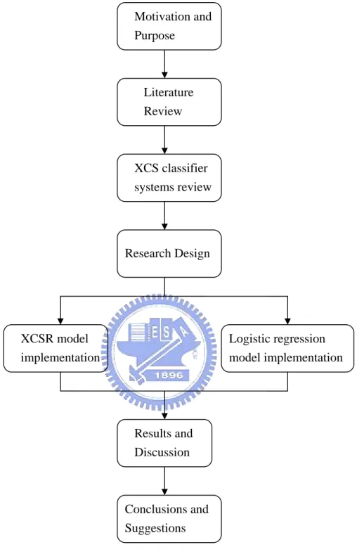
(14) 1.3 Thesis Organization This paper was divided into six chapters, and the following gives the detail descriptions of each chapter. Chapter 1 Introduction --The purpose and motive of conducting this research were described in this chapter. Chapter 2 Literature Review --Reviewed on past researches on financial distress prediction: the definitions of financial distress, the history of financial distress prediction studies, the frameworks of explanatory variables, and an introduction to classifier systems. Chapter 3 XCS Classifier Systems --Following section 2.4, this chapter gave more detail descriptions about XCS Classifier Systems, which include the descriptions of terminology and framework. Chapter 4 Research Design --This chapter gave details about research architecture. The descriptions about the flows of architecture were given. Chapter 5 Results and Discussions --This chapter presented the summarized results of the XCS model and the logistic regression model. The comparisons about the two models and the rules obtained from the XCS model were discussed. Chapter 6 Conclusions --The conclusion of result between the two models, and the suggestion of doing further studies were given here.. Figure 1.1 shows the organization of this paper.. 4.

(15) Motivation and Purpose. Literature Review. XCS classifier systems review. Research Design. XCSR model implementation. Logistic regression model implementation. Results and Discussion. Conclusions and Suggestions. Figure 1.1 Thesis organization. 5.

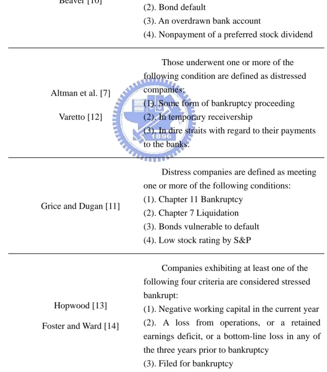
(16) Chapter 2: Literature Review. 2.1 Definition of Financial Distress. A large amount of models have been developed to predict corporate health. Unfortunately, little agreement exists regarding to definite definition of “Financial Distress”. Table 2.1 summarized some of the definitions in priori studies.. Table 2.1 shows that Taiwan differs from the world others on the definition of distressed company. Numerously foreign studies, called bankruptcy prediction, concentrated on those filed for bankruptcy [1, 3, 5, 6, 8]. These companies usually declared relevant bankruptcy legislation in their country (mainly in America). Some other researchers extended their definition to a more general one. The models can distinguish the difference between a healthy firm and an unsound one. But unlike the previous model, this one can also distinguish the different between a healthy firm, and a bankruptcy firm [7, 10, 11, 12, 13, 14]. In other words, the definitions of financial distress are due to the legislation and some perceptions extended by researchers. Therefore, the differences of national condition from other countries result in the distinct definitions of financial distress. Domestically, the legislations concerning financial distress are: article 49、article 50、and article 50-2 of “Operating Rules of the Taiwan Stock Exchange Corporation”, plus article 211 and article 282 of “Company Law”. The representative events are “listed securities placed under altered-trading-method category, trading been suspended, listing been terminated, declaring bankruptcy, or declaring reorganization”. The number of company declaring bankruptcy in Taiwan [15] was quite few when comparing to other foreign cases. Therefore, they were adopted all together as the definition of financial distress in early studies [16, 17, 18, 6.

(17) 19]. However, the latter studies indicated that the financial difficulties should happen in earlier stage [15, 20, 21]. Companies could encounter more or less financial troubles prior to the above-mentioned events. Therefore, recent studies extended relevant events (as in table 2.1) to their operating definitions of financial distress.. To sum up, the differences of national condition among different countries resulted in the distinct definitions of financial distress. Consequently, consider the case in Taiwan, the related legislation and previous studies would be referred as the main definitions of financial distress in this paper.. 7.

(18) Table 2.1 Summary of definition of financial distress Researcher. The definition of financial distress. Altman [1], Ohlson [3], Zmijewski [5] , Shin and Lee [6], Boritz and Kennedy [8]. Beaver [10]. Altman et al. [7] Varetto [12]. Grice and Dugan [11]. Hopwood [13] Foster and Ward [14]. Companies filed for bankruptcy.. Failed companies are defined as meeting one or more of the following conditions: (1). Bankruptcy (2). Bond default (3). An overdrawn bank account (4). Nonpayment of a preferred stock dividend Those underwent one or more of the following condition are defined as distressed companies: (1). Some form of bankruptcy proceeding (2). In temporary receivership (3). In dire straits with regard to their payments to the banks. Distress companies are defined as meeting one or more of the following conditions: (1). Chapter 11 Bankruptcy (2). Chapter 7 Liquidation (3). Bonds vulnerable to default (4). Low stock rating by S&P Companies exhibiting at least one of the following four criteria are considered stressed bankrupt: (1). Negative working capital in the current year (2). A loss from operations, or a retained earnings deficit, or a bottom-line loss in any of the three years prior to bankruptcy (3). Filed for bankruptcy. 8.

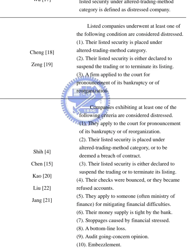
(19) Table 2.1 Continued Researcher. Hwang [16] Wu [17]. Cheng [18] Zeng [19]. Shih [4] Chen [15] Kao [20] Liu [22] Jang [21]. The definition of financial distress According to article 49 of “Operating Rules of the Taiwan Stock Exchange Corporation”, listed company which place their listed security under altered-trading-method category is defined as distressed company. Listed companies underwent at least one of the following condition are considered distressed. (1). Their listed security is placed under altered-trading-method category. (2). Their listed security is either declared to suspend the trading or to terminate its listing. (3). A firm applied to the court for pronouncement of its bankruptcy or of reorganization. Companies exhibiting at least one of the following criteria are considered distressed. (1). They apply to the court for pronouncement of its bankruptcy or of reorganization. (2). Their listed security is placed under altered-trading-method category, or to be deemed a breach of contract. (3). Their listed security is either declared to suspend the trading or to terminate its listing. (4). Their checks were bounced, or they became refused accounts. (5). They apply to someone (often ministry of finance) for mitigating financial difficulties. (6). Their money supply is tight by the bank. (7). Stoppages caused by financial stressed. (8). A bottom-line loss. (9). Audit going-concern opinion. (10). Embezzlement.. 9.

(20) 2.2 Overview of Financial Distress Prediction Models. Since Beaver [10], one of the first researchers to study the prediction of bankruptcy, prediction of corporate failure is a popular topic so far. Many models were structured by different ratios, sample, and methodologies. Some well-known studies will be reviewed next.. Beaver [10] employed a univariate model to examine the predictability of 6 kinds of financial ratios for business failure. He selected a total of 158 samples including 79 failed firms and 79 non-failed firms from 1954 to 1964. Beaver determined that the cash flow to total debt was the best performing ratio. Net income on total assets, the total debt to total assets were the next two best performing ratios.. Beaver’s research method in his study deserves some credits. His methods included matched-sample design, addition of new financial ratios, and evaluation accuracy through testing samples, etc. Many researchers later on, had been following his methods. However, the univariate analyses are questionable both theoretically and practically [1]. They ignore the correlation among the financial ratios of several firms resulting in the potential ambiguity inherent in any univariate analysis. Consequently, it is appropriate to further combine several ratios to build a more appropriate predictive model [1, 10].. After Beaver, the first study that used multiple discriminant analysis (MDA) to discriminate the companies into known categories was done by Altman [1]. He improved Beaver’s paired sample design upon industry type and firm size to select 33 pairs of manufacturing companies in 1946-1965. A combination of five (selected by a stepwise MDA from an original list of 22) financial ratios were used to build a bankruptcy likelihood score, i.e., Altman’s Z-score, as the prediction model. In the short run, it classified quite accurately. 10.

(21) with a predictive power of 95% one year prior to bankruptcy. However, in the long run, the prediction will not be as accurate as in the short run.. After Altman [1], researchers started to apply discriminant analysis extensively to build predicting models [2, 23, 24]. However, the restrictive statistical assumption of the discriminant analysis, which requires multivariate normality and the equality of covariance matrices, is its main problem [25]. Though violating these assumptions is unimportant if the purpose of the model is to be a discriminating device, nevertheless it results in selection of an inappropriate set of measures [3, 25].. Ohlson [3] addressed this problem and introduced the logistic regression techniques to estimate the probability of bankrupt/non-bankrupt for a company. He utilized nine ratios for his analysis, based on simplicity, and randomly selected 105 bankruptcy and 2058 healthy firms in 1970 – 1976. Though the results were not obviously better than previous ones, he concluded that his methodology was more robust with avoidance of all the problems discussed with respect to MDA [3].. Because the nature of logistic regression analysis required less statistical requirements, many studies followed Ohlson to apply it [4, 13, 14, 16, 19]. Lo [26] compared these two widely used techniques, logit analysis and MDA, through 38 pairs companies in 1975 – 1983. He suggested that logit is a much more robust technique whatever data distributed. However, MDA will be asymptotically efficient while the restrictive assumptions are satisfied. In other words, Lo [26] indicated that the first choice of prediction model would be the logit approach unless the restrictive assumptions are satisfied. On the other hands, Grice and Dugan [11] indicated the cautions for using logit and probit analysis. They evaluated Ohlson [3] and Zmijewski [5] models that utilized logit and probit analysis, respectively. The empirical findings demonstrated that both models were sensitive to time periods. That is, the accuracy 11.

(22) of the models in the time periods used to develop them was not consistent with that in the different ones. As a result, they suggested that it is necessary to carefully use the models to avoid erroneous applications of bankruptcy prediction models. That is, it should pay attention to the applied period of the models developed by these two methods. Since the sensitivity to data period would result in incorrect applications.. For many years, artificial intelligence approaches which are less restrictive assumptions, such as inductive learning, Neural Networks (NNs), Genetic Algorithms (GAs), and case-based reasoning (CBR), have been shown that they can be alternative methodologies for classification problems to which conventional statistical methods have been long applied [6]. NNs were the mostly applied techniques for the financial distressed prediction since 1990. The following is a review focused on this approach.. The first study to use NNs for the bankruptcy prediction problem was done by Odom and Sharda [27]. Odam and Sharda built the model with five input variables the same as Altman’s financial ratios [1]. They selected a total of 129 research samples including 65 bankruptcy firms and 64 non-bankruptcy firms between 1975 and 1982, where the ratio data were from the financial statement one year prior to bankruptcy. Among these samples, a training set and testing set, consisting of 74 firms (38 bankrupt and 36 non-bankrupt) and 55 firms (27 bankrupt and 28 non-bankrupt), were selected. An MDA was used on the same training set as a comparison. The results indicated the NNs achieved classification accuracy 81.81% of the hold out sample while the MDA only did 74.28%. Tam and Kiang [28] utilized commercial bank failure data to compare the NNs with several methods: ID3 (a decision tree classification algorithm), MDA, logit, and KNN (K-nearest neighbor). The collected bank data included 59 failed and 59 non-failed banks for the period from 1985 to 1987. Among these models, ID3 and KNN were almost worse than the other methods, and NNs presented more accurate and solid results. 12.

(23) Some domestic studies also used NNs for financial distress prediction, which suggested that the NNs model performed more accurate than the other traditional statistic methods [29, 30]. These studies (mentioned above) all showed the usefulness of using NNs to predict financial distress. However, some studies addressed a number of cautions for applying NNs to financial distress prediction. They are discussed below.. Altman et al. [7] applied NNs and MDA to a large database, consisting of over 1000 healthy, vulnerable, and unsound Italian firms from 1982 – 1992, for one-year-ahead prediction. They concluded that NNs were able to accurately predict companies, even in some cases better than MDA. However, the problems with NNs included: illogical behavior patterns in their NNs systems, overfitting in the training stage, and the resulting weights in NNs structure were sensitive to structural changes. All of them negatively impacts predictive accuracy. The overall comparison resulted in no determinative winner, though MDA was slightly better. Bortiz and Kennedy [8] used the NNs models including different training procedures to compare with Altman’s model (MDA) and Ohlson’s model (Logit). They utilized 6324 (171 bankrupt and 6153 non-bankrupt) companies in 1971 – 1984 with the same ratios chosen by Altman and those chosen by Ohlson. The results showed that the performance of NNs was sensitive to the choice of input variables and that the networks cannot focus on the most important variables through sifting them. Their cautions also indicated the sensitivity of the models to variations in the data. Atiya [9] surveyed numerous financial distress prediction studies on using NNs and presented a NNs model with some novel indicators to improve the accuracy. However, he indicated that one of the existing challenges for the NNs approach is the understanding of the likelihood of financial distress. Statistical methods can show the default probability to assist in recognizing potential distress or non-distress. This is inadequate for the NNs model to show the relevant information.. 13.

(24) The above three studies indicated two parts of drawbacks about developing financial distress model using NNs. First, it is difficult to build an appropriate NNs structure. The sensitivity to input variables and structural changes would be the problems. Second, it could not be readily understood by the users when comparing to statistical approaches. The default probability provided by the statistical methods could assist in comprehending the results, but inadequate for NNs. This feature of NNs is therefore referred to as “black-boxes”. Consequently, these two problems should be the cautions while developing financial distress prediction model through NNs.. To summarize the previous studies, the financial distress prediction models have been developed through statistical and artificial intelligence (mainly NNs) methods. Though statistical methodology has applied to develop the prediction model for a long time, its disadvantage is that it required some restrictive statistical assumptions. The NNs models have been demonstrated to predict more accurate than traditional statistical methods, but the drawbacks of developing and using the model are its limitations.. 2.3 Overview of the explanatory variables. Generally speaking, previous studies utilized one or more financial indicators to the research of predicting financial distress. Mossman et al. [31] mentioned four classes of explanatory variable: financial ratio、cash flow、market-adjusted returns、and standard deviation. They were often used to develop financial distress prediction model. The empirical results indicated that the ratio model presented the most effective in discriminating companies in the year prior to bankruptcy, while the cash flow model offered the most consistent ability to discriminate between bankrupt and non-bankrupt companies in the three years before bankruptcy. In other words, the accounting ratios (financial ratios and cash flow) perform 14.

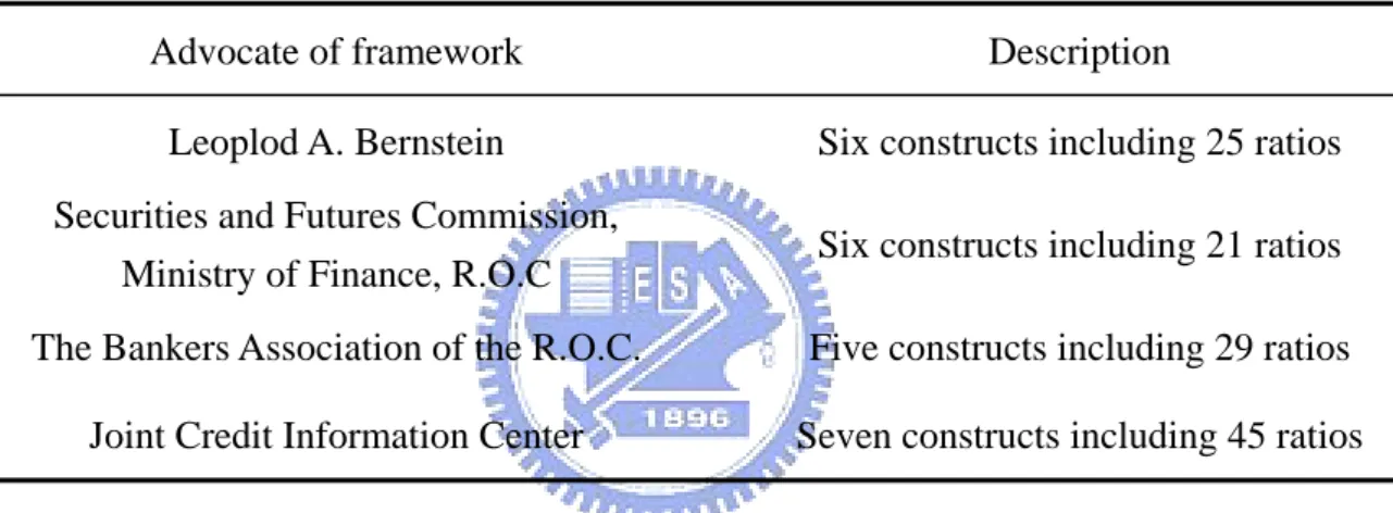
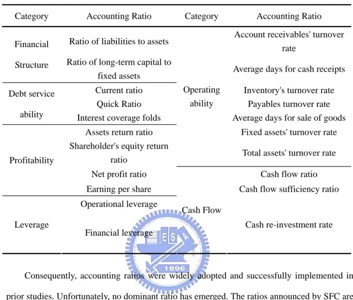
(25) better among these four classes of explanatory variable. Besides, many domestic researchers also used accounting ratios as their indicators to develop models [16, 17, 18, 19]. Therefore, this paper also utilized accounting ratios to develop the financial distress prediction model.. However, although accounting ratios have been successfully implemented to develop models, there exists little agreement regarding to the best accounting ratios to the prediction of financial distress. Table 2.2 summarized some important frameworks of accounting ratios mentioned in Lin [32], which including most of previous studies.. Table 2.2 The frameworks of accounting ratios Advocate of framework. Description. Leoplod A. Bernstein. Six constructs including 25 ratios. Securities and Futures Commission, Ministry of Finance, R.O.C. Six constructs including 21 ratios. The Bankers Association of the R.O.C.. Five constructs including 29 ratios. Joint Credit Information Center. Seven constructs including 45 ratios. From table 2.2, the framework advocated by Securities and Futures Commission, Ministry of Finance, R.O.C (SFC) is important in domestic studies. According to the laws of “Criteria Governing Information to be Published in Public Offering and Issuance Prospectuses” and “Criteria Governing Information to be Published in Annual Reports of Public Companies”, those ratios in the framework should be included in prospectus and annual report. Domestically, the prospectuses and annual reports of companies are the major sources of these ratios. Therefore, the framework announced by SFC is a convinced structure of explanatory variable. Table 2.3 listed those ratios announced by SFC.. 15.

(26) Table 2.3 Ratio framework announced by SFC Category. Accounting Ratio. Financial. Ratio of liabilities to assets. Account receivables' turnover rate. Structure. Ratio of long-term capital to fixed assets. Average days for cash receipts. Debt service ability. Current ratio Quick Ratio Interest coverage folds. Fixed assets' turnover rate. Profitability. Assets return ratio Shareholder's equity return ratio Net profit ratio. Cash flow ratio. Earning per share. Cash flow sufficiency ratio. Operational leverage Leverage. Category. Operating ability. Accounting Ratio. Inventory's turnover rate Payables turnover rate Average days for sale of goods. Total assets' turnover rate. Cash Flow Cash re-investment rate. Financial leverage. Consequently, accounting ratios were widely adopted and successfully implemented in prior studies. Unfortunately, no dominant ratio has emerged. The ratios announced by SFC are an important framework with the essentials of prior studies. Therefore, this framework is the basic structure of explanatory variable in this paper.. 2.4 Overview of Classifier Systems. Classifier systems are intended as a machine learning paradigm first introduced by John H. Holland in 1975. They combine evolutionary computation and reinforcement learning to develop a set of condition-action rules which show the target regularities from unknown environment that the system has learned from on-line experience [33].. 16.

(27) In the early 90s, it appeared that this field was too complex to be studied. Few successful applications had been published. Recently, however, new models have been developed and applied to new domains which resuscitated this area a lot.. Two important characteristics of classifier systems, its adaptivity, and generalization, are important in many application domains such as Computational Economics, Knowledge Discovery, and Data Mining [33]. The adaptivity of classifier systems enables classifier systems to be capable of on-line learning in rapidly changing situations. Generalization is an intriguing and principal feature among them since it makes the system apply what it has learned to previously unobserved situations.. Many applications of classifier systems have been presented [34]. There are three main applied areas consisting of these domains: autonomous robotics, knowledge discovery, and computational economics. In addition to these three areas, there are still other interesting applications. It refers to [34] for more details.. In the past, classifier systems, also called learning classifier systems (LCS), just represented Holland’s LCS and most studies focused on the problems that the original model had. Recently, many different models have been proposed with Holland’s structure as the main building component. LCS is then identified as the paradigm introduced by Holland. Among these models, Wilson’s XCS, Stolzmann’s ACS, and Holmes’ EpiCS appear particularly promising in the recent years [33]. Since XCS is the most studied and applied in recent years, this paper would then focus on it.. Started in 1987, Wilson modified Holland’s ideas to develop a new but simpler LCS. In these years, Wilson’s research experienced some important models (NEWBOOLE, ZCS [35]) which eventually evolved to XCS. Though XCS retains the whole main structure of Holland’s model, it introduces some essential modifications to the previous architecture, which results in 17.

(28) the most promising and the most important breakthrough in LCS research [33]. Regarding to much more description about XCS, it is given in chapter three.. 18.

(29) Chapter 3: XCS Classifier Systems. 3.1 Overview of XCS. XCS classifier systems are a learning machine basically, with a mechanism of reinforcement learning. Figure 3.1 shows the learning structure of XCS.. Environment. Payoffs Inputs Actions. XCS. Figure 3.1 The learning structure of XCS [36]. The system learns to get the maximum of reinforcement, the payoffs returned from the environment in figure 3.1. This is the structure of reinforcement learning to act that the adaptability of XCS is improved with time, by means of interaction with the environment.. The learning process is continuing all the time, as XCS goes along. The goal of this on-line learning is to capture regularities (i.e., rules) from the environment. It represents that those situations that map to equivalent consequences are identified and classified together to be represented by internal structure. It takes the advantages of avoiding an extra demand on storage of the raw environmental data. It is an ability to be toward generalization, which is a natural tendency of XCS [33, 37].. 19.

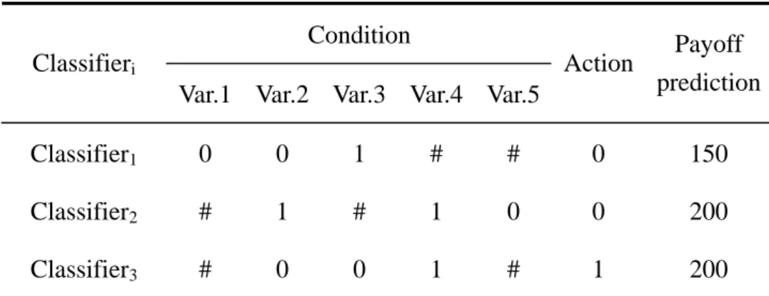
(30) In short, XCS is a learning machine which keeps learning ongoing. In the process of learning, regularities hided from environment are caught by XCS. In other words, it attempts to achieve the direction of generalizing inputs from the environment.. 3.2 Terminology and Notation. 3.2.1 A classifier in XCS. The regularities contained in XCS are called classifiers, which mean knowledge to XCS. They are in the form of condition-action rules defined as follows: <Classifier> ::= <Condition> : <Action> => <Payoff prediction>. There are a condition part, an action part, and a payoff prediction parameter in a classifier. It represents that if the input from environment is fitted in with the condition of a classifier and the action of it is executed by XCS, then an amount of payoff will be expected. The payoff prediction p is the estimation to a classifier’s receivable payoff when condition is matched and action is taken by the system.. In order to reduce the complexity of expressing environment, an input is represented as a string of binary value {0, 1}. Accordingly, the syntax of condition is a string from {0, 1, #}. More than one input can be matched by a condition if it contains #’s [37, 38]. It is explaining as generalization, an important, indeed vital ability for XCS to show regularities of environment compactly [39].. The action chosen by XCS is a discrete value represented as a string. For example, some problems have to be taken as a yes-no decision, then the action of a classifier will therefore be. 20.

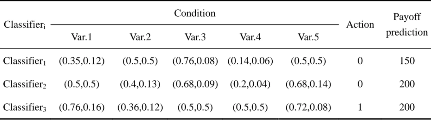
(31) 1 or 0. It is the same as the problem of this paper, to determine a corporation is distress or not. Some classifier examples are showed in Table 3.1.. Table 3.1 Three classifier examples Condition Classifieri. Action. Payoff prediction. Var.1 Var.2 Var.3 Var.4 Var.5 Classifier1. 0. 0. 1. #. #. 0. 150. Classifier2. #. 1. #. 1. 0. 0. 200. Classifier3. #. 0. 0. 1. #. 1. 200. Notes: (1) In this example, there are five variables in the condition of a classifier. (2) E.g. if the classifier1 is satisfied with an input string begins with 001, and action 0 is taken, then a payoff of 150 units will be expected. It is a limitation to use only two values, 1 and 0 (plus #), to represent each individual variable (bit) of the condition [37]. In many environments, the possible value of the variables of interest is continuous, or is perhaps more than two. Obviously, if there exists continuous variables in environment, then the regularities can only accurately caught by chance. Since it is only in fortuitous cases to set the right thresholds to fit the {1, 0, #} coding.. Wilson [40] brought up a new version of XCS, XCSR (XCS taking real inputs), as a solution to the problem. The traditional syntax of the classifier condition, a string from {1, 0, #}, had been changed to a concatenation of “interval predicates”, inti = (ci, si), where ci and si are real values [40]. A real input χ, each variable χ i of the input is a real value, would be matched by the condition if and only if ci - si ≦ χ i ＜ ci + si. for all χ i . Hence ci can be. regarded as a center value of inti and si as a “spread” or delta value relative to ci in inti. In [40], all χ i are restricted to the range (0.0, 1.0). It implies that the “don’t care” symbol, #, can be replaced as: ∀ int i , s.t. ci - si ≈ 0.0 and ci + si ≈ 1.0 . Wilson [40] mentioned that if the data. 21.

(32) ranges in a real problem are known in advance, such scaling implies no loss of generality. Some examples are showed in table 3.2.. Table 3.2 Three examples of classifiers taking real values Condition Action. Payoff prediction. (0.5,0.5). 0. 150. Classifieri Var.1. Var.2. Var.3. Var.4. Var.5. Classifier1. (0.35,0.12). (0.5,0.5). (0.76,0.08) (0.14,0.06). Classifier2. (0.5,0.5). (0.4,0.13). (0.68,0.09). (0.2,0.04). (0.68,0.14). 0. 200. Classifier3. (0.76,0.16). (0.36,0.12). (0.5,0.5). (0.5,0.5). (0.72,0.08). 1. 200. In this paper, all of the used financial ratios are real values. In order to avoid the drawback of the traditional condition encoding and preserve much more information, the model adopted in this paper is XCSR. The following description will focus on XCSR, which just differs from XCS slightly1.. Besides, there are still another two principal parameters in a classifier: (1) prediction. error ε , an average of estimation about the error in the payoff prediction parameter with respect to actual payoffs received; and (2) fitness F, an inverse function of the prediction error. It made a difference between XCS’s definition of fitness and that of traditional classifier systems. The reliability of a classifier in XCS, fitness, is based on the prediction error which is a measure of the accuracy of a classifier’s payoff prediction, rather than originally the prediction itself. Moreover, a niche, instead of a panmictic, genetic algorithm is blended. Consequently, it brings on a strong tendency to evolve classifiers into not only accurate but maximally general ones [39].. 1. The differences between XCSR and XCS are only input interface, mutation operator, and covering [40]. Covering takes place while no existing classifier matches the input. The detail description gives in section 3.3.1. 22.

(33) 3.2.2 The different sets. There are three major sets in XCSR, the same as in XCS, introduced as follows. • All classifiers contained in XCSR are in the population [P]. • The match set [M] is derived from the current [P]. Those that match the current input from the environment are included in [M]. • The action set [A] is derived from the current [M]. All classifiers of [M] that advocate the taken action are included in [A].. 3.3 The framework of XCSR. Two kinds of work, single- and multiple-step tasks, can be solved in the frame of XCS. However, to take the problem of this paper into consideration, it is appropriate to apply XCSR for single-step tasks in which an input is detected, an action is taken, and then some payoffs are received form the environment [40].. XCSR comprises three major components in its frame: performance component,. reinforcement component, discovery component (fig. 3.1). They are separated to give an individual description as follows.. 23.

(34) Discovery Component. Performance Component. The classifiers that match the current input. Population (Covering). Prediction array. Input. Classifier1 … Classifiern. Environment. Match Set. Action Set Action. A place stored system prediction for each action.. The classifiers that match the chosen action. Payoff Reinforcement Component. Figure 3.1 The framework of XCS [3] 3.3.1 Performance component. According to figure 3.1, it is convenient to divide the description of this component into three parts:. 1.. Upon appearance of an input, a match set [M] is formed from the current [P]. Covering occurs if the match set [M] is empty. In this situation, the system creates new classifiers which condition matches the inputχfor each possible action. In XCSR, the new condition has components inti with two possible cases. One is “don’t care”, and the other is ci = χ i and si = rand(s0), where s0 is a constant such as 0.1 and rand chooses a value uniform randomly from [0, s0) [40]. 24.

(35) 2.. For every action i presented in [M], the system prediction Pi, a fitness-weighted average of the payoff prediction p j of each classifier C j in [M], is calculated for each action i.. ∑F p Ρ = ∑F j. Pi is defined as:. j. i. j. , ∀i .. j. j. 3.. An action should be selected in the prediction array where each Pi is placed. The criterion to select an action is according to an explore/exploit regime. This regime is a combination of pure exploration (with probability 0.5 [36]) – deciding the action randomly – and pure exploitation – deciding the best one (the largest Pi). The purpose of this action selection method is to take consideration on making best use of what is learned (exploitation) and also on exploring the solution spaces (exploration).. 4.. While an action is selected in step 3, an action set [A] is formed derived from [M]. All classifiers advocating the chosen action are included. Finally, that action is sent and an amount of payoff is rewarded immediately by the environment.. 3.3.2 Reinforcement component. The function of this component is to update the p , ε , and F parameters of each classifier in [A]. Hence this component acts on [A] in figure 3.1. The reward R returned by the environment is used to update these three parameters in the order: p , ε , and F. The standard Widrow-Hoff delta rule [41] with learning rate β (0< β ≦1) is used for updating these three parameters. However, it is activated only after the number of a classifier has been adjusted. exp is more than or equal to 1 β . This two-state update approach was called “MAM” (“moyenne adaptive modifiée”), introduced in [42]. It makes the early updating procedure quickly to move toward their “true” value, and avoids the system sensitive to beginning, probably arbitrary, setting of the parameters. The following description is given in turn. 25.

(36) 1.. The p of each classifier in [A] is updated as follows: for each classifier C j in [A], p j ← p j + β ( R − p j ) , if exp of C j > 1 β ;. otherwise, p j ← p j + ( R − p j ) exp .. (3-1). (3-1) is a kind of exponential moving average of R, such that a greater weight is distributed to the latest R. This procedure let p be equal to R eventually, which reinforces p to predict the payoff exactly. 2.. The error updating procedure is the same as the payoff prediction update, but not reinforce toward R. It is toward the absolute difference R − p j instead, which is a measure of the classifier’s current error [36]. The update equation is as follows: for each classifier C j in [A], ε j ← ε j + β ( R − p j − ε j ) , if exp of C j > 1 β ; otherwise, p j ← p j + ( R − p j − p j ) exp .. 3.. (3-2). Before updating the fitness of each classifier, the accuracy of its payoff predictions is computed first. The accuracy κ j of each classifier C j is the basis of its fitness F j . It is computed as: for each classifier C j in [A], κ j = 0.1(ε j ε 0 ) − n , if ε j > ε 0 ; otherwise, κ j =1.. (3-3). ε 0 is a threshold under which the accuracy of a classifier is set to 1. Next, the relative accuracy of each classifier κ ′j is computed: κ ′j =. κj . It is an important measure to ∑κ j j. compare the accuracy with other classifiers in [A], instead of with their absolute accuracy. Finally, the fitness F j is updated by using κ ′j in MAM procedure. It is calculated as follows:. 26.

(37) for each classifier C j in [A], F j ← F j + β (κ ′j − F j ) , if exp of C j > 1 β ; otherwise, F j ← F j + (κ ′j − F j ) exp .. (3-4). Consequently, (3-4) shows that the fitness of a classifier is based on its accuracy, relative accuracy actually, as described in section 3.2.1. 3.3.3 Discovery component. In addition to reinforcement learning, discovery component also plays an important role in the process of capturing regularities. The goal of this component is to explore better classifiers and to improve existing ones. It is implemented through a genetic algorithm.. Genetic algorithms (GAs) are stochastic search techniques inspired from natural evolution [43, 44]. In a wide range of applications, GAs have been demonstrated that searching in large and complex spaces is effective and robust [44]. Therefore, GAs are regarded as the way of leading rule discovery in XCS [33].. Figure 3.2 shows the flowchart of a genetic algorithm taken place in the XCSR model. The following is an abbreviated description about it. It is refer to [43, 44] for a more complete description of genetic algorithms.. 27.

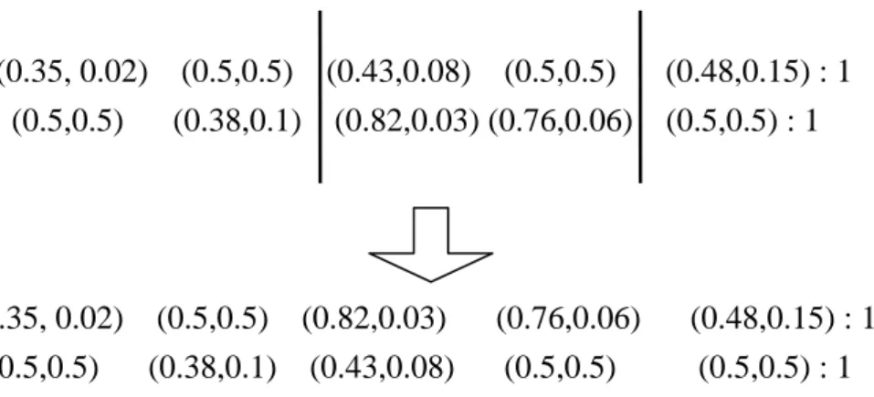
(38) Perform crossover on Ci′. Periodically, a genetic algorithm occurs in [A].. and C ′j with probability χ. Perform two classifiers Ci. Perform mutation on Ci′. and C j selection.. and C ′j with probability µ. Ci and C j are reproduced. Insert Ci′ and C ′j into [P].. to form Ci′ and C ′j . Check for deletion.. Figure 3.2 Flowchart of GAs in XCSR.. In the beginning, a GA is executed in a certain period. The population of the GA is the current action set [A]. That is, the discovery component acts on [A]. Then, two classifiers Ci and C j are selected according to the probability proportional to their fitness and copied to form Ci′ and C ′j . With a high probability χ , also called crossover rate, Ci′ and C ′j are crossed (two-point crossover). Figure 3.3 shows an example.. (0.35, 0.02) (0.5,0.5) (0.43,0.08) (0.5,0.5) (0.48,0.15) : 1 (0.5,0.5) (0.38,0.1) (0.82,0.03) (0.76,0.06) (0.5,0.5) : 1. (0.35, 0.02) (0.5,0.5) (0.82,0.03) (0.5,0.5) (0.38,0.1) (0.43,0.08). (0.76,0.06) (0.5,0.5). (0.48,0.15) : 1 (0.5,0.5) : 1. Figure 3.3 An example of crossover.. 28.

(39) The crossover points, the positions of vertical line in figure 3.3, are randomly selected. The selected parts of Ci′ and C ′j are exchanged with each other to form new ones. The purpose of crossover is to combine two accurate classifiers to yield better ones. In this example, a new classifier is more general than its parents, and the other one is more specific. This situation may not always happen, but it is a tendency toward the balance of generality-specificity [36]. Next, mutation occurs per allele with a very low probability µ (also called mutation rate). It is performed by adding an amount ±rand(m), where m is 0.1 and the sign is chosen uniform randomly. This method was introduced in [40]. The aim of mutation is to introduce innovation to prevent losing some potentially useful genetic material [44]. And then, Ci′ and C ′j are inserted into [P]. If the maximum population size N is reached, two classifiers must be deleted in [P]. The probability of deleting a classifier is confirmed by Kovacs [45]. Low-fitness classifiers that have participated in a threshold number of action sets are preferentially selected to be removed.. It is worth to explain the reason why GA is taken place periodically and the necessity of deletion. It is designed with the aim to keep the resources of the system balanced. Balance means that approximately equal numbers of classifier are allocated to each action set (called niche). Some niches may appear more frequently than others in some environment, so that there are different payoff levels in different niches of the environment. To avoid population full of classifiers in high-payoff niches, it is necessary to balance the active classifiers to share the available payoff [38]. Therefore, it is a niche GA, not a panmictic one, to assist XCSR in discovering more accurate and general classifiers.. 29.

(40) 3.4 Summary. XCS classifier systems are a learning machine exploiting reinforcement learning and evolutionary computation (GAs) to capture regularities from the environment. The developed regularities represent the generalization of inputs for that environment. That is, XCS learns some knowledge about the environment.. The accuracy-based feature makes XCS to discover regularities which are not only accurate but maximal general. These regularities are therefore suitable for prediction and classification. To match the format of this paper’s inputs, financial ratios, the representation of condition in a classifier is an interval for real value. This XCSR model is similar to the original XCS model with extending the representation of inputs.. Consequently, because of the accuracy-based characteristic and the regularities extracted from the environment, this paper would utilize the XCSR model to develop the financial distress prediction model for an accurate result.. 30.

(41) Chapter 4: Research Design. According to the review in previous chapters, several methods were applied to develop the financial distress prediction model but with some drawbacks. XCS classifier systems taking real inputs (XCSR) are a learning machine adequate for prediction described in chapter three. To achieve the purpose of this paper, it therefore implemented the XCSR model with the data from the listed companies in Taiwan. Since logistic regression provides relatively less statistical assumption but more information about the predicted company than NNs, it was then developed with the same data for the comparisons to the XCSR model.. This chapter described the details about the architecture of this paper. It included the selected sample, research limitation, experimental models, and descriptions about the statistical tests.. 31.

(42) 4.1 Research Architecture. The purpose of this paper was to construct XCS classifier systems taking real inputs (XCSR) for the prediction of financial distress and non-distress. The developed XCSR structure was then compared and evaluated against logistic regression model. The architecture of this paper showed in figure 4.1.. Data Pre-Processing. Company Selection. Selection Criteria. Criterion 1 Criterion 2 … Criterion n. Pre-process ratios through scaling.. Sample Matching Make pairs upon industry type and firm size.. Modeling. Modeling by. by XCSR. Logistic Regression. Results Comparison Data Collection Make discussion through. Collect financial ratios as input variables.. comparing results and statistic tests.. Figure 4.1 Research Architecture. From figure 4.1, this paper utilized historically financial ratios as the inputs of models for the prediction of financial distress and non-distress. Companies were selected according to. 32.

(43) different criterion which is the operating definition of this paper. Distressed companies were compared with non-distressed ones preceding the time period in which the distressed event happened. Data were collected using equivalent lead times, and then pre-processed for available in the XCSR model.. The method developed for the prediction was a XCSR model. During the training period, the XCSR model captured the regularities between the financial ratios and distress or non-distress. And this paper utilized the identical financial ratios to formulate the logistic regression model. The XCSR model was then compared to conventional logistic regression model for their obtained results. Finally, the results of two models presented to make some discussion and conclusion.. 4.2 Sample Selection. 4.2.1 Selection Criteria. On the basis of previous studies and domestic circumstances, distressed companies were defined as meeting at least one of the following criteria: • A company applied to the court for pronouncement of its bankruptcy or of reorganization. • Their listed security was placed under altered-trading-method category. • Their listed security is either declared to suspend the trading or to terminate its listing. • Their checks were bounced, or they became refused accounts. • A company applied to someone (often ministry of finance) for mitigating financial. difficulties. • Their money supply is tight by the bank. • Stoppages caused by financial stressed. 33.

(44) For those selected distressed companies, the corresponding non-distressed ones were then matched under industry type and firm size during the same time. The size of a company was determined by its assets. The determination of a company’s industry type was referred to the industrial category announced by Taiwan Institute of Economic Research (TIER). This category used here differs from previous studies. Domestically, prior studies mostly used the industrial category announced by Taiwan Stock Exchange Corporation (TSEC). However, it was quite simpler than the “Standard Industrial Classification System of the Republic of China” published by Directorate-General of Budget, Accounting and Statistics Executive Yuan (DGBAS) in January 2001. In order to avoid mismatching, this paper used the industrial category announced by TIER which provided more detailed industrial classification following DGBAS’s version.. 4.2.2 Experimental Data. 1. Research Scope. This paper used 1999 – 2003 data from Taiwanese listed companies, as reported in TEJ database. The selection and paired criteria were those described in section 4.2.1. On the other hands, it is similar to prior studies that financial institutions are excluded, with the reason that their ratios and cash flows existed substantial differences from those of other types of firms. The final sample, approximately with proportion of 1 distressed to 2 non-distressed firms, included 182 firms (65 distressed and 117 non-distressed). The sample distribution for the distressed and non-distressed firms is summarized in table 4.1.. 34.

(45) Table 4.1 Sample distribution by year Group. 1999. 2000. 2001. 2002. 2003. Total. Distressed. 16. 18. 12. 12. 7. 65. Non-distressed. 29. 33. 21. 23. 11. 117. The distributions for the sample were partitioned into a training set and a testing set. The training data is used with the aim to estimate coefficients in logistic regression model and to capture regularities in XCSR model, and then the testing data is used to measure adaptability of both models. The training sample contained 1999 – 2001 data with 129 companies (46 distressed and 83 non-distressed), and the testing sample consisted of 2002 – 2003 data with 53 companies (19 distressed and 34 non-distressed).. 2. Data Sources. The distressed events of companies were obtained from TSEC monthly review No.442 to No.501 and Securities and Futures Institute (SFI) Online Database. And the sample financial data was collected from Taiwan Economic Journal (TEJ) Database. If there were still inadequate from the above source, plus Market Observation Post System、seasonal reports、 and prospectus as supplements.. 4.2.3 Research variables. Mostly, the preceding researchers used annual financial statement to calculate the ratios. However, the information disclosed in annual reports was much latter than that in seasonal financial statements. Besides, SFC requested the listed companies should publish their financial statements every season. Therefore, this paper used the seasonal financial ratios for 35.

(46) more information, instead of yearly ones. Before introducing the selected ratios in this paper, a timing issue of selecting ratio period mentioned by Ohlson [3] should be discussed.. The time of announcing financial statements was necessary to pay attention to. In Taiwan, the time points of publishing financial statement showed in figure 4.2.. First season. Second season. Third season. Fourth season. Fiscal. Fiscal. year-start date. year-end date. 4/30 1/1. 3/31. 8/31 6/30. 10/31 9/30. 12/31. Both the annual report prior to. The second. The third. this year and the first seasonal. seasonal report. seasonal report. report are announced.. is announced.. is announced.. Figure 4.2 the time point of announcing financial statement [46]. Previous studies seemed implicitly to consider the timing issue. Studies using annual reports were to give an example. From figure 4.2, the annual data is reported next March. It seemed that these studies, but by no means all, presume that a financial statement is available at the fiscal year-end date. However, it is possible that a distressed event took place at the time point after the fiscal year date, but prior to announcing the financial statements. This was the problem Ohlson [3] addressed which may lead to “back-casting” for many of the distressed companies.. In order to avoid this problem, the selected period of every distressed firm was designed as figure 4.3. 36.

(47) Eight seasons. TN -7 (3). TN (2). Toe (1). Figure 4.3 Time point selection Notes: (1) Toe represents the occurrence of financial-distressed event. (2) TN represents the nearest financial statement announcements prior to Toe. (3) TN -7 represents the time point eight seasons prior to TN. According to figure 4.2, while a distressed event of a company took place at the time Toe, the nearest time point of announcing financial statements prior to Toe , TN , was then determined. For example, if a distressed event of a company arose at the middle of July (Toe), then TN should be April which indicated the second seasonal report instead of the third one. After determining TN, the corresponding seasonal report was also determined. Then the data period was between TN and the time point TN -7 seven seasons priori to TN. In other words, this paper used the financial ratios of each distressed company calculated from TN -7 to TN (i.e., total 8 seasons) and used the same period for the paired non-distressed companies.. According to section 2.3, the framework announced by SFC was the basic structure for this paper’s input variables. In addition to this, the selected ratios were also considered on the basis of their performance in prior studies. In other words, this paper has taken practical and empirical considerations on choosing explanatory variables. Table 4.2 listed these selected ratios in this paper.. 37.

(48) Table 4.2 Selected variables [47] Category. Variable. Formula. current Assets Current Liabilities. Current Ratio. Liquidity Construct. Quick Assets Current Liabilities. Quick Ratio. Quick assets = current assets inventory. Working Capital to Total Assets Ratio. Working Capital Total Assets. 38. Description • This ratio evaluates an enterprise’s short-term debt-paying ability and overall liquidity position. • The higher this ratio, the less probability a company becomes financially distressed. • In addition to current ratio, it is prefer to examine a more immediate liquidity position at times. That is, quick ratio. • The usual guideline of this ratio is larger than 1.00. • This ratio measure a company’s liquidity relative to the total capitalization. A shrink of this ratio often represents an operating loss of the firm..

(49) Table 4.2 Continued Category. Variable. Times Interest Earned. Capital Structure Construct. Cash Flow Construct. Formula After − tax Net Income, plus Interest Expense, and Income Tax Expense Interest Expense. Total Liabilites Total Assets. Debt Ratio. Description • This ratio evaluates a company’s ability to pay the interest expense by net income. That is, the level of meeting its interest obligations. • This ratio measures how well creditors are protected in case of insolvency. • The higher this ratio, the worse the company’s position.. Permanent Capital To Fixed Assets Ratio. Equity + long - term debt Fixed Assets. • This ratio determines how well the fitness between capital structure and assets structure.. Fixed Assets to Total Assets Ratio. Fixed Assets Total Assets. • This ratio determines how well the fitness between fixed assets and assets structure.. Cash Flow from operations Current Liabilites. Cash Flow Ratio. 39. • This ratio evaluates the payback ability to meet short-term debt by generating resources..

(50) Table 4.2 Continued Category. Variable. Formula. Inventory Turnover. Accounts Receivable Turnover. Cost of Goods Sold Average Inventory. • This ratio determines the liquidity of the inventory, which helps to understand the managing performance of inventory.. Net Sales Average Gross Receivables. • This ratio evaluates the liquidity of the receivables, which helps to make decisions about extending sales.. Net Sales Average Total Assets. • This ratio determines the activity of the total assets and also the ability of the company to generate sales through utilizing the total assets.. Net Sales Average Fixed Assets. • This ratio measures the activity of the fixed assets and the ability of the firm to generate sales through the use of the fixed assets.. Operation Performance Construct Total Asset Turnover. Fixed Asset Turnover. 40. Description.

(51) Table 4.2 Continued Category. Variable. Formula. Net Income to Sales Ratio. Net Income Net Sales. After-Tax Return On Assets. After - Tax Net Income Average Total Assets. • This ratio evaluates the ability of the firm to create profits through utilizing its assets.. After-Tax Return On Equity. After - Tax Net Income Average Total Equity. • This ratio measures the firm’s ability to generate return to the shareholders.. Gross Profit Margin. Gross Profit Net Sales. • This ratio evaluates the ability of the firm to produce a good or service at a low cost or a high price.. Sales Growth Ratio. Net Sales t − Net Sales t -1 Net Sales t -1. Profitability construct. Growth construct After Tax Net Incomet. After-Tax Net Income Growth Ratio. − After Tax Net Incomet -1 After Tax Net Incomet -1. 41. Description • This ratio measures the profitability of the company.. • This ratio measures a firm’s degree of growth for the net sales after tax. • This ratio measures a firm’s degree of growth for the net income after tax..

(52) These ratio data was required to be pre-processed for the usage of XCSR. The pre-processing procedure used the following formula:. χ i, j ' =. χ i , j − min j max j − min j. , ∀1 ≤ i ≤ m,1 ≤ j ≤ n. (4-1). Where:. χ i, j : The ith record of jth ratio χ i , j ' : The processed value of χ i , j min j : The minimum of jth ratio max j : The maximum of jth ratio m: The total number of record in data n: The total number of financial ratios (4-1) involved mapping each ratio to a range with minimum and maximum values of 0.0 to 1.0, respectively. For the transformed format, it would suit for the inputs of the XCSR model.. 4.3 Research limitation. It did not include all the practically influenced variables for the likelihood of financial distress in this paper. Some restrictions of this paper are given as follows: • Sample limitation: This paper used only listed companies with the reason that their. financial data is much more confidence than the unlisted companies. The selected sample is therefore with the restriction on the listed companies. • Accounting limitation: The financial ratios used in this paper were calculated from the. financial statements. There may take place bias among the company’s ratios because of 42.

(53) the differently calculated methods under generally accepted accounting principles. It is an unavoidable restriction. • Data limitation: This paper only used the quantitative data. That is, the financial ratios. For. other qualitative variables are not in the considered range.. 4.4 Implementation Models. 4.4.1 XCSR Model. This paper implemented Wilson’s [40] XCSR model with almost the same structure (see figure 3.1). The input in this paper was the pre-processed financial ratio, and the corresponding taken action was the predicted result. The form of a classifier was similar to that in table 3.2. With regard to every input (a financial ratio) from environment, XCSR will chose the suitable classifiers to take an action (to predict distressed or non-distressed). If it predicts correctly, the environment will reinforce those in action set with positive payoff; otherwise with -100. Finally, the classification accuracy was calculated to compare with that of logistic regression model. For the comparison with fair, those inputs caused the mechanism of covering, not been predicted by XCSR, were excluded in calculating the accuracy.. The major parameters in the XCSR model listed below, additional information about XCSR referred to chapter three. • N, the maximum size of the population, equals 400. • β , the learning rate for p , ε , and F, equals 0.4. • ε 0 and n, used to compute the fitness of a classifier, are 10 and 5. • θ GA , the threshold to determine whether GA can take place, equals 15.. 43.

(54) • χ , the crossover rate, equals 0.8. • µ , the mutation rate, equals 0.05. • P#, the probability of using a don’t-care in one variable in a classifier when covering,. equals 0.8. • R, the payoff returned by the environment, equals 1000 for the correct action; -100. otherwise.. 4.4.2 Logistic Regression Model. Previous studies often used logistic regression model with the main reason that it has less statistical assumptions than MDA and linear regression model to deal with dichotomous variables. Additionally, it could handle nonlinear variables and transform the value of the dependent variable into probability which was meaningful to users. Therefore, this paper used logistic regression model as the benchmark compared with XCSR.. The logistic regression gives the equation as follows: n. yi = β 0 + ∑ β j χ i , j + µ i , *. j =1. yi=. 1 if yi* > 0 0 otherwise. (4-2). Where: yi*: The estimated (latent) variable yi : The observed variable representing whether the ith company is distressed (yi = 1) or not (yi = 0). χ i, j : The jth financial ratio of the ith company (total j ratios) β j : The estimated coefficient of χ i, j ( β 0 is the estimated intercept) µi : The error term In (4-2), the conditional probability of yi was then transferred as: 44.

(55) n ⎤ ⎡ Ρ( yi = 1 | χ i , j , j = 1L n) = Ρ ⎢ µi ≤ ( β 0 + ∑ β j χ i , j )⎥ j =1 ⎦ ⎣ n ⎡ ⎤ 1 = F ⎢β 0 + ∑ β j χ i, j ⎥ = n −( β 0 + ∑ β j χ i , j ) j =1 ⎣ ⎦ j =1 1+ e. (4-3). In (4-3), the cumulative distribution function of µi (function F) is assumed as a logit function. For this reason, these independent variables (financial ratios) could be transformed to an estimated probability fell into a range between 0.0 and 1.0. This paper used a cutoff value equaling 0.5 as a threshold of the prediction. In other words, the model determined a company as distressed while its estimated probability is greater than 0.5, otherwise determined it as non-distressed. Moreover, the stepwise procedure was used to determine the significantly explanatory variables. The criterion for entering and removing variables in the model was a 0.10 and a 0.15 probability level, respectively.. 4.5 Statistical Test Description. The purpose of using statistical tests is to prove the significance of the predictive results. The tests were done in three parts: classification accuracy test, differences between two models’ accuracy test, and tendency test. The descriptions for individual test were given bellow.. 1. Description of Test for Classification Accuracy. In order to evaluate the accurate level both models achieved, a statistical test introduced by Huberty [48] was used. He proposed a test statistic Z* which follow an approximately normal probability distribution, for assessing the statistical significance of the classification rate is given by 45.