應用於H.264可調式視訊串流之前向糾錯—失真最佳化演算法

國

立

交

通

大

學

多媒體工程研究所

碩

士

論

文

應用於 H.264 可調式視訊串流之動態前向糾錯—失

真

最

佳

化

演

算

法

Dynamic FEC-Distortion Optimization for H.264 Scalable Video

Streaming

研 究 生：溫維中

指導教授：蕭旭峰 教授

摘要

Abstract

Forward error correction codes have been shown to be a feasible solution either in

application layer or in link layer to fulfill the need of Quality of Service for multimedia

streaming over the fluctuant channels. In this paper, we propose the Dynamic FEC-distortion

optimization algorithm to efficiently utilize the bandwidth for better video quality. The

optimization criterions are based on the unequal error protection by taking account of the

error drifting problems from both temporal motion compensation and inter-layer prediction of

H.264/MPEG-4 AVC scalable video coding. Also, it can adapt to the content-dependent

quality contribution of each video frame in a video layer. Lightweight error-concealment is

Acknowledgement

Contents

摘要...I

ABSTRACT ... II ACKNOWLEDGEMENT ... III CONTENTS ...IV LIST OF TABLES ...VI LIST OF FIGURES... VII

I. INTRODUCTION ... 1

II. SCALABLE VIDEO CODING ... 3

-2.1H.264/MPEG-4AVCSCALABLE EXTENSION...-3-

2.2MOTION PREDICTION...-4-

2.3ERROR CONCEALMENT TOOL...-5-

III. FECDISTORTION OPTIMIZATION ALGORITHMS... 8

-3.1FORWARD ERROR CORRECTION CODES...-8-

3.1.1 ReedSolomon code... 9

3.1.2 How to generate a systematic ReedSolomon erasure code... 9

3.1.3 Encoding and decoding of systematic ReedSolomon codes ... 10

-3.2BERKELEY ALGORITHM...-10-

3.2.1 Component ... 10

3.2.2 Distortion... 11

3.2.3 Algorithm... 12

3.2.4 Problem when applying to H.264 SVC... 13

-3.3FLAT FEC-DISTORTION OPTIMIZATION ALGORITHM...-16-

3.3.1 Algorithm... 16

3.3.2 How to determine the α factor ... 18

3.3.3 Packetization ... 22

-3.4DYNAMIC FEC-DISTORTION OPTIMIZATION ALGORITHM...-24-

3.4.1 Classifying Pictures to Clusters ... 25

3.4.2 Protecting Scheme... 25

3.4.3 Algorithm... 26

3.4.4 How to determine β factor... 29

4.1.1 Environment... 32

4.1.2 Simulation Results ... 33

-4.2SIMULATIONS FOR DYNAMIC FEC-DISTORTION OPTIMIZATION...-36-

4.2.1 Environment... 36

4.2.2 Simulation Results ... 40

V. CONCLUSION... 46

-List of Tables

Table 3-1 An example of picture sizes of a GOP……….. 15

Table 3-2 Encoding parameters and PSNRs……….. 17

Table 3-3 Experiment data………. 21

Table 3-4 Protection results………... 23

Table 3-5 Encoding parameters and PSNRs……….. 30

Table 4-1 Encoding parameters and PSNRs……….. 32

Table 4-2 Protection results………... 33

Table 4-3 Encoding parameters and PSNR……….. 37

Table 4-4 Encoding parameters and PSNR………... 39

List of Figures

Fig 2-1 Basic coder structure for the scalable extension of H.264/MPEG-4 AVC… 4

Fig 2-2 Hierarchical-B motion prediction……….. 5

Fig 2-3a Case 1: Error concealment when a non-base layer is lost………. 6

Fig 2-3b Case 2: Error concealment when a base layer is lost……… 7

Fig 3-1 The Vandermonde matrix used in our FEC code……….. 10

Fig 3-2 Component……… 11

Fig 3-3 Rate-Distortion curve……… 12

Fig 3-4 Packet lengths……… 14

Fig 3-5 Partially received layer may contribute PSNR……….. 18

Fig 3-6 PacketLossRate-Alpha curve……… 20

Fig 3-7a Alpha-PSNR curves of video “mobile” ………... 20

Fig 3-7b Alpha-PSNR curves of video “crew” ………... 21

Fig 3-8 An example of picture classification………. 25

Fig 3-9 An example of DFDO protecting scheme………. 26

Fig 3-10 A binary tree for 3-layer video……….. 28

Fig 3-11a Beta-PSNR curve for video sequence “ice” ………. 30

Fig 3-11b Beta-PSNR curve for video sequence “city” ……… 31

Fig 4-1 Given bandwidth………... 33

Fig 4-2 Simulation results different packet loss rates……… 35

Fig 4-3 Simulation results different packet loss rates……… 36

Fig 4-4a Given bandwidth………... 37

Fig 4-4b Given bandwidth………... 37

Fig 4-5a Given bandwidth………... 38

Fig 4-5b Given bandwidth………... 38

Fig 4-6a Simulation result of FFDO……… 42

Fig 4-6b Simulation result of DFDO………... 42

Fig 4-6c The difference of simulation results……….. 43

Fig 4-6d The difference of simulation results……….. 43

Fig 4-7a Simulation result @ 15 fps……… 44

Fig 4-7b Simulation result @ 15 fps……… 44

Fig 4-8 Simulation result with different packet loss rate………... 45

I. Introduction

Personal, home, or handheld entertainment systems, such as DVB-H [1] and IPTV which is under construction to be a standard by ITU-T, have been an emerging research and industrial emphasis due to the great progress of the network communications and joint multimedia/channel coding technologies. It is rather challenging to fulfill the needs for Quality of Service and Quality of Experience requirements in the mobile environments of such entertainment systems that might suffer from dynamic channel fluctuation.

Besides Automatic Repeat reQuest (ARQ) which possibly suffers from the intolerable end-to-end packet delay and exacerbated jitter, forward error correction codes have been shown to be a feasible solution. In DVB-H, Multi-Protocol Encapsulated Forward Error Correction (MPE-FEC) is used by interleaving the information packet and the protection packets from Reed-Solomon code to deal with the burst error. The error protection strength in MPE-FEC is not really content-dependent. Besides Reed-Solomon code, rateless erasure codes (also known as fountain code [2]), such as raptor code [3], provide virtually infinite protection symbols and the modified version of such code has been recently adopted in 3GPP [4]. However, unlike Reed-Solomon error erasure code which shows maximum distance separable property, fountain codes generally have less coding efficiency.

In [5], Tan et al. proposed layered FEC for sub-band coded scalable video multicast using equation-based rate control while adaptive FEC is adopted to recover the lost packets so that the distortion function can be minimized with the optimized subscription of video and FEC layers, under an assumption that different frames in a video layer shall have the same distortion.

maximize the streaming throughput while maintaining an upper bound of the error rate for each scalable video layer that FEC fails to decode. However, the upper bounds are pre-set without further explanation.

The impact of packet loss and FEC overhead on scalable bit-plane coded video in best-effort networks is analyzed in [7] and a similar optimization algorithm was proposed to allocate the bandwidth resource to FEC and video data.

In this paper, we propose FEC-Distortion optimization algorithms that take account of the error drifting problems from both temporal motion compensation and inter-layer prediction of H.264/MPEG-4 AVC scalable video coding, as well as the content-dependent visual quality contribution of each video frame in a video layer to achieve better quality of service with the same resource. In case of occasional packet error that is not recoverable by the FEC scheme, lightweight error-concealment is also incorporated with the proposed algorithms for better quality of reconstructed video.

The rest of this paper is organized as follows. In Chapter II we introduce the scalable video coding and the error concealment tool we added in the reference software. In chapter III we describe predecessor’s work on the same topic as well as our two FEC optimization algorithms, Flat FEC-Distortion Optimization and Dynamic FEC-Distortion Optimization, to be used with H.264 scalable video coding, followed by Chapter IV, the simulation results and discussions. The concluding remarks are presented in Chapter V.

II. Scalable Video Coding

Traditional video coding techniques, such as waveform-based and content-dependent

methods [14], aim to optimize the coding efficiency at a fix bit rate, and this presents a

difficulty when multiple users try to access the same video through different communication

links. [14] For example, a video encoded at 1.5 mbps can be downloaded and played at real

time via a high-speed link, such as ADSL. But for users with only a modem connection at 56

kbps, it is not possible to receive sufficient bits for real-time play. [14] In such cases, the same

video needs to be encoded at different bit rates to fulfill a range of users’ abilities.

Usually, a scalable video codec (SVC) provides scalability on SNR, spatial, temporal, or

any combination of them, in a single encoded video stream. High-speed link users can choose

to download the entire stream to have the best video experience, and for users with low-speed

or low computation power environment, they can download partial of the same stream.

2.1 H.264/MPEG-4 AVC Scalable Extension

H.264/MPEG-4 AVC scalable extension is a standard developed jointly by ITU-T and

ISO. These two groups created the Joint Video Team (JVT) to develop the H.264/MPEG-4

standard which has features such as hierarchical prediction structure, usage and extension of

the network abstraction layer (NAL) unit concept of H.264/MPEG-4 AVC, and fine granular

only can encode/decode videos according to the H.264 SVC standard but also provides a

toolset to down-sample/up-sample contents and calculate PSNR.

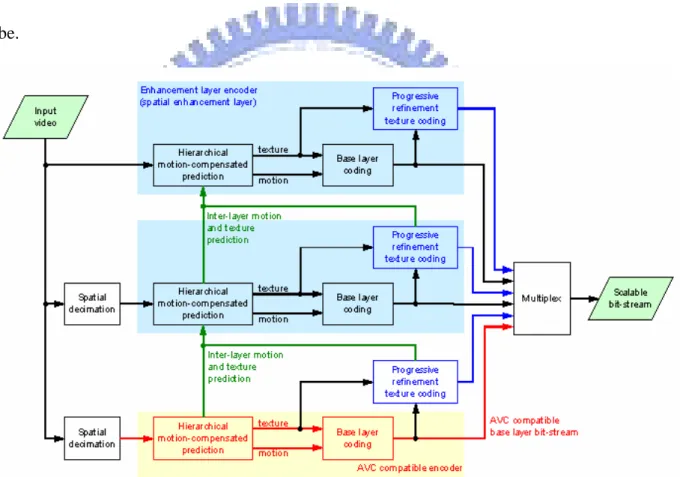
Figure 2-1 shows the basic structure of H.264 SVC, where the base layer is AVC

compatible and the other layers provide scalabilities such as SNR, spatial, and temporal. In

the decoder side, in order to decode a picture of higher layer, all the data of lower layers of the

same picture are required. The more the video layers received, the better the video quality will

be.

Fig 2-1: Basic coder structure for the scalable extension of H.264/MPEG-4 AVC [13]

2.2 Motion Prediction

In video coding, motion compensation is a technique used to improve coding efficiency.

Since a video is composed by a series of continuous pictures and neighborhood pictures are

later one. By encoding the difference between the prediction picture and the actual one, there

usually will be a large range of 0s in the residual picture, and the number of bits can be further

reduced by run-length coding and entropy coding. A picture is called I-picture or intra-coded

if it needs no reference picture; a picture is called P-picture or inter-coded if it needs reference

picture. B-picture is a special case of P-picture. A B-picture can use up to two reconstructed

pictures as its prediction.

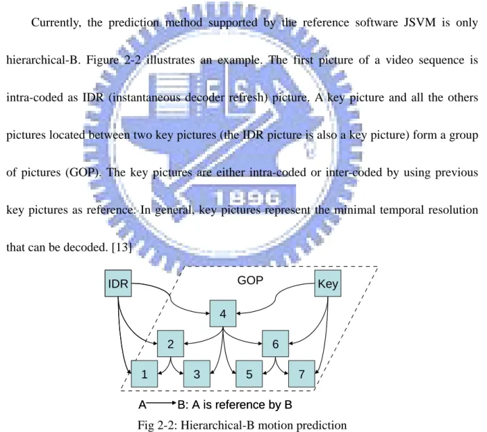
Currently, the prediction method supported by the reference software JSVM is only

hierarchical-B. Figure 2-2 illustrates an example. The first picture of a video sequence is

intra-coded as IDR (instantaneous decoder refresh) picture. A key picture and all the others

pictures located between two key pictures (the IDR picture is also a key picture) form a group

of pictures (GOP). The key pictures are either intra-coded or inter-coded by using previous

key pictures as reference. In general, key pictures represent the minimal temporal resolution

that can be decoded. [13]

IDR 1 2 3 4 5 6 7 Key GOP A B: A is reference by B IDR 1 2 3 4 5 6 7 Key GOP A B: A is reference by B

Fig 2-2: Hierarchical-B motion prediction

to moderate the quality degradation when a video stream can’t be fully received. Error

resilient means this function is provided by encoder, such as including some extra headers in

stream to help the detection of lost information, or simple duplication of encoded frames. In

contrast, error concealment is implemented at the decoder side only.

When a scalable layer of a picture is lost, the decoder in the reference software JSVM

may either crashes or skips the entire picture. However, even if the decoder doesn’t crash, the

decoded video still suffers from the error propagation and the visual quality dramatically

decreases. In our implementation of error concealment, we fix this problem by frame

duplication and interpolation. Thus, further reference to this lost frame can be found and the

quality degradation caused by reference error is moderated.

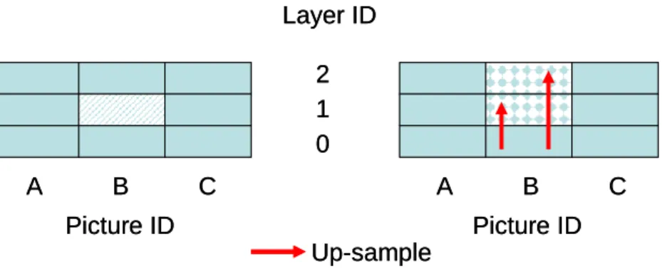
Figure 2-3a and 2-3b illustrate two examples of how the error concealment tool works

when picture loss occurs. When a non-base layer is lost, decoder uses the reconstructed frame

of its lower layer as its replacement. On the other hand, if the base layer of a picture is lost,

decoder replaces the lost frame with the reconstructed base layer of nearest picture along the

time axis, and then resamples the replacement to proper resolution.

Layer ID 0 1 2 Picture ID Picture ID A B C A B C Up-sample Layer ID 0 1 2 Picture ID Picture ID A B C A B C Up-sample

Layer ID 0 1 2 Picture ID Picture ID A B C A B C Up-sample Frame copy Layer ID 0 1 2 Picture ID Picture ID A B C A B C Up-sample Frame copy

III. FEC-Distortion Optimization Algorithms

In this chapter, we will briefly introduce forward error correction code and then describe

the algorithm proposed by Tan et al. in [5] as well as ours. When applied to a scalable video

stream, these algorithms choose a subscription – which records how many video layers or

clusters of video data to be protected and the corresponding protection strength so that the

minimal distortion for each GOP can be approached. We also describe the modified version of

[5] to apply Tan’s algorithm to the scalable extension of H.264/AVC codec, which is denoted

as Flat FEC-Distortion Optimization algorithm described in Section 3.3.

3.1 Forward Error Correction Codes

Forward error correction (FEC) code is a technique used to protect data through

transmission. The advantage of using FEC code over Automatic Repeat reQuest (ARQ) on the

multimedia streaming is that it can avoid the retransmission of lost data which will increase

the total delay and is not feasible in real-time play situations such as live shows or video

conferences.

Different types of FEC codes have different properties and error-correction abilities. An

error detection/correction code recovers information by two steps. First, it detects whether if

error occurs and the location of errors. And then it tries to correct the corruption. On the other

information as long as the number of received encoded information exceeds a predefined

threshold. We use error erasure codes because in the case of transmitting video streams,

receivers know which packets are lost. All the algorithms described in later sections use one

of the most famous systematic erasure codes, Reed-Solomon code [10], to protect video

streams. The term “systematic” means that the information data is part of the encoded data.

3.1.1 Reed-Solomon code

Reed-Solomon code was introduced by I.S. Reed and G. Solomonand. It is widely used

in data storage, data transmission, mail encoding, and satellite transmission. The minimal data

unit in Reed-Solomon codes is symbol, which may consist of one or more bits. Before

encoding, information will be divided into some message blocks which consist of a

predetermined number of symbols. In a Reed-Solomon erasure code with parameter pair (N,

K), a message block consists of K source symbols and is protected by generated N-K

protecting symbols. At receiver side, it can recover information as long as there are more than

or equal to K received encoded symbols.

3.1.2 How to generate a systematic Reed-Solomon erasure code

We use the FEC code provided in [10] as our systematic Reed-Solomon erasure code. It

uses Vandermonde matrix [16] to construct the generating matrix G, which is used to encode

the source information as well as to decode the protected message blocks. Building generating

codes due to matrix inversion and matrix-vector multiplication [16,17].

The (i,j) element of generating matrix of Vandermonde in [10] can be formed as shown

in figure 3-1, where the xi’s are elements of GF(pr), p is a prime and r is the number of bits in

a symbol. For more detail information about Reed-Solomon erasure code and Vandermonde

matrix, please refer to [12,15,16,17].

1 −

=

x

g

Fig 3-1: The Vandermonde matrix used in our FEC code

3.1.3 Encoding and decoding of systematic Reed-Solomon codes

Before encoding, source information needs to be divided into a number of message

blocks, which consist of a predefined number of symbols that can be recognized by

Reed-Solomon code. A message block is encoded by multiplying it with the generating matrix,

and a protected message block can be decoded by multiplying it with the inverse of the

generating matrix.

3.2 Berkeley Algorithm

3.2.1 Component

The video codec used in [5] is 3D-wavelet sub-band coding, where each sub-band of a

picture will be divided into N coefficient blocks of equal sizes and a component is formed by

grouping coefficient blocks from different sub-bands. As illustrated in figure 3-1, there are

seven sub-bands and each is divided into nine equal sizes coefficient blocks. Then, a

sub-band.

A GOP (group of pictures) can be divided into M components, and each component

consists of many video layers, where each video layer has different playing rate. Thus, spatial

and temporal scalabilities are constituted.

Components are independently decodable because they are independently variable length

coded. Besides, since a component is formed by different spatial locations of coefficient

blocks, the distortion of losing any component can be assumed to be equal.

Fig 3-2 [8]: A component is formed by grouping a coefficient block of different spatial location from each sub-band.

3.2.2 Distortion

The estimation of distortion comes from a pre-measured Rate-Distortion curve, as

Fig 3-3 [8]: Rate-Distortion curve.

3.2.3 Algorithm

By giving available bandwidth and packet lost rate, the proposed algorithm of Tan et al.

chooses a subscription that has the minimal distortion to determine the number of video layers

to be protected and the protection strength for each layer. Equation (1) describes the main idea.

In order to find the best subscription S*, the function D(s,p) is used to estimate distortion of

current GOP when applying subscription s and packet lost rate p. R(s) is the bandwidth used

by applying subscription s and must be less than or equal to the available bandwidth B. M is

the set of all possible subscriptions under B. The final version of distortion function used in (1)

is (4), which is derived from (2) and (3).

Since components of the same layer of a GOP are independently decodable and have

similar importance, the distortion of a GOP is about to be the sum of distortions of all

components of all subscribed layers. Thus, equation (2) is formed. In (2), M is the number of

components, L is the number of subscribed layers, pi(c) means the decodable probability of the

by rate-distortion curve mentioned above.

Again, since all components are similarly important, Tan et al. assumes that distortions of

all components are the same, thus equation (3) can be derived from (2). And by defining Di =

MDi(1), equation (4) can be derived from (3), and is the final version of distortion function

used in (1).

In equation (6), qi(c) is the probability that a lost packet of component c of layer i is

unrecoverable. The decodable probability of the only first i layers, pi(c), is illustrated as (5).

By the definition of Reed-Solomon code, when using parameter pair (N, K), there must be

more than or equal to K out of N symbols received to recover all source symbols.

D(s,p)

S

*

arg

min

=

₍₁₎

∑∑

∑

⋅

=

≈

D

p

D

D(s,p)

(2)

∑

(3)

∑

(4)

(

)

(

)

⎪

⎩

⎪

⎨

⎧

=

−

<

≤

−

=

∏

∏

L

i

if

q

L

i

if

q

q

p

1

0

1

(5)

(

)

⎥

⎥

⎦

⎤

⎢

⎢

⎣

⎡

−

⎟⎟

⎠

⎞

⎜⎜

⎝

⎛

+

−

⋅

=

_∑

1

1

p

p

w

k

M

p

q

₍₆₎

3.2.4 Problem when applying to H.264 SVC

faces a problem of packet length. In [5], each packet contains one component and the

components of the same layer are supposed to be of similar sizes. But in the case of the

scalable extension of H.264/AVC, the NAL sizes may vary in a large range, and this causes

problem.

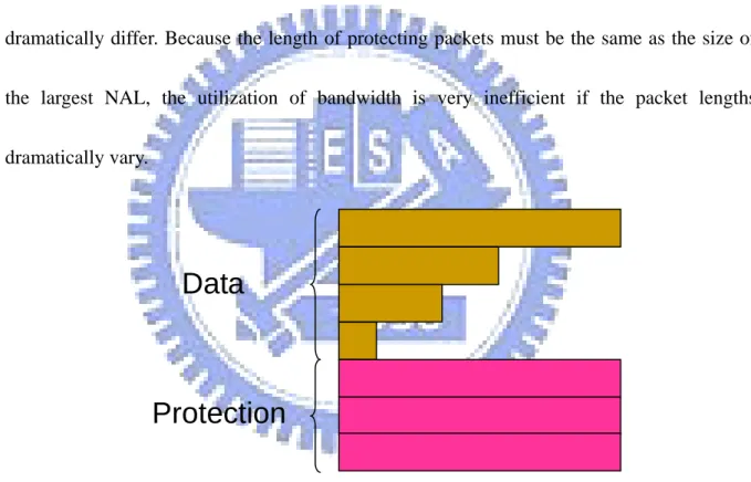
As shown in figure 3-4, where each row is a packet, since NALs may have different sizes,

the packet lengths also differ. The problem occurs when the largest and smallest NAL sizes

dramatically differ. Because the length of protecting packets must be the same as the size of

the largest NAL, the utilization of bandwidth is very inefficient if the packet lengths

dramatically vary.

Data

Protection

Fig 3-4: The length of protecting packets must be the same as the largest data packet Table 3-1 is an example of NAL sizes which are extracted from an actually encoded video

stream and the GOP size is 16. The red and bold numbers are the largest NAL sizes in

corresponding video layers, and the blue and bold are smallest ones. We can observe that the

Table 3-1: An example of picture sizes of a GOP

Picture ID Size (Byte) in 0th layer Size (Byte) in 1st layer Size (Byte) in 2nd layer

1 92 150 125 2 186 255 260 3 100 165 112 4 602 618 411 5 98 194 172 6 222 366 291 7 107 199 151 8 896 819 570 9 103 176 142 10 250 364 245 11 129 200 166 12 532 608 427 13 112 177 171 14 226 312 245 15 101 151 152 16 3034 4582 2962

3.3 Flat FEC-Distortion Optimization Algorithm

In [5], Tan et al. proposed a layered FEC algorithm for sub-band coded scalable video

multicast using equation-based rate control such that packet loss is one of the parameters to

regulate the sending rate while adaptive FEC is adopted to recover the lost packets so that the

distortion can be minimized with optimized subscription S* as described in (1) and (4), under

an assumption that different frames in a video layer shall have the same distortion measure.

Instead of the sub-band scalable video coding with layered structure on both video and

FEC data in [5], our proposed FEC optimization algorithms are based on the H.264/MPEG-4

AVC scalable extension, which is an amendment to the H.264/MPEG-4 AVC standard and it

is scheduled to be finalized in 2007. The base layer of a Scalable Video Coding (SVC)

bit-stream is usually coded in compliance with H.264 while new scalable tools are added for

supporting spatial, SNR, and temporal scalability [9].

When applying to the scalable extension of H.264/AVC, the algorithm in [5] does not

take the effect of reference pictures into account. That means, when a layer of a picture is lost

and can’t be recovered by FEC, the distortion of other pictures which reference the lost one

would increase due to reference error, but in [5] this is not represented. In addition, [5] has the

problem of inefficient bandwidth using as described in Section 3.2.4.

3.3.1 Algorithm

and (2) from [5]: selecting a subscription that not only fits the available bandwidth but also

has the maximal PSNR to determine the number of video layers to be protected and the

protecting strength for each video layer. In contrast with [5], FFDO estimates the PSNR of a GOP of layers instead of PSNR of individual pictures. A factor α is added to the distortion

measuring function to reflect the quality degradation caused by partially received video layer.

The PSNR of a GOP is the summation of PSNR of all subscribed layers. Equation (8)

illustrates the contribution measuring function, where pi is the FEC decodable probability of

only the first i layers, Di is the corresponding PSNR and L is the number of subscribed layers.

The leaky factor α in (9) is a real value between 0 and 1, and is used to represent the PSNR

contributed by the partially received higher layers.

(s,p)

S

*

arg

max

PSNR

=

(7)

∑

(8)

(

)

,

0

1

+

×

−

≤

<

=

α

α

PSNR

PSNR

PSNR

D

(9)

Use fig 3-5 to explain the leaky factor α, where the arrows indicate the reference

relationships. In our implementation of error concealment tool, when a layer of picture is

unavailable, decoder will take the reconstructed picture of lower layer to substitute the lost

one and the further higher layers. In fig 3-5, since the lost NAL belongs to a picture which

will not be referenced by any other pictures,the PSNR contribution of this video layer should

picture. 0 1 2 0 1 2 Picture ID La y e r I D Received Error concealed Lost 0 1 2 0 1 2 Picture ID La y e r I D Received Error concealed Lost

Fig 3-5: Partially received layer may contribute PSNR

Though the definitions of pi in FFDO and [5] are the same, the definitions of qi in both

algorithms are different. In FFDO, qi is the FEC undecodable probability of layer i, as

illustrated in (11), where the protecting parameter (N, K) of layer i is (M + ki, M).

(

)

(

)

∏

∏

(10)

(

)

∑

−

⎟⎟

⎠

⎞

⎜⎜

⎝

⎛

+

=

1

p

p

w

k

M

q

(11)

Sequence Parameter Set Network Abstraction Layer (NAL) units and Picture Parameter

Set NAL units [11] have essential header information in order to decode the video properly

and they are assigned strongest error correction code (n=256).

3.3.2 How to determine the α factor

The α factor in (9) embraces the video quality degradation caused by both partially

received layer data and reference errors, and is too complex and time-consuming to estimate the accurate value of α from all picture layer lost cases in a GOP. Hence, we select α by

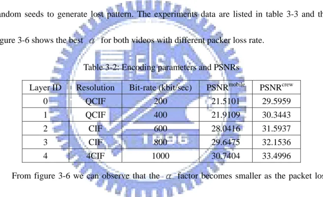
We do experiments on two testing sequences, mobile and crew, with same environment parameters to see the variation tendency of best α when the packet lost rate varies from 0.12

to 0.48. The encoding parameters and the PSNR are listed in table 3-2, where the PSNRs are

calculated by the source video and the up-sampled reconstructed layers. For each given packet loss rate, α is set from 0 to 0.9 to generate the protected video streams. Each protected

stream passes 100 lossy channels which have the same specified packet loss rate but different

random seeds to generate lost pattern. The experiments data are listed in table 3-3 and the figure 3-6 shows the best α for both videos with different packer loss rate.

Table 3-2: Encoding parameters and PSNRs

Layer ID Resolution Bit-rate (kbit/sec) PSNRmobile PSNRcrew

0 QCIF 200 21.5101 29.5959

1 QCIF 400 21.9109 30.3443

2 CIF 600 28.0416 31.5937

3 CIF 800 29.6475 32.1536

4 4CIF 1000 30.7404 33.4996

From figure 3-6 we can observe that the α factor becomes smaller as the packet loss

rate increases. This is reasonable because the partially received layers lost more picture data

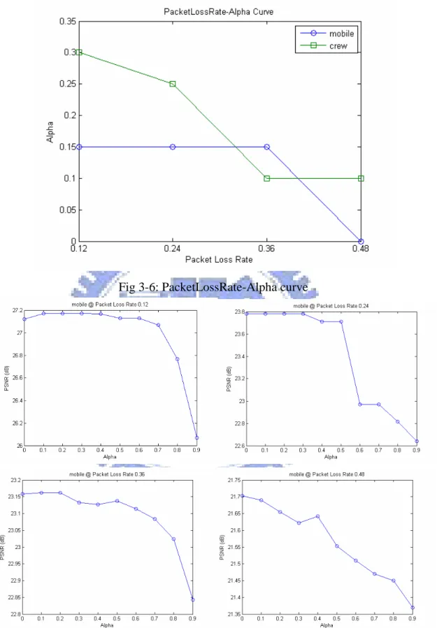
as the increasing of packet loss rate. From figure 3-7, we observe that there is a large range of α with which the associated PSNRs don’t differ much, for two videos with any packet loss rate. So we choose the α to be the median α values shown in figure 3-6 to be used in later

Fig 3-6: PacketLossRate-Alpha curve

Fig 3-7b: Alpha-PSNR curves of video “crew” under different packet loss rate

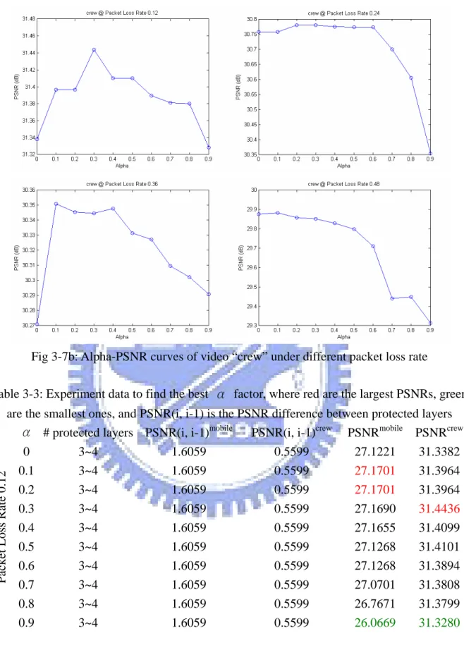
Table 3-3: Experiment data to find the best α factor, where red are the largest PSNRs, green are the smallest ones, and PSNR(i, i-1) is the PSNR difference between protected layers

α # protected layers PSNR(i, i-1)mobile

PSNR(i, i-1)crew PSNRmobile PSNRcrew

0 3~4 1.6059 0.5599 27.1221 31.3382 0.1 3~4 1.6059 0.5599 27.1701 31.3964 0.2 3~4 1.6059 0.5599 27.1701 31.3964 0.3 3~4 1.6059 0.5599 27.1690 31.4436 0.4 3~4 1.6059 0.5599 27.1655 31.4099 0.5 3~4 1.6059 0.5599 27.1268 31.4101 0.6 3~4 1.6059 0.5599 27.1268 31.3894 0.7 3~4 1.6059 0.5599 27.0701 31.3808 0.8 3~4 1.6059 0.5599 26.7671 31.3799

Packet Loss Rate 0.12

α # protected layers PSNR(i, i-1)mobile

PSNR(i, i-1)crew PSNRmobile PSNRcrew

0 2~3 6.1307 1.2494 23.7793 30.7573 0.1 2~3 6.1307 1.2494 23.7793 30.7577 0.2 2~3 6.1307 1.2494 23.7793 30.7802 0.3 2~3 6.1307 1.2494 23.7793 30.7802 0.4 2~3 6.1307 1.2494 23.7100 30.7748 0.5 2~3 6.1307 1.2494 23.7100 30.7736 0.6 2~3 6.1307 1.2494 22.9704 30.7736 0.7 2~3 6.1307 1.2494 22.9704 30.6994 0.8 2~3 6.1307 1.2494 22.8145 30.6041

Packet Loss Rate 0.24

0.9 2~3 6.1307 1.2494 22.6387 30.3538

α # protected layers PSNR(i, i-1)mobile

PSNR(i, i-1)crew PSNRmobile PSNRcrew

0 2~3 6.1307 1.2494 23.1585 30.2710 0.1 2~3 6.1307 1.2494 23.1615 30.3509 0.2 2~3 6.1307 1.2494 23.1615 30.3453 0.3 2~3 6.1307 1.2494 23.1330 30.3445 0.4 2~3 6.1307 1.2494 23.1265 30.3479 0.5 2~3 6.1307 1.2494 23.1376 30.3315 0.6 2~3 6.1307 1.2494 23.1139 30.3272 0.7 2~3 6.1307 1.2494 23.0831 30.3096 0.8 2~3 6.1307 1.2494 23.0235 30.3023

Packet Loss Rate 0.36

0.9 2~3 6.1307 1.2494 22.8426 30.2908

α # protected layers PSNR(i, i-1)mobile

PSNR(i, i-1)crew PSNRmobile PSNRcrew

0 1~2 0.4008 0.7484 21.7022 29.8771 0.1 1~2 0.4008 0.7484 21.6898 29.8818 0.2 1~2 0.4008 0.7484 21.6542 29.8577 0.3 1~2 0.4008 0.7484 21.6217 29.8512 0.4 1~2 0.4008 0.7484 21.6417 29.8297 0.5 1~2 0.4008 0.7484 21.5526 29.7990 0.6 1~2 0.4008 0.7484 21.5098 29.7108 0.7 1~2 0.4008 0.7484 21.4703 29.4410 0.8 1~2 0.4008 0.7484 21.4504 29.4487

Packet Loss Rate 0.48

0.9 1~2 0.4008 0.7484 21.3699 29.3134

3.3.3 Packetization

As mentioned in Section 3.3, when applying [5] to the extension of H.264/AVC, the

design of FFDO, since we estimate distortion of a GOP from the point of view of layers

instead of individual pictures, we have no need to enforce a packet to contain exactly one

picture layer data. In our implementation, every packet has the same length and it is possible

to have many NAL units in one packet or an NAL can be split into more than one packet. The

packet length of a FEC coding session which protects a layer of a GOP is the ceiling of video

data size/K, where K is from the protecting parameter (N, K) and is also the number of video

data packets.

Table 3-4 lists an example of protections determined by [5] and FFDO under the same

bandwidth and the same video bitstream. From the table and Fig. 3.4, it is easy to find out that

FFDO uses bandwidth much more efficiently than the proposed FEC selection algorithm in

[5], i.e., more bandwidth resource can be allocated to protection packets.

Table 3-4: Protection results determined by [5] and FFDO under same bandwidth (“0” denotes only the video data is sent and “x” denotes neither video nor protection data are sent.)

FFDO Algorithm in [5] GOP (Bandwdith) Layer: video size (Byte) Pkt Length (Byte) # of Protecting Packets Pkt Length (Byte) # of Protecting Packets 0: 12548 793 17 7948 4 1: 13419 847 14 5081 0 0 (75536) 2: 12570 794 14 8636 0 0: 12635 797 18 7932 1 1: 13599 858 10 5108 0 1 (49508) 2: 12650 x x 8511 0 0: 12026 759 17 7889 4 1: 13288 839 15 5194 0 2 (74748)

0: 12613 796 18 8182 1 1: 13042 824 10 5268 0 3 (48698) 2: 12419 x x 8691 0 0: 12806 808 17 8164 8 1: 14154 893 14 x x 4 (79258) 2: 13306 840 14 x x

3.4 Dynamic FEC-Distortion Optimization Algorithm

FFDO is based on the assumption that different frames in the same video layer exhibit

constant distortion. However, this is usually not the case for the real H.264 SVC videos. The

distortion (or PSNR) depends on the content of each video frame as well as the quantization

parameter used in each block. Due to the error propagation effect resulting from not only the

prediction coding across the video layers but also the temporal motion compensation coding

in each individual video layer, the distortion caused by different frame of a video layer can

also vary. As a result, the global optimal bit allocation of H.264 SVC and FEC shall be

calculated over all the possible bit allocation and packet loss combinations.

The main objective of our Dynamic FEC-Distortion Optimization (DFDO) algorithm is

to increase the decodable probability of important pictures when a layer of a GOP cannot be

completely received. After FFDO determines the best parameter configuration that indicates

the number of video layers to be protected and the protecting strengths, DFDO is applied to

each subscribed layer to reallocate the protecting packets. DFDO first classifies pictures into a

number of clusters which have different importance, and then reallocates the protecting

layer (or maximize the PSNR of whole layer).

3.4.1 Classifying Pictures to Clusters

Figure 3-8 is an example of picture classification, where pictures are classified by their

temporal level. As mentioned in Section 2.2, when hierarchical B prediction is applied, each

video layer can be decomposed to a number of temporal levels and every picture is predicted

by the reconstructed pictures of other two pictures of lower temporal levels. Therefore we can

say that the pictures belong to lower temporal levels are more important than those of higher

temporal levels.

In the implementation phase, a cluster may have unused spaces after all pictures of

cluster are filled inside. When this happens, we append the pictures of the next cluster to the

current one until there are no free spaces remained.

0 1 2 3 4 1 2 3 4 5 6 7 8 9 10 11 12 13 14 15 16 0 Pictures Clusters 0 1 2 3 4 1 2 3 4 5 6 7 8 9 10 11 12 13 14 15 16 0 Pictures Clusters

Fig. 3-8: An example of picture classification

3.4.2 Protecting Scheme

Figure 3-9 is an example of DFDO protecting scheme, blue parts are the clusters of video

data and green parts are the FEC data used to protect source clusters enclosed within brackets.

cluster (0,1,…,i). The summation of Mi must be the same as the number of packets allocated

to this layer by Flat FEC-Distortion Optimization algorithm. 0 1 2 3 4 (0,1,2,3,4) (0,1,2,3) (0,1,2) (0,1) (0) K₀ K₁ K₂ K₃ K₄ M₄ M₃ M₂ M₁ M₀ 0 1 2 3 4 (0,1,2,3,4) (0,1,2,3) (0,1,2) (0,1) (0) K₀ K₁ K₂ K₃ K₄ M₄ M₃ M₂ M₁ M₀

Fig 3-9: An example of DFDO protecting scheme

3.4.3 Algorithm

The main idea of Dynamic FEC-Distortion Optimization algorithm is to find the best

allocating patterns of protecting symbols such that the distortion of the whole video layer is

minimized (or the PSNR of the whole video layer is maximized), and can be illustrated as

equation (12). An allocating pattern is a vector where each element determines the number of

protecting symbols for corresponding cluster. M* is the set of all possible patterns. PSNR*(s,p)

is the corresponding PSNR when applying allocating pattern s to a video layer with average

packet loss rate p. The PSNR of whole video layer can be estimated as the summation of

PSNR contributed by each cluster and is illustrated as equation (13), where p*i means the

decodable probability of the only first i clusters and D*i is the corresponding PSNR

(s,p)

S

"

arg

max

PSNR

*

=

₍₁₂₎

∑

⋅

=

D

p

(s,p)

PSNR

*

(13)

Figure 3-10 is a binary tree for 3-layer video. Each path which starts from root and ends

at leaf forms a decoding path. A Y-edge denotes that the corresponding source cluster is

decodable, and an N-edge means that the corresponding source cluster is undecodable. For

example, Path 0Y1N2Y denotes the event that cluster 0 is decodable followed by cluster 1,

which is undecodable, and further followed by decodable cluster 2. Since cluster (0,1,…,i)

protects source clusters 0 to i at the same time, all source clusters can be decoded at the end of

the path 0Y1N2Y.

The decodable probability of the only first i clusters, p*i, can be derived by such binary

trees. In figure 3-10, p*3 is the sum of the probability of decoding paths 0Y1Y2Y, 0Y1N2Y,

0N1Y2Y, and 0N1N2Y. And for p*2, its value is the sum of the probability of decoding paths

Fig 3-10: A binary tree for 3-layer video

We summarize p*i in equation forms, as illustrated in (14) to (17). Equation (15)

corresponds to the decodable probability of paths which start from ID-Y and there are pvK

packets received from source clusters 0 to ID-1. Equation (16) corresponds to the

undecodable probability of paths which start from ID-N and there are pvK packets received

from source clusters 0 to ID-1. Equation (17) calculates the minimal number of packets

required to decode source clusters 0 to ID. C is the number of source clusters in layer, p is the

average lost rate, Ki is the number of source symbols in cluster i and Mi is the number of

protecting symbols of protecting cluster (0,1,…,i).

)

0

,

,

0

(

)

0

,

,

0

(

i

N

i

Y

p

=

+

₍₁₄₎

( )

(

)

( )

(

)

⎪

⎪

⎩

⎪

⎪

⎨

⎧

⎥

⎦

⎤

⎢

⎣

⎡

+

+

+

×

−

≥

=

_∑

_∑

otherwise

ID

K

t

ID

N

ID

K

t

ID

Y

p

p

C

C

t

ID

if

pvK

t

ID

Y

,

,

,

1

,

,

1

)

1

(

,

0

)

,

,

(

(15)

(

)

(

)

⎪

⎪

⎩

⎪

⎪

⎨

⎧

⎥

⎦

⎤

⎢

⎣

⎡

+

+

+

+

+

×

−

−

=

=

_∑

_∑

otherwise

i

pvK

t

ID

N

i

pvK

t

ID

Y

p

p

C

C

t

ID

if

pvK

t

ID

N

,

,

,

1

,

,

1

)

1

(

1

,

0

)

,

,

(

(16)

∑

=

K

ID

K

)

(

(17)

The distortion measuring function D*i, which is corresponded to p*i, can be estimated as

equation (18), where PSNRj is the summation of PSNR contributed by pictures in cluster j.

The β is a leaky factor to reflect the quality degradation caused by reference to an

unavailable and error concealed picture. The exponential form of β is due to the

hierarchical B prediction.

1

0

,

=

∑

+

∑

×

≤

<

β

β

PSNR

PSNR

D

₍₁₈₎

3.4.4 How to determine β factor

The value of β is chosen experimentally. We protect the video sequences “ice” and

“city” with α 0.15 and different βs and select the best one which shows the highest PSNR.

Each protected stream passes 100 lossy channels which have the same packet loss rate

simulation results of sequence “ice” and “city”, respectively. From figures 3-11a and 3-11b, we can observe that DFDO has stable and best performance when β is between 0.6 to 0.95.

Thus, we choose 0.75 in further simulations.

Table 3-5: Encoding parameters and PSNRs

Layer ID Resolution Bit-rate (kbit/sec) PSNRice (dB) PSNRcity (dB)

0 QCIF 200 30.1402 25.0721

1 QCIF 400 30.5005 25.2716

2 CIF 600 32.2488 26.7457

3 CIF 800 32.6895 27.2123

4 4CIF 1000 36.3041 30.9114

IV. Simulation Results

4.1 Simulations for Flat FEC-Distortion Optimization

4.1.1 Environment

We prepare two 300-frame video sequences, mobile and crew, which are encoded with

the same parameters listed in table 4-1. For each video sequence, we simulate with four

packet loss rates which are 0.12, 0.24, 0.36 and 0.48. The packet lost patterns are generated

with independent and identical distribution. The bandwidth is given as shown in figure 4-1, where for odd-ID GOPs we give more bandwidth and for even ones we give less. Theα

factor used in FFDO is 0.15, as described in Section 3.3.2. Every simulation value is averaged

from 100 times of simulations with different loss patterns. The protection result for both

videos with four packet loss rates are listed in table 4-2, and the graphs of simulation results

are illustrated in figure 4-2 and 4-3.

Table 4-1: Encoding parameters and PSNRs

Layer ID Resolution Bit-rate (kbit/sec) PSNRmobile PSNRcrew

0 QCIF 200 21.5101 29.5959

1 QCIF 400 21.9109 30.3443

2 CIF 600 28.0416 31.5937

3 CIF 800 29.6475 32.1536

Fig 4-1: Given bandwidth

4.1.2 Simulation Results

Table 4-2: Protection results (The number is the amount of protecting symbols)

mobile crew

Packet loss rate Packet loss rate

GOP Layer 0.12 0.24 0.36 0.48 0.12 0.24 0.36 0.48 0 8 16 18 28 6 14 23 29 1 7 15 14 17 4 10 17 19 2 7 14 13 0 4 10 17 10 3 6 X X X 3 5 X X 1 4 X X X X 2 X X X 0 5 17 21 46 8 13 24 38 1 4 11 7 X 5 6 14 0 2 2 3 X X X 5 0 X X 0 10 16 18 28 11 21 23 30 1 7 15 14 18 9 18 19 17 2 7 15 14 0 8 17 15 11 3 3 5 X X X 7 X X X 0 5 17 21 45 7 18 21 47 1 4 11 7 X 4 13 10 X 4 2 3 X X X 3 X X X 0 8 16 18 29 10 19 21 32 1 7 15 14 17 8 16 16 21 2 7 14 13 0 7 16 14 0 5 3 6 X X X 6 X X X 0 6 16 22 46 7 17 20 45 1 3 11 6 X 3 12 9 X 6 2 3 X X X 2 X X X

0 8 16 18 28 9 16 20 35 1 7 15 14 17 6 13 12 24 2 7 14 13 0 6 12 9 X 7 3 6 X X X 4 X X X 0 5 16 21 46 6 18 21 46 1 4 11 6 X 3 13 10 X 8 2 3 X X X 2 X X X 0 9 17 18 28 9 18 20 38 1 7 15 14 17 6 14 13 28 2 7 14 14 0 6 12 11 X 9 3 6 X X X 5 X X X 0 5 16 21 44 14 15 21 38 1 3 10 5 X 12 11 4 X 10 2 3 X X X X X X X 0 8 16 17 28 8 16 20 34 1 7 14 14 15 6 13 12 22 2 7 14 13 0 6 12 9 X 11 3 6 X X X 5 X X X 0 5 16 21 41 7 14 23 38 1 4 11 6 X 3 9 0 X 12 2 3 X X X 1 X X X 0 8 16 17 28 8 16 22 31 1 7 14 13 14 6 12 14 18 2 7 13 13 0 6 11 0 X 13 3 6 X X X 4 X X X 0 5 16 20 41 13 15 23 38 1 3 10 6 X 11 9 0 X 14 2 3 X X X X X X X 0 8 16 17 28 8 16 20 32 1 7 14 13 15 6 13 12 20 2 7 13 13 0 6 12 8 X 15 3 6 X X X 5 X X X 0 5 16 22 41 7 16 20 41 1 4 11 4 X 3 10 6 X 16 2 3 X X X 1 X X X

0 8 15 17 28 9 17 20 34 1 7 14 13 13 6 14 13 25 2 7 13 12 0 6 13 10 X 17 3 5 X X X 5 X X X 0 5 16 22 40 7 15 24 39 1 4 11 4 X 3 10 0 X 18 2 3 X X X 0 X X X 0 9 17 19 32 7 14 22 39 1 7 15 16 27 5 10 17 29 2 7 15 16 26 4 9 15 X 3 6 11 8 X 3 5 X X 19 4 4 X X X 3 X X X

Fig 4-3: Simulation results of sequence crew with different packet loss rates

4.2 Simulations for Dynamic FEC-Distortion Optimization

4.2.1 Environment

We first encode two sequences, “football” and “soccer”, both have frame rate 30 fps, to

compare the protection performance between FFDO and DFDO. The encoding parameters are listed in table 4-3. The packet loss rate is 0.285714; the α factor used in FFDO is 0.15, and

the β factor used in DFDO is 0.75. The bandwidth distributions for two videos are given in

Fig 4-4a: Given bandwidth for football @ 30 fps

Fig 4-4b: Given bandwidth for soccer @ 30 fps

Table 4-3: Encoding parameters and PSNR for sequences football and soccer at 30fps

Layer ID Resolution Bit-rate (kbit/sec) PSNRfootball (dB) PSNRsoccer (dB)

0 QCIF 200 27.5387 28.3235

1 QCIF 400 28.9634 28.9213

2 CIF 600 31.0809 30.0142

3 CIF 800 32.1219 30.4611

4 4CIF 1000 32.3232 32.1135

Figures 4-6a and 4-6b are the simulation results of football with FFDO and DFDO,

respectively. For the convenience of comparison, we also present the graph of the PSNR

difference between DFDO and FFDO, as shown in 4-6c, where the positive area indicates that

DFDO outperforms FFDO by 0.4 dB in average. In fig 4-6d, we compare both algorithms

with sequence soccer, and it shows that DFDO outperforms FFDO by 0.7 dB, averagely.

From figure 4-6c, we can observe that DFDO outperforms FFDO even more when a

observed from the protection result as shown in table 4-5.

Further, in order to examine the performance of DFDO when the video content has wide

and global motion, we down-sample the sequences football and soccer from 30fps to 15fps.

The encoding parameters are listed in table 4-4, such as packet loss rate and both leaky factors

used in simulation remain the same. The graph of given bandwidth is shown in figure 4-5. The

simulation results for both videos are shown in figure 4-7a and 4-7b, and DFDO outperforms

FFDO by 0.5~0.7 dB. In the case of football, it is almost twice as compared with the 30fps

version.

Fig 4-5a: Given bandwidth for football @ 15 fps

Table 4-4: Encoding parameters and PSNR for sequences football and soccer at 30fps

Layer ID Resolution Bit-rate (kbit/sec) PSNRfootball (dB) PSNRsoccer (dB)

0 QCIF 200 28.4286 28.6826

1 QCIF 400 29.9313 29.1768

2 CIF 600 32.7111 30.3753

3 CIF 800 34.2528 30.8541

4 4CIF 1000 34.4149 32.9559

We also compare both algorithms under the case of misestimate of packet loss rate.

Figure 4-8 shows the simulation results on the 30fps and 15fps football sequences, where the

x axis means the actual packet loss rate in channel and the y axis means how much DFDO

outperforms FFDO. The misestimated packet loss rate is 0.285714. And we can observe that,

although the packet loss rate is not estimated accurately, our DFDO algorithm still

4.2.2 Simulation Results

Table 4-5: Protection results (The number is the amount of protecting symbols) DFDO

GOP Layer FFDO

M0 M1 M2 M3 M4 0 18 0 0 0 0 18 1 16 0 0 0 0 16 2 15 0 0 0 0 15 3 13 0 0 0 0 13 1 4 9 0 0 0 0 9 0 15 0 0 0 0 15 1 11 0 0 0 0 11 2 10 0 0 0 0 10 2 3 6 0 0 0 6 0 0 14 0 0 0 0 14 1 8 0 0 0 7 1 3 2 4 0 0 4 0 0 0 14 0 0 0 0 14 4 1 4 0 0 4 0 0 5 0 4 0 0 4 0 0 0 14 0 0 0 0 14 6 1 4 0 0 4 0 0 0 15 0 0 0 0 15 1 8 0 0 0 8 0 7 2 6 0 0 0 6 0 0 16 0 0 0 0 16 1 12 0 0 0 0 12 2 11 0 0 0 0 11 8 3 4 0 0 4 0 0 0 18 0 0 0 0 18 1 15 0 0 0 0 15 2 14 0 0 0 0 14 3 11 0 0 0 0 11 9 4 6 0 0 0 6 0

0 15 0 0 0 0 15 1 12 0 0 0 0 12 2 10 0 0 0 0 10 10 3 5 0 0 0 5 0 0 14 0 0 0 0 14 1 8 0 0 0 7 1 11 2 5 0 0 0 5 0 0 14 0 0 0 0 14 12 1 4 0 0 4 0 0 13 0 4 0 0 4 0 0 0 14 0 0 0 0 14 14 1 4 0 0 4 0 0 0 13 0 0 0 0 13 1 9 0 0 0 0 9 15 2 4 0 0 4 0 0 0 15 0 0 0 0 15 1 11 0 0 0 0 11 2 11 0 0 0 0 11 16 3 5 0 0 0 5 0 0 18 0 18 X X X 1 16 0 16 X X X 2 15 0 15 X X X 3 12 0 12 X X X 17 4 5 5 0 X X X

Fig 4-6a: Simulation result of FFDO with football, average PSNR is 28.4065 dB

Fig 4-6c: The difference of simulation results between DFDO and FFDO, football @ 30 fps

Fig 4-7a: Simulation result between DFDO and FFDO, football @ 15 fps

Fig 4-8: Simulation result with different packet loss rate, sequence football

Fig 4-9a: mobile Fig 4-9b: crew Fig 4-9c: harbour

V. Conclusion

In multimedia transmission, forward error correction code is a useful technique to avoid the retransmission of lost packet, which may lead to a large delay and is not feasible to real-time play. The erasure code protects data by adding some redundancies to the source information. And for a video stream transmitted over a lossy channel which has limited bandwidth, it is important to distribute bandwidth among video data and protection data efficiently in order to have good visual experience.

In this paper, we first modify [5] to be flat FEC-distortion optimization (FFDO) algorithm, which not only can adapt to the scalable video streams encoded with H.264/MPEG-4 AVC scalable extension standard but also can take account inter-layer prediction. Then we propose the dynamic FEC-distortion optimization (DFDO) algorithm, which further improves FFDO so that the pictures within the same video layer of a GOP are protected according to their importance. Thus, when a video layer of GOP can not be completely received, DFDO has more chance to recover important pictures than FFDO does.

The simulation results show that the average PSNR of DFDO outperforms FFDO about 0.4 dB. If we make the video content moves wider by down-sampling from 30fps to 15 fps,

DFDO outperforms FFDO about 0.8 dB. We also navigate the performance of DFDO under

the case of misestimate of packet loss rate, and the simulation results show that DFDO still outperforms FFDO. Thus we can conclude that protecting pictures within the same video layer according to their importance can improve the visual quality.

Reference

[1] ETSI, “Digital Video Broadcasting (DVB): Transmission systems for handheld terminals,” ETSI standard, EN 302 304 V1.1.1, 2004.

[2] J. Byers, M. Luby, and M. Mitzenmacher, “A Digital Fountain Approach to Asynchronous Reliable Multicast,” IEEE Journal on Selected Areas in Communications, 20(8), pp. 1528-1540, October 2002.

[3] M. Luby et al., “Raptor Codes for Reliable Download Delivery in Wireless Broadcast Systems,” IEEE CCNC, Las Vegas, NV, Jan. 2006.

[4] 3GPP TS 26.346 V6.4.0, “Technical Specification Group Services and System Aspects; Multimedia Broadcast/Multicast Service (MBMS); Protocols and Codecs,” Mar. 2006. [5] W.-T. Tan, A. Zakhor, “Video multicast using layered FEC and scalable compression,”

IEEE Transactions on Circuits and Systems for Video Technology, March 2001.

[6] H.-F. Hsiao, A. Chindapol, J. A. Ritcey, and J.-N. Hwang, “Adaptive FEC Scheme for Layered Multimedia Streaming over Wired/Wireless Channels,” Workshop on Multimedia Signal Processing, IEEE, pp. 1-4, Oct. 2005.

[7] S.-R. Kang and D. Loguinov, “Modeling Best-Effort and FEC Streaming of Scalable Video in Lossy Network Channels,” IEEE/ACM Trans. on Networking, Feb. 2007. [8] W.-T, A. Zakhor, “Real-Time Internet Video Using Error Resilient Scalable Compression

and TCP-Friendly Transport Protocol,” IEEE Transactions On Multimedia, Vol. 1, No. 2, JUNE 1999

[9] H. Schwarz, D. Marpe, and T. Wiegand, “Overview of the Scalable H.264/MPEG4-AVC Extension,” International Conference on Image Processing, IEEE, Oct., 2006.

[11] ITU-T Rec. & ISO/IEC 14496-10 AVC, “Advanced Video Coding for Generic Audiovisual Services,” version 3, 2005.

[12] San Ling and Chaoling Xing, “Coding Theory, A First Course”, Cambridge University Press

[13] http://ip.hhi.de/imagecom_G1/savce/index.htm

[14] Yao Wang, Jorn Ostermann, and Ya-Qin Zhang, “Video Processing And Communications”, Prentice Hall, pp. 349

[15] S. R. Hankerson, D. G. Hoffman, D. A. Leonard, C. C. Lindner, K. T. Phelps, C. A.

Rodger, J. R. Wall, “Coding Theory And Cryptography, The Essentials, 2nd edition”,

Marcel Dekker, Inc.

[16] Jerome Lecan and Jerome Fimes, “Systematic MDS Erasure Codes Based on Vandermonde Matrices”, IEEE Communications Letters, Vol. 8, No. 9, Sep. 2004

[17] I.Gohberg and V.Olshevsky, “Fast algorithms with preprocessing for matrix-vector multiplication problems”, Journal of Complexity, 1994