Data classification with a relaxed model of variable kernel density estimation

Data Classification with

a Relaxed

Model of

Variable

Kernel Density

Estimation

Yen-JenOyang*, Yu-Yen Ou, Shien-Ching Hwang,

Chien-Yu Chenl,andDarbyTien-HauChang

Department of Computer Science and Information Engineering, National Taiwan University, Taipei, Taiwan, R.O.C.

'Graduate Schoolof BiotechnologyandBioinformatics, Yuan-ZeUniversity, Chung-Li, 320, Taiwan, R.O.C.

yjoyang@csie.ntu.edu.tw; yien@csie.ntu.edu.tw; schwang@mars.csie.ntu.edu.tw

Abstract

In recent years,kerneldensity estimationhas beenexploited by

computer scientists to model several important problems in

machine learning, bioinformatics, andcomputervision.

How-ever,incasethedimension of the datasetishigh, then the

con-ventional kernel density estimators suffer poor convergence

rates ofthe pointwisemean square error(MSE)and the inte-grated mean square error (IMSE). Therefore, design of a

novel kernel density estimatorthat overcomesthisproblem has been agreatchallenge formany years. Thispaperproposesa

relaxed model of the variable kernel density estimation and analyzes its performance in data classificationapplications. It is proved in this paper that, in terms ofpointwise MSE, the convergence rateof therelaxed variablekerneldensity

estima-tor canapproachO(n'l)regardless ofthedimensionofthe data

set,where nis the number ofsamplinginstances. Experiments with the data classification applications have shown that the improved convergence rate of the pointwise MSE leads to

higher prediction accuracy. Infact, the experimental results have alsoshown that the data classifier constructed based on

therelaxed variable kerneldensityestimator iscapable of de-livering thesamelevelofprediction accuracy as theSVMwith theGaussian kernel.

Keyterms: kernel density estimation, variable kernel

den-sity estimation, radial basis function, RBF network, data classification.

I.INTRODUCTION

Kernel density estimation isaproblemthat has been studied

by statisticians for several decades [1, 5, 10, 22, 23]. In recentyears,kerneldensityestimationhas beenexploited by

computer scientists tomodel several importantproblems in machine learning [9], bioinformatics [6], and computer vi-sion [3]. The problem definition ofkernel density estima-tion is as follows: given a set ofsampling instances {s1,

S2, ..-,

sn

randomlytaken from the targetprobability distri-bution with an unknown form in an m-dimensional vector

space, we want to construct an estimator of the following

formthatprovides a good approximation of the target

prob-ability densityfunction:

(I)

n

f(v)= w,

b(v;s,,cr,)

,where

1=1

1)visa vectorin them-dimensionalvectorspace; 2)w, and aiaretheweightandwidth ofthe i-th kernel

function, respectively.

So far, manytypesofkernel functions have beenproposed forkerneldensityestimation. If the popular Gaussian func-tion isemployed, then theformofequation (1)becomes

f(v)

=

Zw,

exp{-

li2

5,

I2)J

(2)

wherelIv-

silI

is thedistance between vectorsvand si.

Thereareseveral types ofkerneldensityestimators

pro-posed bystatisticians[22]. Thebasiconeis thefixed kernel

density estimator, which is of the following form with the

Gaussian functionemployed:

J(v I I

nex

( V- S 112'

f(v)

=

n.

42

)exj1p-

' I (3)

Since inafixed kerneldensityestimator allkernelfunctions have the same width, it is ofinterest to investigate the ef-fectsofthegeneralizedmodels.

Onemajor approach thathas been proposedto

general-ize the fixedkernel density estimator is the variable kernel density estimator[5]. Thegeneralform of the variable ker-nel density estimator with the Gaussian function is as fol-lows:

f(v)

=- -1 exp' II Sj

(4)

ff)n

=,

(6e(Si)t

2(OR,(s)r

where 9is the so-called smoothing parameter and

Rk(si)

is the distance between samplinginstancesiand its k-th near-estneighbor. As equation (4) shows, in a variable kernel

*Towhomcorrespondence should be addressed.

density estimator, the width of each kernel function is a

function ofthe local density surrounding the sampling in-stance. The motivation behind thedevelopment of the vari-ablekerneldensity estimator istoexploit the local distribu-tionsurrounding eachsampling instance. Inthisregard,the adaptive kernel density estimator represents another major

alternative approach to generalize the fixed kernel density

estimator[1, 22].

The main problem with the conventional kernel density

estimators inhandling highdimensional datasetsis that the convergence rate of thepointwise MSE(mean square error) turns poor as the dimension increases. For example, with the Gaussian function, the convergence rate ofthe fixed kernel density estimator is

0(nf4/(m+4)),

where m is the di-mension of the data set [22]. With some specific types of kernel functions, the convergence rate can be slightly im-proved to

0(n-'

/(m+8))

. Nevertheless,regardlessof the type

of the kemel functions employed, the pointwise MSE ofa

conventional kernel density estimator converges at an

ex-tremely slow rate in case the dimension of the data set is high.

One important development in recent years toward the

design of a multivariate kernel density estimator that fea-turesahigherconvergence rateofthepointwiseMSEis due toSain and Scott [21]. Inthearticle,Sain and Scott showed that it is feasible to make the

pointwise

MSE ofthe

so-called locally adaptive kerneldensity estimator converge at

O(n-')

inregionswhere the target

probability

density

func-tion is convex. Nevertheless, their theorems hold only in

suchregions.

This paper proposes a relaxed model of the variable ker-nel density estimation. The most important mathematical propertyofthe relaxed model is that the convergencerateof the pointwise MSE can approach

0(n-'), regardless

of the dimension of the data set. In fact,the development ofthe relaxed variable kernel density estimation stems from our

recent work with the RBF(radial basis function) network [18, 19]. The experimental results reported in our recent article [19] show that the proposed learning algorithm for the RBF network, which is based on a preliminary version of the relaxed variable kemel density estimator, is capable

of delivering the same level of accuracy as the

SVM(supportvector machine) [7, 11] in data classification

applications. On the otherhand, itgenerally takes far less time than the SVMalgorithm for constructingadata classi-fier with anoptimized parameter setting, due to its average timecomplexity ofO(n logn). Therefore, it isofinterest to investigate the properties of the relaxed model of variable

kerneldensity estimation from a theoretical aspect.

Inthemathematicalanalysis presented in this paper, the discussion will focus on how the pointwise MSE of akernel density estimator behaves, because the application ad-dressed in this paper is data classification. With respect to data classification accuracy, the main concern is the

point-wise MSE in the critical region, instead of the IMSE(integrated MSE) [22] over the entire distribution.

In the following part of this paper, section II discusses the works related to thestudy presented in this paper. Sec-tion III elaborates the mathematical properties of the relaxed variable kernel density estimator. Section IV reports the experiments conducted to evaluate its performance in data classification applications anddiscusses interesting observa-tions. Finally, concluding remarks are presented in section V.

II.RELATED WORKS

The general form of a kernel density estimator shown in equation(1) is in fact the same as that of an output node of an RBFnetwork. In the machine learningresearch commu-nity, there have been quite a few learning algorithms pro-posed for RBF networks. The learning algorithm deter-mines the number of nodes in the hidden layer, the activa-tion functions associated with the hidden nodes, and the weights associated with the links between the hidden and outputlayers.

Basically, there are two categories of algorithms

pro-posed for constructing RBF networks

[2,

16]. The first

category ofalgorithms simply places one radial basis

func-tion at each sampling instance [17] and yields the same

mathematical form for each output node as equation (1). The kernel density estimationbasedalgorithms proposedin recentyears represent thelatest developments in the design of thiscategory ofalgorithms [8, 9]. Onedesirable feature ofthe kernel density estimation based approach is its low timecomplexity ofO(nlogn)forconstruction of a classifier. However, because the RBF network constructed with this categoryofalgorithmsisinstancebased,datareduction may need to be invoked to reduce the size of the RBF network constructed. Anotherproblemwith this approach is that the

conventional kernel density estimation algorithms can not deliver satisfactory accuracy in handling high dimensional data sets. Inthisregard,ourrecentstudieshave shown that theRBFnetwork constructed with the earlier version of the relaxed model of variablekernel densityestimation is capa-ble ofdeliveringthe same level of accuracy as the SVM in data classificationapplications[18, 19].

The second category ofalgorithms proposed for

con-structing RBF networks resorts to a regularization process tofigureouttheoptimal parametersettings of the RBF net-work [12, 13, 14, 15]. Because the regularization process involves computing the inverse of a matrix with dimension equal to the number of hidden nodes in the network, it is

typical that a clustering analysis on the training data set is conducted to deternine where the radial basis functions

should be located [2, 12, 14]. Oneof the main advantages of this approach is that the size of the RBF network

con-structed is relatively small. A comprehensive analysis on thecharacteristics of the RBF network constructed with this categoryof algorithmscanbefoundin oneof our latest arti-cles [20].

Insummary,kerneldensity estimation and regularization represent two most recent approaches proposed for con-struction of RBF networks. Both approaches offer some advantages and suffer some deficiencies. Nevertheless, the

experimental resultspresented inthis article and in another

our latest article show that with the state-of-art algorithms

both approaches can deliver the same level of accuracy in data classification applications [20]. Therefore, it is really

up to the user to select the approach that is most suitable based on the characteristics ofthe datasetbeinghandled.

III. THERELAXEDMODELOFVARIABLE KERNELDENSITY ESTIMATION

Let {SI, s2, ...,

s,}

bea setofsamplinginstances

independ-ently andrandomlytakenfromadistribution with

probabil-itydensity functionfinanm-dimensionalvectorspace. The

generalform of the relaxed variablekerneldensityestimator is asfollows:

f(v)

=-* E (E/ O )= e

2a

)a

where

1) a,

=fi_[nf(si)]-1a;

2) aisapositiverealnumber;

3)1 is thesmoothingparameter;

4)

f(s,

) isapilotestimate of

f(si).

In our implementation, the nearestneighbor estimator [19,

22] shown in the following has been

adopted

to obtain a

pilotestimate of

f(si):

(k +1) [(Rk si

)f,)rnm

f(Si)

[ ('l J

~f(si),

(6)

n

r(m

+)

1(6

where

Rk(s,)

is thedistance betweensamplinginstancesiand itsk-thnearestneighbor.

In the following discussion, without loss of

generality,

wecanassumethat itis thepointwiseMSE attheoriginthat is ofour concern. In addition, we will set the

smoothing

parameter

,J

asfollows:

h

pl

= {fa(h+l) ) with h>> aand h>>m.

Withsuchsetting,wehave Ia - 0 as n

-+oo.

Thefirsttheoremthat wewill proveisthat, with proper

setting of

parameter

a, we can make the relaxed variable

kernel density estimator shown in equation (5) unbiased, providedthatnissufficiently large.

Theorem 1. Let f(v) be a relaxed variable kernel density estimator

of1(v)

as shown in equation (5). Then, when n is sufficiently large, there exists a real number a'

within (m-

1,rm

+1) that makes E[f(O)]=f(O), provided that 0

<A0)

<

a0.

Proof.

A

complete

proof

is

presented

in

Appendix

A. O

InTheorem 2, we will derive a closed form of the

vari-anceofthe relaxed variable kernel density estimator. Theorem 2. Let f(v) be arelaxed variable kernel density

estimator

ofJAv).

Then, whennis sufficiently large, Var[f(O)]~T

f(O)(O)

Var[fO)]

=(2,1.)a

nmlrna-I/J2arn

Proof.

Acompleteproof is presented in Appendix B. LI Theorem 3. Assume that the smoothing parameter 8 in equation (5) is set to O(n

(hta(4+l)))

with h>> aand h>> m.

Then, whennis

sufficiently

large, there exists a real number

a within (m-1,m+1) that makes

MSE[f(O)]_O(n-I+7),

where 7-0 as

h-+0o.

Proof.

Bydefinition,

MSE[f(O)]

=

VAR[f(O)]

+[E[f(O)]-

f(0)]2.

AccordingtoTheorems 1 and2, whennissufficiently large,

we canfmdan LX within (m-l,m+

1)

that makes

MSE[f(O)]=

{VAR[f(O)]

+

[E[f(O)]

_

f(O)2

}

0 n)(h)=0 O(n 1+17)

where q-0 as h-o+0. E]

So far, we have shown that we can make the conver-gence rate ofthe pointwise MSE of the relaxed variable

kernel densityestimator presentedin equation (5) approach

0(n-'),

regardlessof the dimension of thedataset, provided

thatn issufficiently large. However, incase nisnot

large

enough, then

aA

in Theorems I and 3 may fall in a wider rangebeyond (m -1,m+1).

IV.IMPLEMENTATIONANDEXPERIMENTAL RESULTS This section addresses the implementation ofa supervised

learning

algorithm basedonthe relaxedvariablekernel

den-sity estimator presented in Section III and reports the

ex-periments conducted to evaluate its

performance.

It is as-sumed that the

sampling

instances in the data set are distrib-uted in an m-dimensional vectorspace. The

learning

algo-rithm will construct one kernel density estimator based on

oneclass ofsamplinginstances in the vector space. Then, a queryinstance locatedat vispredictedtobelongtotheclass

that gives the maximum value of the likelihood functions defined in thefollowing:

Lij(v)

= I

fI(v)

where

Sj

is the set of

class-j

training instances,Sis the set of training instances of all classes, and

fj

(v) is the kernel

density estimator of

class-j

training instances. In our im-plementation, wehave observed that R(s,) inequation (6) is determined by one single training instance and therefore could beunreliable,ifthe data set isnoisy. Accordingly,we

have adopted

R(si)

definedinthefollowingtoreplace

R(si)

inequation (6):

m

(k

h=I

where

s1, '2,

...,

sk

arethe k nearesttraininginstances of the same class as

si.

The basis of employing

R(si)

can be found in [19]. Asfar as the timecomplexityof thelearning algorithm is concerned, it has been shown in

[19]

that the average time complexity for constructing a data classifier based on the relaxed variable kernel density estimator is boundedby O(n log n), wheren is total numberoftraining

instances. Furthermore, the average time complexity for predicting the classes of n' query instances is bounded by O(n'log n).

Intheremainingpart ofthis section, we will reports the

experiments conducted to evaluate the performance of the data classifier constructed based on the relaxed variable kernel density estimator. In the experiments, we have

em-ployed both synthesized datasets and some ofbenchmark datasets in the UCIrepository [4].Theexperimentswith the

synthesized datasets have been designed to pin down the maincharacteristics of the data classifier. On the otherhand,

theexperiments with the UCI benchmark datasetsareaimed atstudyinghow the data classifierperformsinhandlingreal data sets.

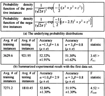
TABLE

1(a)

shows the underlying probability distribu-tions of the synthesized datasets, from which the training

andtestinginstances arerandomlytaken with the total num-ber ofnegative instances equalto20times the total number of positive instances. The design of the synthesized data

sets is aimed at emulating skewed data sets with very few

positive instances. Intheexperiments,wefocusonthe

dis-tributionsofinstances intheproximity of the origin. Inthis region, the number of positive instances is slightly larger than the number ofnegative instances. In our study, we have investigated the effects of replace m in equations (6) and(7)by a, which

implies

that we havetreated the data set as ifit were in an a-dimensional vector space. Since the resultshave shown that replacing m by a generally leadeds

tohigher classification accuracy, in the following discussion we will only report the experimental results obtained with thispractice adopted.

TABLE 1(b)and TABLE 1(c)show the summarized re-sults with 20 independent runs of the sameexperiment pro-cedure. For each run of theexperimentreported in TABLE l(b), a total of 10,000,000 training instainces along with 2,500,000 testing instances have beenindependently gener-ated and only the instances that fall within 0.2 away from theorigin have been included in the data set. For each run of the experiment reported in TABLE l(c), a total of 20,000,000 training instances along with 5,000,000 testing instances have been independently generated and only the instances that fall within the same sphere have been in-cluded in the data set. Then, the relaxed variable kernel density estimator based data classifiers constructed with the

training instances under various parameter settings have been used to predict the classes of the testinginstances. In these experiments,parameter k in equations (6) and (7) has been set to 30 and themaximum prediction accuracies ob-tained with the following possible combinations of a and ,B havebeenreportedin TABLE1(b)and TABLE1(c):

{a la=1.0,l1.1,1.2,...,4.0}x

{/61,6

=0.5, 0.6, 0.7,..., 6.0} . Since the underlying probability distributions are in a 3-dimensional vector space, whenais set to3,equation (5)in fact becomes the conventional variable kernel density esti-mator. Accordingtothe results summarized in TABLE 1(b)

and TABLE 1(c), the confidence levels for accepting that thedata classifier based on the relaxed variable kernel

den-sity estimatoris capable ofdelivering higher prediction ac-curacy than the data classifier based on the conventional variable kernel density estimator are over 90% and 95%,

respectively.

TABLE 1. EXPERIMENTALRESULTSWITH THESYNTHESIZEDDATASETS.

Probability density 1 (X2 2 2)

function of the posi- ex x y ))

tive instances

functionof the nega- (,23exp +z

tiveinstances 2

(a)Theunderlying probability distributions Avg.#of Avg. #of Accuracy Accuracy F

training testing a=1.3,/3=1.6 a=3,/=0.8 statistic

instances instances ( ±a) (')u a)

3629.6 921.95 52.32% 51.30% 3.45>

±1.91%

±1.62% F,,1

(b) Summarized experimentalresultwith the first data set. Avg. #of Avg.#of Accuracy Accuracy F

training testing a=1.0,fl=2.9 a=3,/i=0.8 statistic

instances instances (u±a) ±uia)

7271.2 1810.45 52.84% 51.97% 4.52>

±1.300/o ±1.30/ F0.05

TABLE2. COMPARISONOF THE PREDICTION ACCURACY OF ALTERNATIVE APPROACHES WITH SEVENBENCHMARK DATASETSINTHE UCI REPOSITORY[4]

iris wine Vowel segment satimage letter shuttle Average |

Relaxed variable KDE 96.67 99.44 99.62 97.403 92.45 97.12 99.94 97.52

Parameter a in

equation

(5) 4 1 1 1.4 2.1 2 3

-Conventional variableKDE 96.67 95.52 99.62 97.27 89.35 96.68 99.94 96.44

Dimension of the data set 4 13 10 19 36 16 9

-SVM(Guassian kernel) 97.33 99.44 99.05 97.40 91.30 97.98 99.92 97.49

SVM(Linearkernel) 97.33 98.88 81.82 95.80

1

85.85 85.14 98.10 91.85

TABLE 2 shows how the dataclassifier based on the re-laxedvariable kernel density estimator performs, in terms of prediction accuracy, in comparison with the alternative ap-proaches with 7 benchmark data sets from the UCI reposi-tory. The experimental procedure employed in this experi-mentis exactly the same as that employed in our recent arti-cle[19].Inaddition, the implementation of the relaxed vari-able kernel density estimator based classifier is essentially the same as theimplementation detailed in our recent article

[19]. The only difference between these two

implementa-tions is that ainequation (5)canbeset to anypositive real number in the current implementation, instead ofonly to a

positive integer in our previous implementation. In these

experiments, parameter 8 inequation (5)has beenset tothe defaultvalue,which is 0.7.

Asthe data in TABLE 2reveals, the data classifier based

ontherelaxed variable kerneldensityestimator iscapableof

delivering the same level of classification accuracy as the LIBSVM package with the Gaussian kernel [11] and the accuracy isgenerally higherthan that deliveredbythe data

classifier basedon theconventional variable kernel density

estimator. The classification accuracy of the SVMwiththe

linearkernel isalsoprovidedas reference. V.CONCLUSION

This paper proposesarelaxed model of variable kernel

den-sityestimation and studies how itperforms indata classifi-cation applications. The most important feature ofthe re-laxed model is thatwecanmake the convergencerateof the

pointwise MSEapproach

O(nf'),

regardlessof the dimension of the dataset. In the benchmark experiments reported in this paper, the data classifier basedonthe relaxed variable kernel density estimator has been able to deliver the same

level ofclassification accuracy asthe SVM with the Gaus-siankernel and hasperformed generallybetterthan the data classifier based onthe conventional variable kernel density

estimator. Anotherimportant feature of the relaxed variable

kernel density estimation based approach is its low time

complexity forconstruction ofadataclassifier, onaverage

O(nlogn),wherenis thenumber oftraining instances.

As the experimental results reported in this paper are

quitepromising, it is of great interestto investigatehow the dataclassifier constructed basedontherelaxed variable ker-nel density estimator performs in emerging bioinformatics

applications, in which data sets with extremely high dimen-sions, e.g. hundreds or thousands of dimensions, are com-mon. Another interesting issue is how the relaxed variable kernel density estimator can be exploited in other machine

learningproblems, e.g. data clustering. APPENDIXA

Proofof Theorem 1.

Letz=

(xI,

X2, ...,Xm)denotethe coordinate of one single

sampling instance, then we have

E[f(O)]

=

nr rr

f(z) exp

11z112

/20(z)

dxdxc

c..d

n

[412rP(Z)]a

Since -+0 asn o ,wehave

T(z) =/3

[nf(z)]I/a

-+0and

exp

- Z

112/2ca2(Z)

approaching a multi-dimensional Diracdelta function. Therefore,as n -+a:,wehave

E[f(O)] ,*

f*

9

f f(z)[...(z)& a6(Z)'iCr * m

I m Im

n a .(,,//)m .f(O).[f(0)] a

where &(z)is the multi-dimensional Dirac delta function. Accordingly, ifwe set a=m- 1,thenas n -* oo

E[f(O)]

O0<f(O) dueto --+

,4a

.

Onthe otherhand,ifweset a=m+ 1, thenasn oo

E[f(O)]

-eoo>

f(O).

Since E[f(O)]isacontinuous function ofafora>0,when n is sufficiently large, there exists a real number a

within (m -1,m +1)that makes

E[f(O)]

=f(O). [

APPENDIX B

ProofofTheorem 2.

Letz=

(xI,

x2, ...,xm) denote the coordinate ofsampling

1

exp-11

zI12

/2&(z

filn(O)=

Then,as n oxwehave

E[g,2.(O EE E

exp(

pf/a2/(Z))

dCtt c

I iL

pf(z)[4a(z)J]'

exp(- 2 /2

(Z))

2 2a 2

mrn2f(O)(O)-mnIa

,,anmla l2a-m f

since exp( 14Z

/2

(Z)) approachesamulti-dimensionalDirac

delta function. Concerning

Var[f1,n(O)],

wehave

E[f1ln(0)]

nm{a-lJ

nfla and

*°([n0 m/al] )asn-oo.

E

i"(0)]

= -±E[f()]) ->

n

Therefore,

as n-->oo,wehave

Var[f1n(O)]

-+

E[fIIn(0)]

dueto - 0.0

n

Furthermore,based on theassumptionthat all thesampling

instancesarerandomly andindependentlytakenfromf

whennissufficiently large,wehave

Var[f(O)]=n-

Var[f,In(0)]

_n-E[f

2I

(0)]

Zrn2f(o)f(o)2nFal

(2r)anm/a-Ifl2a-m

References

[1] I. S. Abramson, "On Bandwidth Variation in Kernel Esti-mates- ASquare Root Law," TheAnnals of Statistics, vol. 10, no.4, pp. 1217-1223, 1982.

[2] C. M. Bishop, "Improving the generalization properties of radial basis function neuralnetworks,"NeuralComputation, vol.3,no.4, pp.579-5881, 1991.

[3] M. J.Black,D.J.Fleet,and Y.Yacoob,"Robustlyestimating changes in image appearance," ComputerVision andImage Understanding, vol. 78,no. 1, pp. 8-31, 2000.

[4] C. L. Blake and C. J. Merz, "UCI repository of machine learning databases," Technical report,University of Califor-nia, Department ofInformation and Computer Science, Ir-vine, CA, 1998.

[5] L. Breiman, W. Meisel, and E. Purcell, "Variable kernel estimates ofmultivariate densities," Technometrics, vol. 19, pp. 135-144, 1977.

[6] D. Ti.-H. Chang, C.-Y. Chen, W.-C.Chung,Y.-J.Oyang,

H.-F.Juan, and H.-C. Huang, "ProteMiner-SSM: A Web Server forIdentifyingPossibleProtein-LigandInteractions Based on Analysis of Protein Tertiary Substructures," Nucleic Acids Research, vol. 32 (Web Server issue),W76-W82,2004. [7] C. Cortes and V. Vapnik. "Support-vector network,"

Ma-chineLearning, vol.20, pp. 273-297, 1995.

[8] M. N. Dailey, G. W. Cottrell, and T. A. Busey, "Facial mem-ory is kernel density estimation(almost)," Advances in Neu-ral Information Processing Systems, vol. I 1, pp. 24-30, 1998. [9] G. L.David, "Similaritymetriclearningforavariable-kernel classifier," Neural Computation, vol. 7, no. 1, pp. 72-85, 1995.

[10] L. Devroye. A Course in Density Estimation. In Birk-hauser:Boston MA, 1987.

[11] C. W. Hsu and C. J. Lin. "A comparison of methods for multi-class support vector machines," IEEE Transactionson

NeuralNetworks, vol. 13,no.2,pp.415-425, 2002.

[12] Y. S. Hwang and S. Y. Bang, "An efficient method to con-struct aradial basis function neural networkclassifier," Neu-ral Networks, vol. 10, no. 8, pp. 1495-1503, 1997.

[13] J. Moody and C. J. Darken, "Fast learning in networks of locally-tuned processing units," NeuralComputation, vol. 1,

no.2, pp. 281-294, 1989.

[14] M.Musavi, W.Ahmed, K. Chan, K. Faris, and D. Hummels, "On the training of radial basis function classifiers," Neural Networks, vol. 5, no. 4, pp.595-603, 1992.

[15] M. J. L. Orr, "Regularisation in theselection of radial basis function centres," NeuralComputation,vol.7,no.3,pp. 606-623, 1995.

[16] M. J. L.Orr,"Introduction to radialbasis functionnetworks," Technical report, Center forCognitiveScience, Universityof Edinburgh, 1996.

[17] M. J. Orr, "Optimising the widths of radial basis function," Proceedings of the Fifth Brazilian Symposium on Neural Networks, pp. 26-29, 1998.

[18] Y.-J.Oyang,S.-C.Hwang, Y.-Y.Ou,C.-Y.Chen,and Z.-W. Chen, "A Novel Learning Algorithmfor Data Classification with Radial Basis Function Networks," Proceedings of9th International ConferenceonNeuralInformationProcessing, pp. 1021-1026, 2002.

[19] Y.-J.Oyang,S.-C.Hwang, Y.-Y.Ou, C.-Y.Chen,and Z.-W. Chen, "Data Classification with Radial Basis Function Net-works Based on a Novel Kernel Density Estimation Algo-rithm",IEEETransactions on NeuralNetworks, vol. 16, no.

1,pp.225-236, 2005.

[20] Y.-Y. Ou, C.-Y. Chen, Y.-J. Oyang, "Data Classification Basedon RadialBasis Function Networks Constructed with An Incremental Hierarchical Clustering Algorithm", To ap-pear in Proceedings ofInternational Joint Conference on NeuralNetworks,2005.

[21] S. R. Sain and D. W. Scott, "Zero-Bias Locally Adaptive DensityEstimators,"ScandinavianJournal ofStatistics, vol. 29,no.3,pp.441, 2002.

[22] B. W. Silverman, DensityEstimationfor Statistics and Data Analysis,ChapmanandHall, London, 1986.

[23] G. R. Terrell and D. W.Scott, "Variablekernel density esti-mation," The Annals ofStatistics, no. 20, pp. 1236-1265, 1992.