Using moments to acquire the motion parameters of a deformable object without correspondences

(1)

Using moments to acquire

the motion parameters of a

deformable object without

correspondences

Soo-Chang Pei and Lin-Gwo Liou

In the topic of motion analysis in image understanding, we usually need to find the motion of a particular object. However, frequently the correspondence problem, which is well known to be difficult, must first be solved. If the correspondence problem can be avoided in motion analysis, it will greatly reduce the difficulty of solving motion parameters. Using the concept of object normalization described in this paper, we can determine the motion parameters without solving the correspondence problem. The object of interest is not necessarily assumed rigid here. It can undergo a uniformly, linearly deformable motion (affine transformation), including translation, rotation and skewing. Under the assumption of this motion model, a closed-form solution of the desired motion parameters can be obtained efficiently by our proposed method. In some special cases where the closed- form solution cannot be determined uniquely, a modified method is also developed to solve them. A theoretical error analysis is presented to show for what kinds of object it IS inherently hard to acquire motion parameters.

Keywords: moment, shape normalization, affine transformation, rigid object, uniformly-deformable

Before introducing this topic, we have to explain the character of the so-called interested object in our paper. In 2D space, the interested object can be a continuous shape or just a collection of points. It can move in 2D space in a rigid or deformable way, In 3D space, the interested object can be a continuous solid volume, surface or just a collection of points. Similarly, it can also move in 3D space in a rigid or deformable way. The [department of Electrical Elngineering. National Taiwan University, Taipei, Taiwan, Republic of China

Paper rrceiwd. 6 howrnhr~ 1993; reriwd paper received: 12 April 1994

motion model used here is constrained to the linearly- deformable one (aftine transformation). The details of this model will be clearly defined in later sections.

Previously. it has usually been necessary to solve the correspondence problem before estimating the motion parameter of an interested object. However, the correspondence problem is quite hard to solve, therefore many researchers try to find some c,orrf.spondenceless methods. Until now, there have been some good results published: the concept of moments (or tensor) is one of the best choices. In fact, in the topic of pattern recognition. moments have been adopted extensively in areas such as moment invariants’ ‘, orientation determination for the planar patchX

‘I.

shape normalization”, object detection”, etc. In these applications, two concepts are especially appealing to us:

1. Affine-invariants defined by moments, which says that two 2D shapes different by an arbitrary affine transformation have some unchangcuhle common quantities which can be utilized for recognition. 2. Shape normalization, which says that two 2D

shapes different by an arbitrary affine transformation can be both transformed to a normalized shape. We feel that these ideas can also be utilized for correspondenceless motion estimation, especially for the affine motion model.

Related research on correspondenceless motion estimation has been published. For example, Chaudhuri and Chatterjee14 proposed a method which can solve the generalized motion parameters of a uniformly- deformable 3D object with the knowledge of several subsets of corresponding points. Although this method solves some difficulties in finding correspondences, it is

0262-8856/94/08/0475-l 1 I_’ 1994 Butterworth-Heinemann Ltd Image and Vision Computing Volume 12 Number 8 October 1994 475

(2)

Using moments to acquire motion parameters: S-C Pei and L-G Liou

not convenient to use because we still need to know several subsets of correspondences. Faber and Stokely” solve a similar problem about medical application by moments. Pei et ~1.‘~. ” propose several correspondenceless method to estimate the 3D motion of a planar patch in 3D space. The heart of these methods is the calculation of moments and the linear-deformation motion models.

The very early ideas of our methods come from 2D shape normalization’2. Leu began his derivations from 2D shapes and used them in 2D shape recognition. In this paper, we extend his concept to correspondenceless motion estimation of linearly-deformable 2D shapes and 3D objects. The methods proposed here are easy and computationally efficient. To reduce the cost of moment calculation, Green’s theorem” or another similar method” can be adopted in our calculations. Finally, to complete the theory of motion estimation, several difficult cases such as ambiguities and degen- eracy are discussed. A theoretical error analysis of the motion estimation is also proposed.

Our paper is organized as follows. The next section discusses correspondenceless motion estimation in the 2D case. Correspondenceless motion estimation in the 3D case is then examined, and a theoretical error analysis carried out. Several simulation experiments are outlined to prove the validity of the methods described, and conclusions are finally drawn.

CORRESPONDENCELESS

MOTION

ESTIMATION

IN 2D SPACE

In this section, we derive a method for correspondenceless motion estimation in 2D space. The object of interest considered here can be a 2D continuous shape or just a collection of several discrete points. Without loss of generality, only equations about a continuous 2D shape are listed here. The derivations about the discrete-point structure are very similar. All we have to do is change the definitions of continuous moments to discrete moments.

Problem formulation

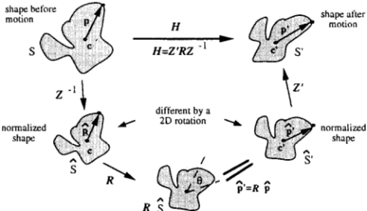
Consider a 2D shape S. It moves to another new position S’ according to the following formula (see

Figure I):

p’-

[;:I =“[-;]

+t=Hp+r

(1)

where H is a 2 x 2 transform matrix, and

p

and p’ separately stand for the corresponding points before and after motion. Equation (1) defines the afline motion model which includes translating, scaling, rotating and skewing in 2D space.

All we know as input data are two 2D shapes, S and S’. However, the one-to-one point correspondences

normalized shape 7 _{different by a} fl 2D rotation \ normalized shape

Figure 1 Normalization process of two 2D shapes that are different by an affine transformation

between them are entirely unknown. We also assume that both these shapes are complete, and there are no missing parts. Under the above conditions, our final goal is to determine the unknown transform matrix H and translation vector t.

Before describing our main algorithm, some points must be considered:

1.

2.

Camera effects, such as perspective projection or distortion, are not considered here, i.e. we do not consider how the 2D input data is obtained.

Only the case that det(H) > 0 is considered here. The problem of mirror projection, det(H) < 0, can be solved by a slight modification to the equations, and they are not discussed in this paper for simplicity.

Main algorithm

Because the 2D shape S undergoes an affine motion, the mass centre c of S must correspond to the mass centre c’ of the new shape S’. Here the mass centres are defined as:

c =+, _ss spdS; c’ =+-,, _ss s,p’dS’

(2)

Therefore, without loss of generality, the points on the object can be represented by an object-centred coordinate system. To simplify the notation, we assume that the position vectors

p

and

p’

have been separately expressed by their own object-centred coordinate systems. So, we have c = 0, c’ = 0 and t = 0. The transform described in equation (1) can now be simplified to:

p’ G Hp ₍₃₎

The 2 x 2 dispersion matrices M and M’ of shapes S and S’ can be separately defined as:

M = +,

JJ

s pprdS; M’ = &,

JJ

s, p’p’TdS’ (4)

where ISI and IS’/ are separately the areas of S and S’, and the superscript T denotes the transpose operation.

(3)

Notice the elements of the dispersion matrices; they are just equal to the second-order moments of the shapes.

After substituting equation (3) into equation (4), we have:

M’ = HMH7 ₍₅₎

The two dispersion matrices M and M’ can be separately decomposed by similarity transformation, defined as follows:

M = QAQ’ = (Qh,,2)I(QA,/2)‘- = ZIZT ₍₆₎ M’ = Q’A’QIT = (Q’R;+(Q’h;,JT = Z’ZZ’T ₍₇₎

Here Q and Q’ are orthogonal matrices and their determinants must be equal to +1 (avoiding the mirror projection). A and A’ are two diagonal matrices with non-negative elements. A = IZ,/~A,/? and A’ = R’,,,2h’,,z. I is a 3 x 3 identity matrix.

After substituting equations (6) and (7) into equation (5), we have:

Z’Z’r = HZZT H’ = (HZR ‘) (HZR T)T ₍₈₎

where R is a 2 x 2 orthogonal matrix. It is easy to observe that:

H = Z’RZ-’

₍₉₎

Equation (9) is the most important equation in this algorithm. In fact, equation (9) can be more clearly interpreted by the concept of normalization. Let us again see Figure 1. If we change the two original shapes (S and 5”) to new shapes (3 and 3’) by the following transforms:

p=z ‘p: $_z’-‘p’

₍₁₀₎

it is easy to prove that the dispersion matrices of the two new shapes 5 and i’ are both equal to an identity matrix. We may call 3 and >’ the normalized shapes.

From the description in Leu”, we know that the two normalized objects are only different by a 2D rotation matrix R. i.e.:

fi’ = Rf,

₍₁₁₎

Combining equations (3), (10) and (1 l), we have:

p’ = (Z’RZ ~‘)p = Hp ₍₁₂₎

Comparing equation (12) with equation (9), we find that both of them represent the transform matrix H by the same form Z’RZ--‘. On the other hand, the physical meaning of the orthonormal matrix R is now clearly defined. Matrix R is just the rotation difference between the two normalized objects. Because we do not consider the case that det(H) < 0 (the mirror projection). the value det (R) must be equal to 1.

Once the rotation matrix R is determined, the transform matrix H will be obtained easily by equation (9), and the whole problem is completely solved. The methods of determining R will be described later.

The above derivations can be extended directly to the

discrete-point 2D structures by slightly modifying the definitions of dispersion matrices M and M ‘:

(13) The key equation (9) is then usable

Determine the 2D rotation matrix

In this subsection, we consider two main approaches: the weighting method and the modified method. Basically. these two methods are very similar. The differences between them come from the different utilization of the normalized shapes. .$ and s’.

Weighting method

Consider a single-valued weighting function g(r). From equation (1 I). we can immediately obtain the following equation:

g(r’) fi’ =

Rk(r)fi)

(14)

where Y E 11fi11 = llfi’ll = Y’ and g(r) = a.

If we separately integrate both sides of equation (14) within the regions of 3 and s’, we will have:

E Rv, ₍₁₅₎

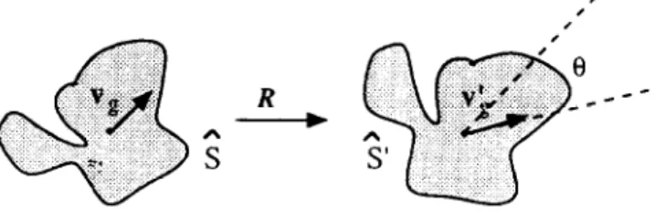
To solve the 2D rotation R, at least one weighting function I: is needed. Be sure that the function I: will not make the weighted summation vector v,~ vanish. iFrom this nonzero vector vR, we can directly estimate the’angle H representing the rotation matrix R. Figuw Z shows these ideas.

Is there any constraint that g(v) must satisfy? Here is a rule: ‘Theoretically, any single-value bounded function g(r) that will not let the weighted summ’ation vector v,? become zero will work’. For example, g(r) = YA. sin(r) or e’ are valid candidates; but g(r) = constant or l/r are inappropriate forms. Most of the time, we adopt simpler forms such as g(r) = I;’ or g(r) = Y’,2, Readers may have found that equation (I 5) is in fact a relationship .among higher (or fractional) order moments. This result seems reasonable when compared with published papers about moment invariants.

Figure 2 In the weighting method. the difference angle 0 between the two weighted-integration vectors vy and Y: can be used to estimate the rotation matrix R

(4)

When the object of interest is a discrete-point 2D structure, the weighted-integration in equation (15) should be changed to the weighted-summation, defined as:

Modified method

The method described here still uses the property of normalized objects (equation (11)); however, different to the weighting method, we no longer calculate any weighted-integration (or summation) vectors of normalized objects. On the contrary, we try to find the best matching between the two normalized shapes S and S’, then the best rotation matrix R is substituted into equation (9) to determine H. The matrix R estimated here is usually more reliable than that done by the weighting method, because the reliability of the weighting method depends upon the amplitude of vK and any position errors will directly affect the values of weighting function g(r). Therefore, we may call this new method the modl3ed method. Experiments will show its excellence in error performance.

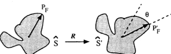
An initial best matching guess can be obtained using several simple methods (e.g. the weighting method). However, the simplest method is to detect the furthest (or the nearest) points of S and S’ and calculate their angle difference (Figure 3). Of course, we have to test several initial guesses if the furthest point of a normalized is not unique.

If the object of interest is a discrete-point 2D structure, it will be better to determine directly the one- to-one point correspondences between its normalized objects, because the number of corresponding points is finite, not like the infinite number in a continuous 2D shape. Once the correct one-to-one point correspondences are found, it will be straightforward to determine H by solving:

[P’, I . . .

/P’,l =

H[P, I .

IPNI

Discussion

(17)

In this subsection, we discuss the benefits and shortages of the two methods described above.

In the weighting method, the reliability of the estimate of 2D rotation R depends upon the amplitude

Figure 3 In the modified method, the best rotation R can be estimated by maximizing the matching ratio between R 3 and 2’. We may use the furthest points PF and P> of the two normalized shapes to guess an initial solution

Using moments to acquire motion parameters: S-C Pei and L-G Liou

of vector vn. It no longer works if its amplitude is zero. For example, vector vR of a centre-symmetrical normalized 2D shape is always zero, no matter what kind of function g is used. This makes the weighting method break down. However, because the modified method does not use weighted integration at all, the singular cases breaking the weighting method do not cause any problem when using the modified method. Of course, these improvements are only obtained by paying the price of greater computational cost.

If the normalized shape S (or 3’) is fold-symmetric (Figure 4) multiple solutions of R (and then matrix H) should be discussed. The weighting method usually fails in these cases, but the modified method does not.

CORRESPONDENCELESS

MOTION

ESTIMATION

IN 3D SPACE

In this section, we derive a method for correspondenceless motion estimation in 3D space. The object of interest considered here can be a 3D solid volume or just a collection of several discrete points. Without loss of generality, only the equations about a discrete-point 3D structure are listed here. The derivations about 3D solid volume are very similar; we just need to change the definitions of discrete moments to continuous moments.

Problem formulation

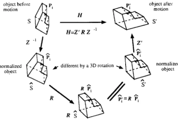
Consider a discrete-point 3D structure S. It moves to another new position S’ according to the formula:

(18)

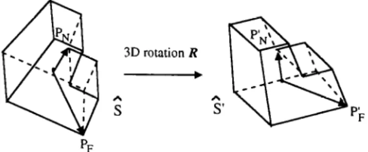
where His a 3 x 3 transform matrix, and P; and P: (for

i= l,... , IV) separately stand .for the corresponding points on S and S’. Equation (18) defines the affne motion model, which includes translating, scaling, rotating and skewing in 3D space (Figure 5).

All we know as input data are the 3D coordinates of P;s and Pis, which have been recognized as the points on the same moving object. However, the one-to-one point correspondences between S and S’ are unknown.

Figure 4 One of the ambiguity cases. If the normalized shapes are rotationally-symmetric, there may exist several possible solutions for

H

(5)

B different by a 3D rotation y normalized

object

Figure 5 Normahzdtion process of two 3D objects that are different by an afline transformation

The problem of missing points is not considered here. Under the above conditions, our final goal is to

determine the unknown transform matrix H and

translation vector T.

Before beginning our main derivations, some points must be considered:

1.

2.

We do not consider how the 3D point data is obtained (range camera or computer-aided tomography).

Only the case where det(ff) > 0 is considered here. Similar to the 2D case, the problem of mirror projection (det(H) < 0) can be solved easily by a slight modification to the equations, so they are not discussed in this paper.

Readers must have found great similarity between the 2D and 3D cases. Therefore, the 3D objects, S and S’, can also be normalized to two new objects. 3 and 3’ by defining:

k, 5 z-‘p,; p: E z’-‘p’ _I ₍₂₃₎

Here the dispersion matrices fi and h’ of the two normalized objects 3 and 3’ must be equal to a 3 x 3 identity matrix Z (Figurr 5).

From the description given by Leu”. we know that s and &?’ are different by a 3D rotation matrix R. i.e.:

k: = RF, (24)

Combining equations (19), (23) and (24), we also derive the same key equation as that in equation (9):

H = Z’RZ-1 (25)

The value det (R) must be equal to + I because det(H) is positive.

Once the rotation matrix R has been determined, the transform matrix H will be obtained easily by equation (25), and the whole problem is solved. The methods of determining R are described later.

The above derivations can easily be extended to a continuous 3D solid volume by slightly modifying the definitions of dispersion matrices M and M’:

. .

Ill

I PPTtIS: M’ = P’P”dS’ .Y

Ill

.Y’

(26)

Here, /S( and IS’1 are separately the volumes of the objects S and S’. After this modification, equatio,n (25) can also be used to determine the transform mat&x H.

Main algorithm

Without loss of generalization, we may assume that the position vectors P,s and Pis have been expressed by their own object-centred coordinate system, and equation (I 8) can now be simplified to:

Determine

the 3D rotation matrix

In this subsection, we also consider two .main approaches. the weighting method and the modified method. as in the 2D case.

P:=Hp, for i= l....,N ₍₁₉₎

The 3 x 3 dispersion matrices, M and M’, of S and S’ can be separately defined as:

(20)

Weighting method

where the superscript T denotes the transpose operation. The two dispersion matrices M and M’ can be decomposed separately by similarity transformation, defined as follows:

Consider a single-valued weighting function g(v). ‘Here the function g should satisfy the thumb’s rule described above. From equation (24). we can immediately obtain the equation:

R(@: = R(g(r,)p,) (27)

where r, e lip,ll = Ile:il c r: and ,g(r:) = g(r,) for i= l,...,N.

M = QAQ’ =

(QA/2)Z(QA,,2)T

=

.U.2TT

₍₂₁₎

If we sum both sides of equation (27) from

i= l,...,N.wehave: M’ = Q’A’Q’* = (Q’A;/2)Z(Q’A;,2)T E Z’ZZ’T (22)

Here Q and Q’ are orthogonal matrices and their determinants must be equal to +l (preventing mirror projection). A and A’ are two diagonal matrices with nonnegative elements, and Z is a 3 x 3 identity matrix.

(28)

To solve the 3D rotation R, at least two different functions (e.g. gl and g2) must be specified to acquire

(6)

two different sets of vectors, say

{V,,, Vx2}

and

{Vh,, Vi,}.

In each set, we must also make sure that its two element vectors will not be zero or parallel to each other (Figure 6).

If subset correspondences are available, as mentioned by Chaudhuri and Chatterjee14, we do not have to sum up all the weighting vectors from index 1,. , N. For example, if K( > 1) subsets of correspondences are available, we just need to sum up the g-weighted vectors in the same subset. Therefore, K different pairs of vectors, like {V,,Vh} can be obtained. So the 3D rotation estimate based on these K corresponding vectors will be more reliable. It seems that the weighting method has a greater flexibility.

Figure 7 In the modified method, the best rotation R can be

estimated by maximizing the matching ratio between R s and 3’. We

may use the furthest and nearest points {PF, PN, Pk., Pj,} of the two normalized objects to guess an initial solution

When the object of interest is a continuous 3D volume, the weighted-summation in equation (28) should be changed to the weighted-integration defined as:

rotation R, which causes a best matching between its normalized objects. This is because the number of corresponding points is infinite in this case.

v;

,L

P’I

SSJ

.!?I

g(r')P&

_Discussion

In this subsection, we discuss the benefits and short- comings of the two methods described above.

Modified method

Because the discrete-point 3D structure has a finite number of one-to-one point correspondences, the modified method described here will focus on finding the correct one-to-one point correspondence between 9 and 3’. Once the correct one-to-one point correspondences have been determined, the transform matrix H can be estimated directly by solving:

[P’, / IP’N] ‘= H [P, 1 . . . IPN] ₍₃₀₎

Many methods can serve to provide an initial guess of

The weighting method will fail when (1) any one of V,, and

VR2

is zero, or (2)

V,,

is parallel to

Vg2.

For example, the weighted-summation vector

V,

of a centre-symmetrical normalized object is always zero no matter what kind of function g is used, which makes the weighting method break down. On the other hand, the two functions, gl and g2 should be chosen appropriately for not making the opening angle between

V,I

and

VR2

too small. However, the modified method does solve these singular cases, because it never uses Ihe weighted summation (or integration). Of course, these improvements are obtained only at the cost of more computation. the correct one-to-one point correspondences. The

weighting method described earlier is one of them, but the simplest way is to find the corresponding furthest and nearest points on the two normalized objects ,$ and 3’. These points can be separately denoted by PF, P,,,,,

P> and Ph (Figure 7). From these points, we can obtain an estimate of R, which helps the later work of finding the correct correspondences. Of course, we have to test several initial guesses if these extreme points are not unique.

If the normalized 3D object 3 and i’ have some kind of rotational symmetry (Figure 8), we may have multiple solutions for R (then matrix H). In this case, the weighting method usually fails, but the modified method can solve all the possible solutions.

ERROR ANALYSIS

When the object of interest is a continuous 3D solid volume, the modified method will focus on finding the

In this section, we discuss what factors will affect the error performance of the weighting and modified

6 possible solutions Figure 6 In the weighting method, two pairs of weighted-summation

vectors are used to determine the unknown 3D rotation R between 2

and L?’

Figure 8 One of the ambiguity cases. If the normalized objects are rotationally-symmetric in 3D space, there may exist several possible solutions for H

(7)

methods. Because of the great similarity between the 2D and 3D cases, we only consider error analysis of the 3D case here. If we first assume an ideal case, where the correspondence between P,s and P:s is known, then we have:

[P’l/...iP’J = H[PiI~..IPX] (31)

If N 3 3. the transform matrix H can be solved by the equation:

IIow will the estimate of H be affected if the position vectors P,s and P:s are perturbed by noise? If the perturbed forms of these position vectors are represented by P,s and Pis, then we have the perturbed

forms of B, M, H: b=B+AB,n-i=M+AM,

I? == H + AH and fi = BI%-‘. Substituting them into equation (32) we have:

AHEI&Hz -H(AM)M-’ + (AB)B-‘H

= -H(AM)K’ + (AB)M-’ ₍₃₃₎

where the second-order errors are neglected.

We further define the relative estimation error of H as IIAHIIFlllHllF~ where

ll.IIF

is detined as the Frobenius norm. Finally, an upper bound of this relative error can be derived as:

!s

G IW~II,II~~‘lI,. + II~BIIFI~B~‘IIF

(34)

I

From equation (34) it is easy to see that if matrix M or B has an eigenvalue which is very close to zero, then the final estimated motion matrix will be very error- sensitive. A close-to-zero eigenvalue of M means that the object structure is degenerate, such as a planar patch in 3D space or a 1D line in 2D space. When the correct correspondences are available, the error performance only depends upon the structures before and after motion, which also means that the error performance will not be affected, no matter how the correct correspondences are obtained. So we know that the performance of the modified method must be the same as this ideal case.

As for the weighting method, the error sensitivity of the estimated motion matrix His quite different. Let us begin from the error-perturbed form of equation (25), i.e.:

r$=z’RZm’

(35)

where Z’=Z’+AZ’, R=(AR)R=(Z+AW) Rand

Z == Z + AZ. 0 = (Q,., R,., O,)T is the rotation vector representing the 3 x 3 matrix R. A W is an anti- symmetric matrix defined as:

0 -AR, AR,

AWz AR, 0 -A% I

(36)

-An,, AR, 0

After substituting equations (25) and (36) into the definition of AH, we have

AH- fi- Hx [(AZ’)(Z’))‘] H+ H[(Az,(Z) ~‘1

+ Z’[(AW’)R]Z-’ (37)

Similar to equation (34), we derive an upperbound of the relative error, llAHllF/ilH~iF, as follows:

relative error G w 6 /IAZ’]lF]]Z’- ’ IIF f

+ Il~-w~-‘IlF + IIAWF

(38)

From equations (21) and (22) we know /IZ-‘II, = llA,‘211, and l/Z’-‘II, = IIA~~;~ IIF. Obviously, because M = ZZr and M’ = Z’Z’T. the estimation will be also very error-sensitive when the dispersion matrix M or M’ has a close-to-zero eigenvalue. There is also an additional rotation-error term that can affect our final results.

Therefore, from equations (34) and (38), it is easy to realize that there exist some special cases whose motion parameters are inherently hard to estimate. However, readers should realize that the motion estimation of these special cases fails because the object of interest is allowed to move in 3D space in a linearly-deformable manner. For example, a moving rigid planar patch in 3D space will have an undefined expansion along its normal direction, which causes singularity.

SIMULATION

EXPERIMENTS

To test our derivations described above, several simulation experiments are designed here. The main objectives of these experiments are to prove that our methods are absolutely accurate when no position errors exist, to show that the error performance of the modified method is superior to the weighting method, and to show how the modified method solves the ambiguity problem.

Only position errors are considered in the following experiments.

Error-free cases

In this experiment, two kinds of structures are tested: a 2D continuous shape and a 3D discrete-point structure. Our main objective is to show the validity of the algorithms derived above when no position errors are introduced.

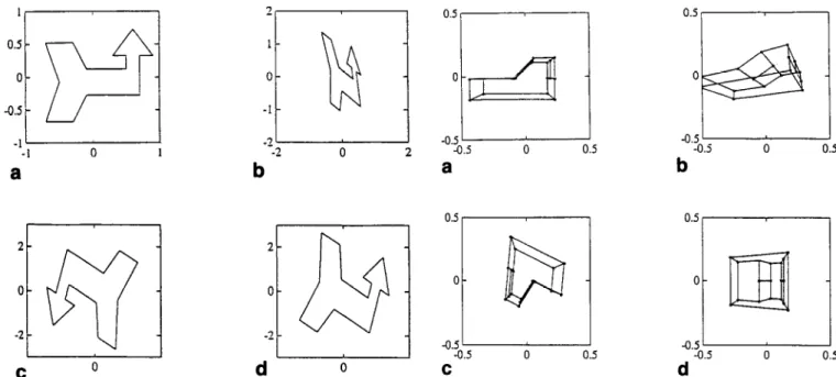
Figures 9a-d show the normalization process of 2D shapes S and S’. The shape S is contained in a rectangle of 1.6 x 1.4. Figure 9a is the shape before motion (S).

Figure 9h is the shape after motion (S’). Figure 9c is the normalized shape of S, that is 3’. Figure 9d is the normalized shape of S’, that is S. Table I lists the real and estimated motion parameters. It can be easily observed that the estimation of H is accurate. Notice

(8)

I( ₁ 0.5 0 t -0.5 -1 IIc -1 0

I

a

I 1 C 0 d- 0

Figure 9 Normalization process of a 2D continuous shape. (a) Unmoved shape S; (b) moved shape S’; (c) normalized shape S of S; (d) normalized shape S’ of S’

that the name ‘Weight: (k)’ on this table represents that the weighting function g(r) used in the weighting method is defined as g(r) = rk,

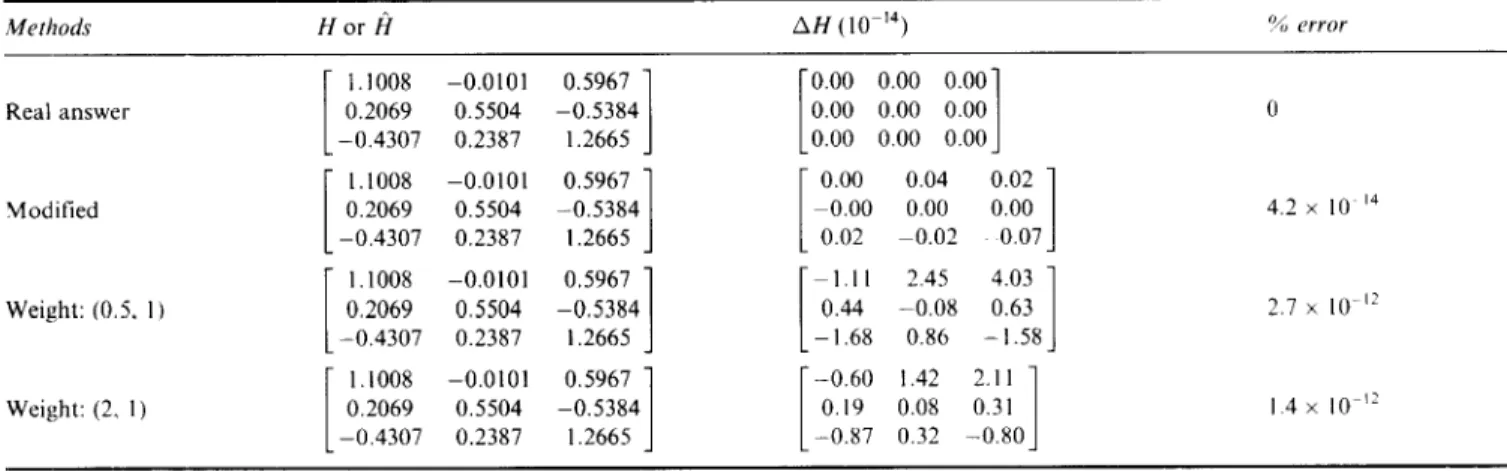
Figure lOa-d show the normalization process of a discrete-point 3D structure (only vertices are considered). The whole structure of this car-like structure is contained in a rectangle volume whose size is 4 x 2 x 2.

Figure IOa-d separately represents the object S, S’, 3 and 3’. Table 2 lists both the real and estimated motion parameters. It can easily be observed that the estimation is accurate. Notice the name ‘Weight: (a, b)’ represents that the two weighting functions g,(r) and gz(r) used in this weighting method are separately defined as

g)(r) = ra and g*(r) = rh.

From the results shown in Figure II, we find that the error performance of the modified method (assuming that correct correspondences are obtained) is consider- ably better than that of the weighting method. In fact, when the object structure is more asymmetric, the performance of the weighting method,may be better. This means that the structure of the object has a critical influence to the weighting method.

Cases when position errors exist

In this experiment, we try to show how the moditied

method is superior to the weighting method in error =k 50 performance. Here, we use the 3D discrete-point r 1 45 structure in Figure 10. Position errors are added to > 40

each point, and these errors are assumed to be 35

uniformly distributed in a small cubic whose edge $ = 30 + 0 & 25 Table 1 Listing table of the estimated motion for Figure 9

J 20

Methods Hor k AH (10@5) % error z

,u 15 $ 10 Real answer

b

5 Modified [ 0.7 -0.2 k -0.6 1.8 I [ 0.11 0.22 -0.08 -0.22

1

1.7 x IO_‘4 Lu 0 Weight: (1) 0.7 -0.2

1 [

-0.22 1.06 -0.6 1.8 -1.67 -0.67

1

1.0 x lo-‘3 Weight: (2) 0.7 -0.2 -0.22 0.61 -0.6 1.8

1 [

-0.89 -1.11

1

7.7 x lo-l4

Figure 11 Error performance of the weigtiting and modified methods. We can observe that the modified method is significantly better than the weighting method in error sensitivity

0

t4

1

Using moments to acquire motion parameters: S-C Pei and L-G Liou

-0.5 L_..-J 05. -0.5 0 0.5 -0.5 0 0.5

a

b

0.5 [I, 0.5 7, -0.5 - -0.5 0 0.5 C -0.5 - -0.5 0 0.5

d

Figure 10 Normalization process of a 3D discrete-point structure. (a) Unmoved object S; (b) moved object S’; (c) normalized object S of S; (d) normalized object 3’ of S’

lengths are all 26. In Figure 11 four curves are plotted. Each point of the curves comes from the averaging of 100 different tests under the same error level 6. The lowermost curve is the result of the modified method; the higher three curves are the results of the weighting method, whose weighting functions are gl(r) = ra and

gl(r) = rh. (a, b) represents the weighting functions in this experiment. Notice that the error percentage of the estimation is defined as IIAHIIF/IIHIIF x 100%.

0 0.02 0.04 0.06 0.08 0.10

Position error deviation 6

(9)

Table 2 Listing table of the estimated motion for Figure 10

Methods Hor 6 AH ( 10-‘4) % error

1.1008 Real answer 0.2069 -0.4307 Modified Weight: (0.5. I) 1.1008 [ 0.2069 -0.4307 [ 1.1008 0.2069 -0.4307 Weight: (2. I) I.1008 0.2069 -0.4307 -0.0101 0.5504 0.2387 -0.0101 0.5504 0.2387 -0.0101 0.5504 0.2387 -0.0101 0.5504 0.2387 0.5967 -0.5384 1.2665 I 0.5967 -0.5384 1.2665

1

0.5967 -0.5384 1.2665

1

0.5967 -0.5384 I .2665

1

0 [ -0.00 0.00 0.02 -0.02 0.04 0.00 -0.07 0.02 0.00

I

4.2 x IO I4 [ -1.1 -I 0.44 .68 I -0.08 0.86 2.45 -1.58 4.03 0.63

I

7

_. 7 x IO_ ‘? -0.60 1.42 0.19 0.08 0.31 -0.87 0.32 _2.11

I

I4 x IO_” -0.80

To provide a more clear sense about the motion estimation, some numerical results are listed in Tables 3

and 4. Notice that the performance of the weighting method in Table 3 is not so sensitive to position errors as that in Table 4, because the tested 2D shape is quite asymmetric, and only one weighting function is used in the 2D case, and the final summation vector and then the estimated rotation

R

will not be influenced by other summation vectors (comparing it only with the 3D case).

Cases when ambiguities exist

We know from earlier that the weighting method fails when ambiguity or a degenerate case happens. This Table 3 Estimation result of the 2D shapes displayed in Figure 9. Here, the error level 6 is set to 0.02

Meth0d.s H or k % error Real answer 0.7 -0.2

1

-0.6 I .8 0 Modified [ 0.7096 -0.1928 -0.578 I I .7799

1

1.58 Weight: (I ) [ 0.7168 -0.1981 -0.5806 I .7623

1

2.24 Welyht: (2) 0.7175 -0.2081 -0.5788 I .765l I 2.49

Table 4 Estimation results of the 3D object displayed in Figure 10. Here, the error level 6 is set to 0.01

Methods H or fi % error I.1008 -0.0101 0.5967 Real answer 0.2069 0.5504 -0.5384 -0.4307 0.2387 I .2665

I

0 I .0983 -0.0103 0.5964 Modified [ 0.2084 0.5500 -0.5370 --0.4332 0.2430 I .2677

I

0.3016 1.0869 0.0256 0.6250 Weight: (0.5. I) [ 11.2092 0.5539 -0.4449 0.2432 -0.5320

I

2.56 1.2561 I ,086 I 0.0342 0.6210 Weight: (2. I) 0.2071 0.5572 -0.5327

1

2.75 m~O.4430 0.238 I I .2577

experiment shows how the modified method solves the ambiguity problem. Figure 12u-d are similarly defined as in Figure 9a-d. Notice that the 20 shape we use here is symmetric to its centre. When the weighting method is used (g(r) = rk), both of the weighted summation vectors vK and vi are zeros, which makes the weighting method fail. However, the modified method can solve two possible solutions listed in Table 5. One of them

1 :P 0.5 0 -0.5 BI

-IL

I -I 0 1

a

b

2- -2-e: o- C 0

1

2L O:C& -2

1 d

0

Figure 12 Normalization process of a 2D symmetric shape. (a) Unmoved shape S; (b) moved shape S’; (c) normalized shape S of S: (d) normalized shape S’ of S’

Table 5 Listing table at the estimated motion. Note the failure of the weighting method Methods Her fi Real answer Modified # I Modified # 2 Weighting 0.7 -0.2 PO.6 _{I .8 1} [ 0.7 -0.6 -0.2 I.8

1

[ -0.7 0.2 0.6 -1.8

1

fail

(10)

corresponds to the true answer; the other is an ambiguous solution.

CONCLUSION

In this paper, we have attempted to find the motion parameters of a uniformly-deformable object in 2D or 3D space. The features representing the object of interest are allowed to be discrete points, continuous 2D shapes or a 3D solid volume. The so-called affine motion model is defined as a linearly-deformable one which must be satisfied everywhere on the object (as described in equations (1) and (18)).

As we know, we often need to solve the correspondence problem before we want to estimate the motion parameters of an object. However, this problem has been hard enough in the case of rigid motion, and is even harder in the case of deformable motion. To prevent such a difficulty, we have theoretically developed a method without using one-to-one point correspondences, and a closed-form solution has been derived. The concept of normalization is the key idea in our method.

However, it is not enough to just know that this method is accurate when no position errors exist. We should notice many other important things. For example, if position errors exist, how robust are our methods? How do the structure of the object and its associated motion parameters affect the error performance? Can our method solve all kinds of object structure and motion parameters? If not, in what cases will our methods break down? If they break down, is there any other method which can solve it? All those questions are discussed and answered in our paper.

Here, we summarize our final conclusions:

According to the derivations discussed earlier, we know that the position error sensitivity of motion parameters depends upon the dispersion matrices of the object before and after motion. The error performance is inherently bad when there exists a close-to-zero eigenvalue of the dispersion matrices. This means that the object structure is almost degenerate, and no method can estimate its motion parameters. For example, a 2D plane object in 3D space and a 1D line object in 2D space are degenerate structures. (Notice the deformation motion model we used here.)

We presented the weighting method and the modified method; the former uses distance weighting of the normalized object as its main idea, while the latter uses the characters of normalized object to solve the correspondence problem. Both the theory and experimentation indicate that the error performance of the modified method is better than that of the weighting method. However, the modified method needs more time and computational cost to determine the best matching of the normalized objects.

The modified method (especially to the discrete- point structure) can perform as well as those methods which previously know the correct correspondences.

If the normalized structure of the object of interest is symmetric to its centre, the weighting method will fail because the weighted summation vector vg (or V,) is always zero no matter what kind of weighting function g is used. But the modified method can solve this singular case, and provide all possible solutions.

Some methods using high-order moments or tensors to solve the motion parameters are in fact similar to our weighting method. We can thus predict that the error performance of such tensor methods should be comparable with the weighting method.

Although only theoretical research is presented in our paper, we can apply this result to many real applications that need point correspondences and where the objects satisfy the aftine transformation. For example, if a moving rigid planar patch is placed at a distance far from the camera, its two image shapes projected on the image plane at two different time instants will approxi- mately satisfy the 2D aftine relationship, and we can estimate the correspondence by obtaining their best- fitted aftine transformation. Another example is to estimate the 3D motion of the heart by obtaining the 3D data from CAT (computer-aided tomography), as done by Faber and Stokely”.

REFERENCES I 2 3 4 5 6 I 8

Hu, M K ‘Visual pattern recognition by moment invariants’, IRE Trans. hfor. Theory, Vol 8 (February 1962) pp 1799187 Lo, C-H and Don, H-S ‘3-D moment forms: their construction and application to object identification and positioning’, IEEE Trans. PAMI, Vol 11 No 10 (October 1989)

Yaser, S. Abu-Mostafa and Psaltis, D ‘Recognitive aspects of moment invariants’, IEEE Trans. PAMI. Vol 6 No 6 (November 1984)

Cyganski, D and Orr, J A ‘Applications of tensor theory to object recognition and orientation determination’, IEEE Trans. PAMI. Vol7 No 6 (November 1985)

Sluzek. A ‘Using moment invariants to recognize and locate partially occluded 2-D object’, Putt. Recogn. Left., Vol 7 (1988) pp 253-257

Sadjadi, -A and- Hall, E L ‘Three-dimensional moment invar- iants’, IEEE Trans. PAMI. Vol 2 No 2 (March 1980)

Arbter, K. Snyder, W E. Burkhardt, H and Hirzinger, G ‘Applications of affne-invariant Fourier descriptors to recogni- tion of 3-D objects’. IEEE Trans. PAMI, Vol 12 No 7 (July 1990) Young, T Y and Wang, Y-L ‘Analysis of three-dimensional rotation and linear shape changes’. Putt. Recogn. Lett., Vol 2 (1984) pp 239-242

Pinjo, Z, Cyganski, D and Orr. J A ‘Determination of 3-D object orientation from projections’. Part. Recogn. Let/., Vol 3 (1985)

pp 351-356

Sluzek, A ‘Identification of planar objects in 3-D space from perspective projection’. Pat/. Recogn. Left., Vol 7 (1988) pp 59- 63

Blake. A and Cipolla, R ‘Robust estimation of surface curvature from deformation of apparent controus’. Image & Vision Cornput., Vol 9 No 2 (April 1991)

Leu, G Shape normalization through compacting’, Parr. Recogn. Let/., Vol 10 (1989) pp 2433250

Lee, R, Lu, P-C and Tsai, W-H ‘Moment preserving detection of

(11)

elliptical shapes in gray-scale images’, Pa//. Recogn. Let/., Vol I I ( 1990) pp 405-4 I4

14 Chaudhuri. S and Chatterjee. S ‘Motion analysis of a homo- geneously deformable object using subset correspondences’, Ptrrr.

Recogn.. Vol 24 No 8 (1991) pp 739-745

15 Faber. T L and Stokely, E M ‘Orientation of 3-D structures in medical image’, IEEE Trms. PAMI, Vol IO No 5 (September 1988)

16 Pei, S C and Liou. L-G ‘Tracking a planar patch in 3-D space by

affine transformation in monocular and binocular v&on’, Purl.

Recogn., Vol 26 No I (1993) pp 23-3 I

I7 Pei. S C and Liou. L-G ‘Finding the motion. position and orientation of a planar patch In 3-D space from scaled-ortho- graphic projection’, PO//. Recogn., Vol 27 No I (1994) pp 9-25 I8 Tang. G Y ‘A discrete version of Green’s theorem’. IEEE Truns.

PAMI Vol 4 No 3 (May 1982)

I9 Leu. J-G ‘Computing a shape’s moments from its boundary’. Patt. Rec~ogn., Vol 24 No IO (1991) pp 949-957