Mining Fuzzy Multiple-Level Association Rules from Quantitative Data

Mining Fuzzy Multiple-Level Association Rules

from Quantitative Data

Tzung-Pei Hong*

Department of Electrical Engineering National University of Kaohsiung

Kaohsiung, 811, Taiwan, R.O.C. tphong@nuk.edu.tw

Kuei-Ying Lin and Been-Chian Chien

Graduate School of Information Engineering I-Shou University

Kaohsiung, 84008, Taiwan, R.O.C. m883331m@isu.edu.tw

Abstract

Machine-learning and data-mining techniques have been developed to turn data into useful task-oriented knowledge. Most algorithms for mining association rules identify relationships among transactions using binary values and find rules at a single-concept level. Transactions with quantitative values and items with hierarchical relationships are, however, commonly seen in real-world applications. This paper proposes a fuzzy multiple-level mining algorithm for extracting knowledge implicit in transactions stored as quantitative values. The proposed algorithm adopts a top-down progressively deepening approach to finding large itemsets. It integrates fuzzy-set concepts, data-mining technologies and multiple-level taxonomy to find fuzzy association rules from transaction data sets. Each item uses only the linguistic term with the maximum cardinality in later mining processes, thus making the number of fuzzy regions to be processed the same as the number of original items. The algorithm therefore focuses on the most important linguistic terms for reduced time complexity.

Keywords: association rule, data mining, fuzzy set, quantitative value, taxonomy.

1. Introduction

Machine-learning and data-mining techniques have been developed to turn data into

useful task-oriented knowledge [20]. Deriving association rules from transaction databases is

often the objective of data mining [1, 2, 6, 9, 10, 11, 13, 14, 26, 27]. Relationships among

items are discovered such that the presence of certain items in a transaction tends to imply the

presence of certain other items. Association rules are very broadly applied. For example, they

can be used to inform supermarket managers of what items (products) customers tend to buy

together, and thus are useful for planning and marketing activities [1, 2, 5]. More concretely,

assuming that the association rule, “if a customer buys milk, that customer is also likely to

buy bread” is mined out, the supermarket manager can then place the milk near the bread area

to prompt customers to purchase them simultaneously. The manager can also promote milk

and bread sales by grouping them during special sales so as to earn good profits for the

supermarket.

Most previous studies have concentrated on showing binary-valued transaction data.

However, transaction data in real-world applications usually consist of quantitative values, so

designing a data-mining algorithm able to deal with quantitative data presents a challenge to

workers in this research field.

In the past, Agrawal and his co-workers proposed several mining algorithms for finding

also proposed a method [27] for mining association rules from data sets using quantitative and

categorical attributes. Their proposed method first determines the number of partitions for

each quantitative attribute, and then maps all possible values of each attribute onto a set of

consecutive integers. Other methods have also been proposed to handle numeric attributes and

to derive association rules. Fukuda et al. introduced the optimized association-rule problem

and permitted association rules to contain single uninstantiated conditions on the left-hand

side [11]. They also proposed schemes for determining conditions under which rule

confidence or support values are maximized. However, their schemes were suitable only for

single optimal regions. Rastogi and Shim extended the approach to more than one optimal

region, and showed that the problem was NP-hard even for cases involving one uninstantiated

numeric attribute [23, 24].

Fuzzy set theory is being used more and more frequently in intelligent systems because

of its simplicity and similarity to human reasoning [19]. Several fuzzy learning algorithms for

inducing rules from given sets of data have been designed and used to good effect in specific

domains [3-4, 8, 12, 15-17, 25, 28-29]. Strategies based on decision trees were proposed in [7,

21-22, 25, 30-31], and Wang et al. proposed a fuzzy version space learning strategy for

managing vague information [28]. Hong et al. also proposed a fuzzy mining algorithm for

managing quantitative data [14].

knowledge from transactions stored as quantitative values. The proposed algorithm adopts a

top-down progressively deepening approach to finding large itemsets. It integrates fuzzy-set

concepts, data-mining technologies and multiple-level taxonomy to find fuzzy association

rules in given transaction data sets. Each item uses only linguistic terms with maximum

cardinality in later mining processes, thus making the number of fuzzy regions processed

equal to the number of original items. The algorithm therefore focuses on the most important

linguistic terms for reduced time complexity. The mined rules are expressed in linguistic

terms, which are more natural and understandable for human beings.

The remaining parts of this paper are organized as follows. Data mining at multiple-level

taxonomy is introduced in Section 2. Notation used in this paper is defined in Section 3. A

new fuzzy multiple-level data-mining algorithm for quantitative data is proposed in Section 4.

An example illustrating the proposed algorithm is given in Section 5. Experimental results are

shown in Section 6. Discussion and conclusions are presented in Section 7.

2. Mining at Multiple Concept Levels

The goal of data mining is to discover important associations among items such that the

presence of some items in a transaction will imply the presence of some other items. To

achieve this purpose, Agrawal and his co-workers proposed several mining algorithms based

They divided the mining process into two phases. In the first phase, candidate itemsets were

generated and counted by scanning the transaction data. If the number of an itemset appearing

in the transactions was larger than a pre-defined threshold value (called minimum support),

the itemset was considered a large itemset. Itemsets containing only one item were processed

first. Large itemsets containing only single items were then combined to form candidate

itemsets containing two items. This process was repeated until all large itemsets had been

found. In the second phase, association rules were induced from the large itemsets found in

the first phase. All possible association combinations for each large itemset were formed, and

those with calculated confidence values larger than a predefined threshold (called minimum

confidence) were output as association rules.

Most algorithms for association rule mining focused on finding association rules on the

single-concept level. However, mining multiple-concept-level rules may lead to discovery of

more specific and important knowledge from data. Relevant data item taxonomies are usually

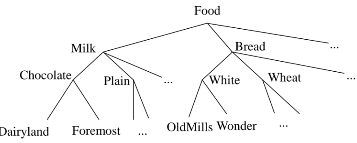
predefined in real-world applications and can be represented using hierarchy trees. Terminal

nodes on the trees represent actual items appearing in transactions; internal nodes represent

Figure 1: An example taxonomy

In Figure 1, the root node is at level 0, the internal nodes representing categories (such as

“milk”) are at level 1, the internal nodes representing flavors (such as “chocolate”) are at level

2, and the terminal nodes representing brands (such as “Foremost”) are at level 3. Only

terminal nodes appear in transactions.

Han and Fu proposed a method for finding level-crossing association rules at multiple

levels [13]. Nodes in predefined taxonomies are first encoded using sequences of numbers

and the symbol "*" according to their positions in the hierarchy tree. For example, the internal

node "Milk" in Figure 1 would be represented by 1**, the internal node "Chocolate" by 11*,

and the terminal node "Dairyland" by 111. A top-down progressively deepening search

approach is used and exploration of “level-crossing” association relationships is allowed.

Candidate itemsets on certain levels may thus contain other-level items. For example,

candidate 2-itemsets on level 2 are not limited to containing only pairs of large items on level

Food

...

Milk

Plain

Chocolate

...

...

White

Wheat

Dairyland

Foremost

OldMills Wonder

Bread

...

...

2. Instead, large items on level 2 may be paired with large items on level 1 to form candidate

2-itemsets on level 2 (such as {11*, 2**}).

3. Notation

Formally, the process by which individuals from a universal set X are determined to be

either members or non-members of a crisp set can be defined by a mapping function

containing 0 and 1. This kind of function can be generalized such that the values assigned to

the elements of the universal set fall within specified ranges, referred to as the membership

grades of these elements in the set. Larger values denote higher degrees of set membership.

Such a function is called the membership function,

µ

defined. This function is represented by

µ

where [0, 1] denotes the interval of real numbers from 0 to 1, inclusive. The function can also

be generalized to any real interval instead of [0,1].

A special notation is often used in the literature to represent fuzzy sets. Assume that x1 to

A

=

µ

/

x

+

µ

/

x

+

...

+

µ

/

x

The following symbols are used in our proposed algorithm:

n: the number of transactions;

i

D : the i-th transaction, 1≤i≤n;

x: the number of levels in a given taxonomy. k

m : the number of items (nodes) at level k, 1≤k≤x ; k

j

I : the j-th item on level k, 1≤k≤x; 1≤j≤ mk;

k j

h : the number of fuzzy regions forIkj; k

jl

R : the l-th fuzzy region of Ikj, 1≤l≤hkj;

k ij

v : the quantitative value ofIkj inDi;

k ij

f

ijl

f : the membership value of Di in region k jl R ;

k jl

count : the summation of fijlk, i=1 to n;

max-countkj: the maximum count value among countjlvalues, l=1 to

k j

h ;

max-Rk_j: the fuzzy region of I_ik with max−countk_j;

λ

k r

C : the set of candidate itemsets with r items on level k;

k r

L : the set of large itemsets with r items on level k.

4. The Multiple-level Fuzzy Data-mining Algorithm

The proposed mining algorithm integrates fuzzy set concepts, data mining and

multiple-level taxonomy to find fuzzy association rules in a given transaction data set. Details

of the proposed mining algorithm are given below.

The fuzzy mining algorithm using taxonomy:

INPUT: A body of n quantitative transaction data, a set of membership functions, predefined

taxonomy, a predefined minimum support value α, and a predefined confidence

valueλ.

OUTPUT: A set of fuzzy multiple-level association rules.

STEP 1: Encode the predefined taxonomy using a sequence of numbers and the symbol "*",

with the t-th number representing the branch number of a certain item on level t.

STEP 2: Translate the item names in the transaction data according to the encoding scheme.

STEP 3: Set k=1,where k is used to store the level number being processed.

the count of each group in the transactions and remove the groups with counts less than α; Denote the j-th group total on level k in transaction Di as

k ij v .

STEP 5: Transform the quantitative valuev_ijk of each transaction datum Di, (i=1 to n) for each

encoded group name Ik_j into a fuzzy set f_ijk represented as

        + + + _k jh k ijh k j k ij k j k ij R f R f R f .... 2 2 1 1

by mapping v_ijk from the given membership functions,

where h is the number of fuzzy regions for Ik_j, k jl

R is the l-th fuzzy region of Ik_j,

h l≤

≤

1 , and f_ijlk isv_ijk’s fuzzy membership value in regionRk_jl.

STEP 6: Calculate the scalar cardinality of each fuzzy region Rk_jl in the transaction data:

∑

STEP 7: Find max-

(

)

jl h l k j MAX count count k j 1 = = , for j= 1 to mk, where k j

h is the number of fuzzy regions for Ik_j and mk is the number of items (nodes) on level k. Let max- k

j

R be

the region with max- k j

count for item Ik_j, which will be used to represent the fuzzy

characteristic of item Ik_j in later mining processes.

STEP 8: Check whether the value max- k j

count of a region max- k j

R , j=1 to mk, is larger than

or equal to the predefined minimum support value α . If a region max- k j

R is equal

to or greater than the minimum support value, put it in the large 1-itemsets ( k

L1) at

level k. That is,

{

}

STEP 10: Generate the candidate set k C2 from 1 1 L , 2 1 L , …, _Lk 1 to find “level-crossing”

large itemsets. Each 2-itemset in k

C2 must contain at least one item in

k

L1 and the

other item may not be its ancestor in the taxonomy. All possible 2-itemsets are

collected in k

C2.

STEP 11: For each newly formed candidate 2-itemset s with items (s1, s2) in C2k:

(a) Calculate the fuzzy value of s in each transaction datum D_i as fis = fis₁Λfis₂ ,

where j

is

f is the membership value of D_i in region sj. If the minimum operator is

used for the intersection, then fis =min(fis1,fis2).

(b) Calculate the scalar cardinality of s in the transaction data as:

counts=

∑

(c) If countsis larger than or equal to the predefined minimum support value

α

k

L2.

STEP 12: Set r=2, where r is used to represent the number of items stored in the current large

itemsets.

STEP 13: If k r

L is null, then set k=k+1 and go to STEP 4; otherwise, do the next step.

STEP 14: Generate the candidate set k r

C+1 from

k r

L in a way similar to that in the apriori

algorithm [1]. That is, the algorithm first joins k r

L and k r

L , assuming that r-1

items in the two itemsets are the same and the other one is different. The different

ancestors or descendants of one another. Store in k r

C+1all itemsets having all their

sub- r- itemsets in k r

L .

STEP 15: For each newly formed (r+1)-itemset s with items (s1, s2, …,sr+1) in Crk+1:

(a) Calculate the fuzzy value of s in each transaction datum D_i as

r is is is is

f

f

f

f

=

Λ

Λ

...

Λ

1 , where fisj is the membership value of Di in region

sj. If the minimum operator is used for the intersection, then isj

r j is

Min

f

f

=

(b) Calculate the scalar cardinality of s in the transaction data as:

counts=

∑

(c) If countsis larger than or equal to the predefined minimum support value

α

k r

L+1.

STEP 16: Set r=r+1 and go to STEP 13.

STEP 17: Construct the fuzzy association rules for all large q-itemset s containing items

(

)

(a) Form all possible association rules as:

k q k k s s s s s1Λ...Λ ₋1Λ ₊1Λ...Λ → , k=1 to q.

(b) Calculate the confidence values of all association rules using the formula:

∑

∑

confidence thresholdλ.

The rules output after STEP 18 can serve as meta-knowledge concerning the given

transactions. As in conventional mining algorithms, the parameters α and λ are

determined by users depending on their requirements. But the values could be given smaller

than those given in the conventional mining algorithms since the fuzzy count of each item in

each transaction is equal to or less than 1.

As described in the algorithm, Step 5 uses membership functions to transform each

quantitative value into a fuzzy set in linguistic terms. The set of discrete states can thus be

reduced. Also, the knowledge derived in Step 18 can be represented by fuzzy linguistic terms,

and easily understandable by human beings. In Step 7, each item uses only the linguistic term

with the maximum cardinality in later mining processes, making the number of fuzzy regions

to be processed the same as the number of original items. The algorithm therefore focuses on

the most important linguistic terms, which reduces its time complexity. In Steps 8 to 18, a

mining process using fuzzy counts is performed to progressively find fuzzy large itemsets and

fuzzy multiple-level association rules.

5. An Example

is a simple example to show how the proposed algorithm generates association rules from

quantitative transactions using taxonomy. The data set includes the six transactions shown in

Table 1.

Table 1. Six example transactions

TID Items

D1 (Dairyland chocolate milk, 1); (Foremost chocolate milk, 4);

(Old Mills white bread, 4); (Wonder white bread, 6);

(Present chocolate cookies, 7); (Linton green tea beverage, 7). D2 (Dairyland chocolate milk, 3); (Foremost chocolate milk, 3);

(Dairyland plain milk, 1); (Old Mills wheat bread, 5); (Wonder wheat bread, 3); (present lemon cookies, 4) (77 lemon cookies, 4).

D3 (Old Mills white bread, 7); (Old Mills wheat bread, 8);

(77 chocolate cookies, 5); (77 lemon cookies, 4).

D4 (Dairyland chocolate milk, 2); (Old Mills white bread, 5);

(77 chocolate cookies, 5).

D5 (Old Mills white bread, 5); (Wonder wheat bread, 4).

D6 (Dairyland chocolate milk, 3); (Foremost chocolate milk, 10);

(Linton black tea beverage, 3); (Nestle black tea beverage, 9)

Each transaction includes a transaction ID and some purchased items. Each item is

represented by a tuple (item name, item amount). For example, the fifth transaction consists

of five units of Old Mills white bread and four units of Wonder wheat bread. Assume the

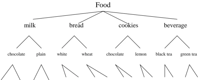
The food in Figure 2 falls into four classes: milk, bread, cookie and beverage. Milk can

be further classified into chocolate milk and plain milk. There are two brands of chocolate

milk, Dairyland and Foremost. The other nodes can be similarly explained.

Assume also that the fuzzy membership functions are the same for all the items and are

as shown in Figure 3.

Figure 3. The membership functions used in the example

Food

milk

bread

cookies

beverage

chocolate plain white wheat chocolate lemon black tea green tea

Dairyland Foremost Dairyland Foremost Old Mills Wonder Old Mills Wonder Present 77 Present 77 Linton Nestle Linton Nestle

Figure 2. The predefined taxonomy

0 1 6 11

Low Middle High

1

0 Membership value

In the example, amounts are represented by three fuzzy regions: Low, Middle and High.

Thus, three fuzzy membership values are produced for each item amount according to the

predefined membership functions. For the transaction data in Table 1, the proposed fuzzy

mining algorithm proceeds as follows.

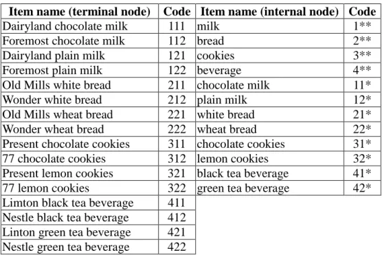
STEP 1: Each item name is first encoded using the predefined taxonomy. Results are

shown in Table 2.

Table 2. Codes of item names

Item name (terminal node) Code Item name (internal node) Code

Dairyland chocolate milk 111 milk 1**

Foremost chocolate milk 112 bread 2**

Dairyland plain milk 121 cookies 3**

Foremost plain milk 122 beverage 4**

Old Mills white bread 211 chocolate milk 11*

Wonder white bread 212 plain milk 12*

Old Mills wheat bread 221 white bread 21*

Wonder wheat bread 222 wheat bread 22*

Present chocolate cookies 311 chocolate cookies 31*

77 chocolate cookies 312 lemon cookies 32*

Present lemon cookies 321 black tea beverage 41*

77 lemon cookies 322 green tea beverage 42*

Limton black tea beverage 411 Nestle black tea beverage 412 Linton green tea beverage 421 Nestle green tea beverage 422

For example, the item “Foremost chocolate milk” is encoded as ‘112’, in which the first

digit ‘1’ represents the code ‘milk’ on level 1, the second digit ‘1’ represents the flavor

STEP 2: All transactions shown in Table 1 are then encoded using the above coding

scheme; the results are shown in Table 3.

Table 3. Encoded transaction data in the example

TID ITEMS D1 (111, 1) (112, 4) (211, 4) (212, 6) (311, 7) (421, 7) D2 (111, 3) (112, 3) (121, 1) (221, 5) (222, 3) (322, 4) (321, 4) D3 (211, 7) (221,8) (312, 5) (322, 7) D4 (111, 2) (211, 5) (312, 5) D5 (211, 5) (222 ,4) D6 (111, 3) (112, 10) (411, 3) (412, 9)

STEP 3: k is initially set at 1, where k is used to store the level number being processed.

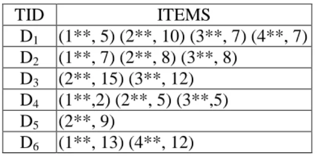
STEP 4: All the items in the transactions are first grouped on level one. Take the items in

transaction D1 as an example. The items (111, 1) and (112, 4) are grouped into (1**, 5).

Results for all the transaction data are shown in Table 4.

Table 4. Level-1 representation in the example

TID ITEMS D1 (1**, 5) (2**, 10) (3**, 7) (4**, 7) D2 (1**, 7) (2**, 8) (3**, 8) D3 (2**, 15) (3**, 12) D4 (1**,2) (2**, 5) (3**,5) D5 (2**, 9) D6 (1**, 13) (4**, 12)

The count of each group is then calculated. Assume in this example, α is set at 2.1.

STEP 5: The quantitative values of the items on level 1 are represented using fuzzy sets.

Take the first item in transaction D5 as an example. The amount “9” is mapped to the

membership function Low in Figure 3 with value 0, to the membership function Middle with

value 0.4, and to the membership function High with value 0.6. The fuzzy set transformed is then represented as 0.0 0.4 0.6 ₎

(

High Middle

Low+ +

. This step is repeated for the other items, and the

results are shown in Table 5, where the notation item.term is called a fuzzy region.

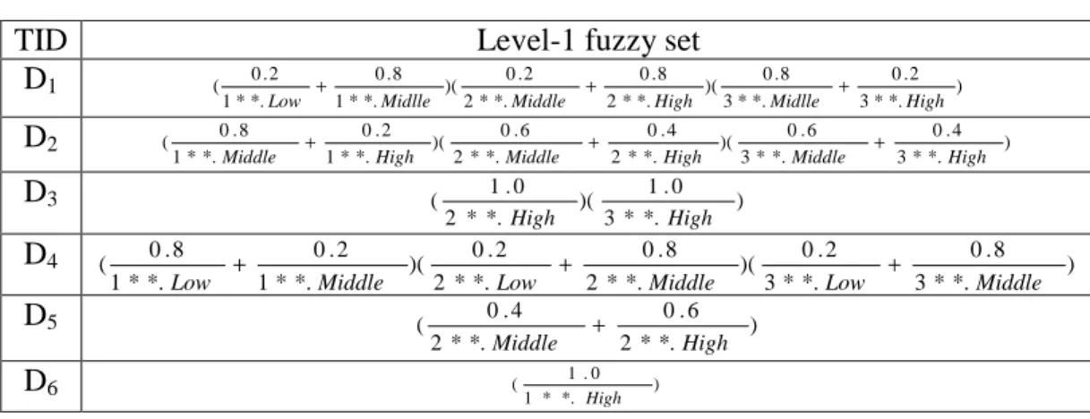
Table 5. The level-1 fuzzy sets transformed from the data in Table 4

TID Level-1 fuzzy set

D1 ) *. * 3 2 . 0 *. * 3 8 . 0 )( *. * 2 8 . 0 *. * 2 2 . 0 )( *. * 1 8 . 0 *. * 1 2 . 0 ( High Midlle High Middle Midlle Low + + + D2 ) *. * 3 4 . 0 *. * 3 6 . 0 )( *. * 2 4 . 0 *. * 2 6 . 0 )( *. * 1 2 . 0 *. * 1 8 . 0 ( High Middle High Middle High Middle + + + D3 ) *. * 3 0 . 1 )( *. * 2 0 . 1 ( High High D4 ) *. * 3 8 . 0 *. * 3 2 . 0 )( *. * 2 8 . 0 *. * 2 2 . 0 )( *. * 1 2 . 0 *. * 1 8 . 0 ( Middle Low Middle Low Middle Low + + + D5 ) *. * 2 6 . 0 *. * 2 4 . 0 ( High Middle + D6 ) *. * 1 0 . 1 ( High

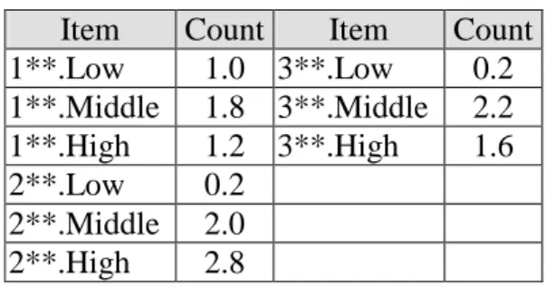
STEP 6: The scalar cardinality of each fuzzy region in the transactions is calculated as

the count value. Take the fuzzy region 1**.Middle as an example. Its scalar cardinality = (0.8

+ 0.8 + 0.0 + 0.2 + 0.0 + 0.0) = 1.8. This step is repeated for the other regions, and the results

Table 6. The counts of the level-1 fuzzy regions

Item Count Item Count

1**.Low 1.0 3**.Low 0.2 1**.Middle 1.8 3**.Middle 2.2 1**.High 1.2 3**.High 1.6 2**.Low 0.2 2**.Middle 2.0 2**.High 2.8

STEP 7. The fuzzy region with the highest count among the three possible regions for

each item is found. Take item ‘1**’ as an example. Its count is 1.0 for Low, 1.8 for Middle,

and 1.2 for High. Since the count for Middle is the highest among the three counts, the region

Middle is thus used to represent item ‘1**’ in later mining processes. This step is repeated for

the other items, “Middle” is chosen for 3**, and "high" is chosen for 2**.

STEP 8. The count of any region selected in STEP 7 is checked against the predefined

minimum support value α . Assume in this example,α is set at 2.1. Since all the count values

of 2**.High and 3**.Middle are larger than 2.1, these items are put in 1 1

L (Table 7).

Table 7. The set of large 1-itemsets ( 1 1

L ) for level one in this example

Itemset

count

2**.High 2.8

3**.Middle 2.2

STEP 10: The candidate set 1 2

C is generated from 1 1

L as (2**.High, 3**.Middle)

STEP 11. The following substeps are done for each newly formed candidate 2-itemset in

1 2 C :

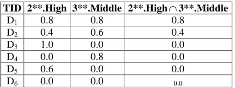
(a) The fuzzy membership values of each transaction data for the candidate 2-itemsets are

calculated. Here, the minimum operator is used for intersection. Take (2**.High,

3**.Middle) as an example. The derived membership value of (2**.High, 3**.Middle) for

transaction D2 is calculated as: min(0.4, 0.6)=0.4. The results for the other transactions are

shown in Table 8.

Table 8. The membership values for 2**.HighΛ3**.Middle

TID 2**.High 3**.Middle 2**.High∩3**.Middle

D1 0.8 0.8 0.8 D2 0.4 0.6 0.4 D3 1.0 0.0 0.0 D4 0.0 0.8 0.0 D5 0.6 0.0 0.0 D6 0.0 0.0 0.0

(b) The scalar cardinality (count) of each candidate 2-itemset in 1 2

C is calculated. Results for

this example are shown in Table 9.

Table 9. The counts of the 2-itemsets at level 1

Itemset

Count

(c) Since the count of itemset is not larger than the predefined minimum support value 2.1,

thus 1 2

L is null.

STEP 12: r is set at 2, where r is used to store the number of items kept in the current

itemsets.

STEP 13: Since L is null, k=k+1=2 and STEP 4 is done. The results for level 2 are 12

shown in Table 10.

Table 10. The set of level-2 large itemsets in the example

Itemset

Count

21*.Middle 2.6 31*.Middle 2.4

The results for level 3 are shown in Table 11.

Table 11. The set of level-3 large itemsets in the example

Itemset

Count

111.Low 3.0

211.Middle 3.0

111.Low, 3**.Middle 2.2

STEP 17: The association rules are constructed for each large itemset using the

following substeps.

(a) The possible association rules for the itemsets found are formed as follows:

If 3** = Middle, then 111 = Low.

If 111 = Low, then 3** = Middle.

(b) The confidence values of the above two possible association rules are then

calculated. Take the first association rule as an example. The count of

3**.Middle∩111.Low is 2.2 and the count of 3**.Middle is 2.2. The confidence

value for the association rule "If 3** = Middle, then 111 = Low" is calculated as:

∑

∑

2

.

2

2

.

2

Results for the two rules are shown below.

If 3** = Middle, then 111 = Low, with confidence 1.0.

If 111 = Low, then 3** = Middle, with confidence 0.73.

STEP 18: The confidence values of the possible association rules are checked against the

predefined confidence thresholdλ. Assume the given confidence thresholdλ is set at 0.7.

1. If 3** = Middle, then 111= Low, with a confidence value 1.0.

2. If 111 = Low, then 3** = Middle, with a confidence value 0.73.

These two rules can then serve as meta-knowledge concerning the given transactions.

6. Experimental Results

The section reports on experiments made to show the performance of the proposed

approach. There were implemented in C on a Pentium-III 700 Personal Computer. The

number of levels was set at 3. There were 64 purchased items (terminal nodes) on level 3, 16

generalized items on level 2, and 4 generalized items on level 1. Each non-terminal node had

four branches. Only the terminal nodes could appear in transactions.

Data sets with different numbers of transactions were run by the proposed algorithm. In

each data set, numbers of purchased items in transactions were first randomly generated. The

purchased items and their quantities in each transaction were then generated. An item could

not be generated twice in a transaction.

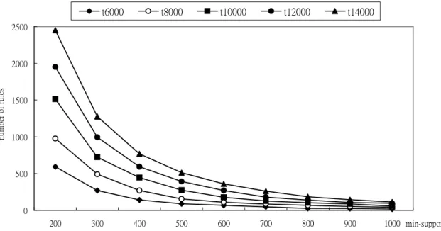
Experiments were first performed to compare various numbers of transactions. The

relationships between numbers of rules mined and minimum support values along with

minimum confidence value set at 0.7 are shown in Figure 4. The execution-time relationships

are shown in Figure 5.

Figure 4. A comparison of various numbers of transactions.

Figure 5. Execution times for various numbers of transactions.

0 500 1000 1500 2000 2500 200 300 400 500 600 700 800 900 1000 min-support nu m be r of r ul es t6000 t8000 t10000 t12000 t14000 0 20 40 60 80 100 120 140 160 200 300 400 500 600 700 800 900 1000 min-support ti m e( se co nd s) t6000 t8000 t10000 t12000 t14000

From Figure 4, it is easily seen that numbers of rules mined increase along with increase

of transaction numbers. This is very reasonable since more transactions will increase the

probability of large itemsets for a certain minimum support threshold (transaction number, not

transaction ratio). Execution times also increase along with increase of transaction numbers.

The fuzzy data-mining (FDM) method proposed in [14] was experimentally shown to

have a better effect than that with crisp partitions in [18]. Experiments were then performed to

only compare the proposed approach and the fuzzy data-mining (FDM) method to show the

effect of taxonomy. The fuzzy data-mining method proposed in [14] directly mined fuzzy

association rules from purchased items in transactions and did not utilize the taxonomy

information in the mining process. The relationships between numbers of rules mined and

minimum confidence values for an average of 10 purchased items in 6000 transactions and a

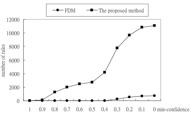
Figure 6. A comparison of the proposed method and FDM.

From Figure 6, it is easily seen that the numbers of rules by the proposed mining

algorithm are greater than those by FDM. The taxonomic structures can gather purchased

items into general classes, thus being able to generating additional large itemsets. The large

amounts of rules may, however, cause humans hard to interpret them. Thus, the support and

the confidence values in the proposed algorithm can be set at a higher value than those set by

FDM. For example, when the minimum support value is set at 1000, the number of rules can

be reduced to below 250 (from Figure 4).

7. Discussion and Conclusions

In this paper, we have proposed a fuzzy multiple-level data-mining algorithm that can

process transaction data with quantitative values and discover interesting patterns among

0 2000 4000 6000 8000 10000 12000 1 0.9 0.8 0.7 0.6 0.5 0.4 0.3 0.2 0.1 0 min-confidence nu m be r of r ul es

them. The rules thus mined exhibit quantitative regularity on multiple levels and can be used

to provide suggestions to appropriate supervisors. Compared to conventional crisp-set mining

methods for quantitative data, our approach gets smoother mining results due to its fuzzy

membership characteristics. The mined rules are expressed in linguistic terms, which are more

natural and understandable for human beings. The proposed mining algorithm can also be

degraded into a conventional non-fuzzy mining algorithm by assigning a single membership

function with values always equal to 1 for quantity larger than 0.

When compared to fuzzy mining methods, which take all fuzzy regions into

consideration, our method achieves better time complexity since only the most important

fuzzy term is used for each item. If all fuzzy terms are considered, the possible combinational

searches are large. Therefore, a trade-off exists between rule completeness and time

complexity.

Our proposed algorithm does not find association rules for items on the same paths in

given hierarchy trees. Such rules can however be found to analyze interesting behavior among

these items by slightly modifying the proposed algorithm. For example, it may be that a

certain brand of milk is found to be the most popular for its chocolate flavor from a rule that

states that if the brand of milk has high sales figures, then chocolate-flavored milk also has

high sales figures.

interest. The rules thus mined can therefore satisfy users' requirements. For example, users

can require that only items with high sales quantities are mined, which would greatly reduce

the mining time.

Although the proposed method works well in data mining for quantitative values, it is

just a beginning. There is still much work to be done in this field. In the future, we will first

extend our proposed algorithm to resolve the two problems stated above. Our method also

assumes that membership functions are known in advance. In [15-17], we proposed some

fuzzy learning methods to automatically derive membership functions. We will therefore

attempt to dynamically adjust the membership functions in the proposed mining algorithm to

avoid the bottleneck of membership function acquisition. We will also attempt to design

specific data-mining models for various problem domains.

Acknowledgment

The authors would like to thank the anonymous referees for their very constructive

comments. This research was supported by the National Science Council of the Republic of

China under contract NSC89-2213-E-214-003.

References

massive databases,“ The 1993 ACM SIGMOD Conference on Management of Data,

Washington DC, USA, 1993, pp. 207-216.

[2] R. Agrawal, T. Imielinksi and A. Swami, “Database mining: a performance perspective,”

IEEE Transactions on Knowledge and Data Engineering, Vol. 5, No. 6, 1993, pp.

914-925.

[3] A. F. Blishun, “Fuzzy learning models in expert systems,” Fuzzy Sets and Systems, Vol. 22,

No. 1, 1987, pp. 57-70.

[4] L. M. de Campos and S. Moral, “Learning rules for a fuzzy inference model,” Fuzzy Sets

and Systems, Vol. 59, No. 2, 1993, pp. 247-257.

[5] R. L. P. Chang and T. Pavlidis, “Fuzzy decision tree algorithms,” IEEE Transactions on

Systems, Man and Cybernetics, Vol. 7, No. 1, 1977, pp. 28-35.

[6] M. S. Chen, J. Han and P. S. Yu, “Data mining: an overview from a database perspective,”

IEEE Transactions on Knowledge and Data Engineering, Vol. 8, No. 6, 1996, pp.

866-883.

[7] C. Clair, C. Liu and N. Pissinou, “Attribute weighting: a method of applying domain

knowledge in the decision tree process,” The Seventh International Conference on

Information and Knowledge Management, Bethesda, Maryland, USA, 1998, pp. 259-266.

[8] M. Delgado and A. Gonzalez, “An inductive learning procedure to identify fuzzy

[9] A. Famili, W. M. Shen, R. Weber and E. Simoudis, "Data preprocessing and intelligent

data analysis," Intelligent Data Analysis, Vol. 1, No. 1, 1997, pp. 3-23.

[10] W. J. Frawley, G. Piatetsky-Shapiro and C. J. Matheus, “Knowledge discovery in

databases: an overview,” The AAAI Workshop on Knowledge Discovery in Databases,

Anaheim, CA, 1991, pp. 1-27.

[11] T. Fukuda, Y. Morimoto, S. Morishita and T. Tokuyama, "Mining optimized association

rules for numeric attributes," The Fifteenth ACM SIGACT-SIGMOD-SIGART

Symposium on Principles of Database Systems, Montreal, Canada, 1996, pp. 182-191.

[12] A. Gonzalez, “A learning methodology in uncertain and imprecise environments,”

International Journal of Intelligent Systems, Vol. 10, No. 3, 1995, pp. 357-371.

[13] J. Han and Y. Fu, “Discovery of multiple-level association rules from large databases,”

The International Conference on Very Large Databases, Zurich, Switzerland, 1995, pp.

420 -431.

[14] T. P. Hong, C. S. Kuo and S. C. Chi, "A data mining algorithm for transaction data

with quantitative values," Intelligent Data Analysis, Vol. 3, No. 5, 1999, pp. 363-376.

[15] T. P. Hong and J. B. Chen, "Finding relevant attributes and membership functions,"

Fuzzy Sets and Systems, Vol.103, No. 3, 1999, pp. 389-404.

[16] T. P. Hong and J. B. Chen, "Processing individual fuzzy attributes for fuzzy rule

[17] T. P. Hong and C. Y. Lee, "Induction of fuzzy rules and membership functions from

training examples," Fuzzy Sets and Systems, Vol. 84, No. 1, 1996, pp. 33-47.

[18] T. P. Hong, C. S. Kuo and S. C. Chi, "Trade-off between time complexity and

number of rules for fuzzy mining from quantitative data," International Journal of

Uncertainty, Fuzziness, and Knowledge-based Systems, Vol. 9, No. 5, 2001, pp.

587-604.

[19] A. Kandel, Fuzzy Expert Systems, CRC Press, Boca Raton, 1992, pp. 8-19.

[20] R. S. Michalski, I. Bratko and M. Kubat, Machine Learning and Data Mining: Methods

and Applications, John Wiley & Sons Ltd, England, 1998.

[21] J. R. Quinlan, “Decision tree as probabilistic classifier,” The Fourth International

Machine Learning Workshop, Morgan Kaufmann, San Mateo, CA, 1987, pp. 31-37.

[22] J. R. Quinlan, C4.5: Programs for Machine Learning, Morgan Kaufmann, San Mateo,

CA, 1993.

[23] R. Rastogi and K. Shim, "Mining optimized association rules with categorical and

numeric attributes," The 14th IEEE International Conference on Data Engineering,

Orlando, 1998, pp. 503-512.

[24] R. Rastogi and K. Shim, "Mining optimized support rules for numeric attributes," The

15th IEEE International Conference on Data Engineering, Sydney, Australia, 1999, pp.

[25] J. Rives, “FID3: fuzzy induction decision tree,” The First International Symposium on

Uncertainty, Modeling and Analysis, University of Maryland, College Park, Maryland,

1990, pp. 457-462.

[26] R. Srikant, Q. Vu and R. Agrawal, “Mining association rules with item constraints,” The

Third International Conference on Knowledge Discovery in Databases and Data Mining,

Newport Beach, California, August 1997, pp.67-73.

[27] R. Srikant and R. Agrawal, “Mining quantitative association rules in large relational

tables,” The 1996 ACM SIGMOD International Conference on Management of Data,

Monreal, Canada, June 1996, pp. 1-12.

[28] C. H. Wang, T. P. Hong and S. S. Tseng, “Inductive learning from fuzzy examples,” The

Fifth IEEE International Conference on Fuzzy Systems, New Orleans, 1996, pp. 13-18.

[29] C. H. Wang, J. F. Liu, T. P. Hong and S. S. Tseng, “A fuzzy inductive learning strategy

for modular rules,” Fuzzy Sets and Systems, Vol. 103, No. 1, 1999, pp. 91-105.

[30] R. Weber, “Fuzzy-ID3: a class of methods for automatic knowledge acquisition,” The

Second International Conference on Fuzzy Logic and Neural Networks, Iizuka, Japan,

1992, pp. 265-268.

[31] Y. Yuan and M. J. Shaw, “Induction of fuzzy decision trees,” Fuzzy Sets and Systems, Vol.

69, No. 2, 1995, pp. 125-139.