A Study of the Economic Efficiencies in East European Countries Using Semiparametric Approaches

行政院國家科學委員會

獎勵人文與社會科學領域博士候選人撰寫博士論文

成果報告

A study of the economic efficiencies in East

European countries using semiparametric approaches

核 定 編 號 ： NSC 98-2420-H-004-174-DR 獎 勵 期 間 ： 98 年 08 月 01 日至 99 年 07 月 31 日 執 行 單 位 ： 國立政治大學金融研究所 指 導 教 授 ： 黃台心 博 士 生 ： 陳冠臻 公 開 資 訊 ： 本計畫涉及專利或其他智慧財產權，2 年後可公開查詢

中 華 民 國 100 年 07 月 21 日

國 立 政 治 大 學 金 融 系

博 士 論 文

指導教授：黃 台 心 博士

探討半參數隨機邊界模型的技術與配置效率之

一致性估計方法

研究生：陳冠臻

中華民國九十九年六月十日

探討半參數隨機邊界模型的技術與配置效率之

一致性估計方法

摘要

傳統參數隨機成本邊界模型需事先假設其函數型態，但真正的函數型態未 知，若是假設錯誤的函數型態可能存在模型設定誤差，另外過去估計成本函數 時，大多著重於技術效率的衡量，而忽略配置效率，如此一來，將導致模型參數 估計產生偏誤，影響後來效率的計算。基於上述的問題，本研究將應用半參數隨 機成本邊界模型且同時考量技術效率與配置效率，不但函數設定具有彈性且能正 確的衡量效率值，然而在考量配置效率的衡量後，增加模型估計的困難度，使得 估計收斂不易，因此本研究提出一個五階段的估計步驟，應用蒙地卡羅模擬進行 分析，該估計步驟不但能簡化估計且能得到技術與配置效率的一致性估計。最後 則將本研究提出的估計方法應用在實證研究上，探討 14 個東歐國家在轉型期間 其技術與配置效率的衡量，使用不平衡縱橫資料，共 340 家商業銀行進行實證分 析。 關鍵字: 半參數成本邊界、核估計式、影子價格、技術效率、配置效率

Consistent Estimation of Technical and Allocative Efficiencies for a

Semiparametric Stochastic Cost Frontier with Shadow Input Prices

Abstract

Conventional parametric stochastic cost frontier models are likely to suffer from biased inferences due to misspecification and the ignorance of allocative efficiency (AE). To fill up the gap in the literature, this article proposes a semiparametric stochastic cost frontier with shadow input prices that combines a parametric portion with a nonparametric portion and that allows for the presence of both technical efficiency (TE) and AE. The introduction of AE and the nonparametric function into the cost function complicates substantially the estimation procedure. We develop a new estimation procedure that leads to consistent estimators and valid TE and AE measures, which are proved by conducting Monte Carlo simulations. An empirical study using unbalanced panel data on 340 commercial banks from 14 East European countries over the period 1993-2004 is performed to help shed some light on the usefulness of our procedure.

Keywords: semiparametric cost frontier; kernel estimation; shadow prices; technical

Acknowledgements

I would like to acknowledge an impressive Professor, Tai-Hsin Huang, who is my Ph.D. dissertation advisor and have assisted me in researching and writing of this thesis. I really appreciate his patience and insightful opinions and suggestions. He has been very helpful when I encountered some difficulties during the period of the research. Professor Huang is not only a pioneer in the field of bank efficiency but also one of the most influential scholars in this aspect of research. He is a role model to me in many ways. I have learned, and continue to learn, vastly from him. I further thank the oral committee members, Professor Tsu-Tan, Fu, Academia Sinica; Professor Jong-Rong Chen, National Central University; Professor Biing-Shen Kuo, National ChengChi University (NCCU); Professor Tung-Hao, Lee, NCCU, for thoroughly commenting on the entire manuscript. Their valuable constructive criticisms and suggestions greatly improved every part of this thesis. Now this thesis is much better thanks to their contributions.

I gratefully acknowledge the financial support of the National Science Council. This support allowed me to take time off from my teaching to complete this thesis. I also thank the department of Money and Banking at NCCU for the academic atmosphere and research environment. I would also like to thank my friends, Min-Chieh Chuang, Yu-Fang, Chiu and Yu-Ching Li for their kindness, generosity and assistance. Special intellectual and personal indebtedness goes to Chun-Pei, Lin, a colleague and friend, for encouragement and long time company. I would not have completed the thesis without his support. I am enormously gratefully to all of these persons for accompanying me in these years at NCCU.

My family also contributed to the successful completion of this thesis. I particularly appreciate the support given to me by my parents. Without their support, I would not have attempted to complete this thesis.

Contents

Abstract in Chinese ... 1 Abstract in English…... 2 Acknowledgements………... 3 Contents………... 4 List of Tables ………...…... 5 List of Figures………...…... 7 1. Introduction………...……….… 8 2. Literature Review………..………12

3. Semiparametric Stochastic Shadow Cost Frontiers……….……..14

4. Monte Carlo Simulations……….……….22

4.1 Design of Experiments………..…22 4.2 Model Specifications……….24 5. Simulation Results……….27 6. An Empirical Application……….……….54 7. Conclusion……….………….……….61 References……….……….….63 Appendix……….………66

List of Tables

Table 1. The performance of the allocative parameter estimates setting M(‧)=2 ln(1y1)………... 27 Table 2. The performance of the parameter estimates in Step 1 setting

M(‧)=2 ln(1y1) ……….. 28 Table 3. The performance of the parameter estimates from the third-stage

setting M(‧)=2 ln(1y₁) _{……… 31} Table 4. _{The performance of the estimators of} 2

( ,  , ) setting M(‧)=2 ln(1y₁) _{……….. 37} Table 5. The performance of estimated function lnG setting M(‧)=2 ln(1y₁) ₄₀ Table 6. The performance of estimated AE setting M(‧)=2 ln(1y₁)_{…….…. 42} Table 7. The performance of estimated TE scores setting M(‧)=2 ln(1y₁)_{... 43} Table 8. The performance of the allocative parameter estimates setting

M(‧)=2 ln(1y1) ln y2………... 45 Table 9. The performance of the parameter estimates in Step 1 setting M

(‧)=2 ln(1y1) ln y2………... 46 Table 10. The performance of the parameter estimates from the third-stage

setting M (‧)=2 ln(1y₁) ln y_{2………... 47} Table 11. _{The performance of the estimators of} 2

( ,  , ) setting M (‧)=2 ln(1y₁) ln y_{2………... 50} Table 12. The performance of estimated function lnG setting M

(‧)=2 ln(1y1) ln y2………. 52 Table 13. The performance of estimated AE setting M ( ‧ ) =

1 2

2 ln(1y) ln y ………. ₅₂ Table 14. The performance of estimated TE scores setting M

(‧)=2 ln(1y1) ln y2……….… 53 Table 15. Estimates of the country-specific AE parameters……… 56 Table 16. average relative input prices and relative input quantities…………... 56 Table 17. Parameter estimates of the Semiparametric regression………... 57 Table 18. Estimates of the distribution parameters of the three models……….. 58 Table 19. Average TE and AE scores of the three models………... 58 Table 20. Country-specific TE and AE measures of Model A………... 59 Table I. _{The performance of the estimators of} 2

( ,  , ) for the case of 2

( ,  , )= (-0.025 , 1.88 , 1.66) setting M(‧)=2 ln(1y₁)……….. ₆₆ Table II. The performance of the estimators of lnG, AE and TE for the case of

2

( ,  , )= (-0.025 , 1.88 , 1.66) setting M(‧)=2 ln(1y₁)……….. ₆₇ Table III. The performance of the allocative parameter estimates setting

M(‧)=2 ln(1y₁) _{as N=30………. 68} Table IV. The performance of the parameter estimates in Step 1 setting

M(‧)=2 ln(1y1) as N=30………... 68 Table V. The performance of the parameter estimates from the third-stage 68

setting M(‧)=2 ln(1y₁) as N=30………...……..…… Table VI. _{The performance of the estimators of} 2

( ,  , ) setting M(‧)=2 ln(1y₁) _{as N=30 ……… 69} Table VII. The performance of estimated function lnG setting M(‧)=2 ln(1y₁)

as N=30……… 69 Table VIII. The performance of estimated AE setting M(‧)=2 ln(1y1) as

N=30……… 69 Table IX. The performance of estimated TE scores setting M(‧)=2 ln(1y1)

as N=30………...……. 69 Table X. The performance of the first-stage parameter estimates using

cross-sectional data assuming (2, ) = (1.88, 1.66)……….…. 70 Table XI. The performance of the third-stage parameter estimates using

cross-sectional data assuming ( 2, )_{= (1.88,1.66)………..………. 70} Table XII. _{The performance of the estimators of} 2

( , ) and M(‧) using cross-sectional data assuming ( 2, )_{=(1.88,1.66)……….... 70} Table XIII. The performance of the estimated lnG using cross-sectional data

assuming ( 2, )=(1.88,1.66)……… ₇₁ Table XIV. The performance of the estimated AE using cross-sectional data

assuming ( 2, )=(1.88,1.66)……… ₇₁ Table XV. The performance of the estimated TE score using cross-sectional

data assuming ( 2, )=(1.88,1.66)……… ₇₁ Table XVI. The performance of the parameter estimates in Step 1 setting

M(‧)= y₁ ln(1y₁)……… ₇₂ Table XVII. The performance of the parameter estimates from the third-stage setting

M(‧)= y₁ln(1y₁)………. ₇₃

Table XVIII. _{The performance of the estimators of} 2

( ,  , ) setting M(‧)= y₁ln(1y₁)………..…….. ₇₅ Table XIX. The performance of estimated function lnG setting

M(‧)= y1 ln(1y1)……… 75 Table XX. _{The performance of estimated AE setting M(‧)=}

1 ln(1 1)

y  y _{….. 76} Table XXI. The performance of estimated TE scores setting

M(‧)= y₁ ln(1y₁)_{………. 76} Table XXII. Parameter estimates of the Translog model………. 77 Table XXIII. Average AE and TE scores of the Translog model………... 77

List of Figures

1. Introduction

A parametric linear or nonlinear regression model requires setting a specific

functional form prior to estimation in order to describe the true but unknown

relationship between the dependent and the independent variables. Consequently,

potential specification errors are likely to occur, leading to an inconsistent estimation.

Although some economic models do explicitly suggest relationships among economic

variables, most implications of economic theory are nonparametric. Therefore, if one

has reservations about a particular parametric form, then a nonparametric function can

be an alternative candidate. Nonparametric regression models permit the functional

relationship to be unknown and nevertheless fit the data quite well without imposing

restrictions beyond some degree of smoothness. They deliver estimators and inference

procedures that are less reliant on the imposition of specific functional forms.

Inclusion of the nonparametric element may circumvent an inconsistent estimation

arising from invalid parameterization. However, the inherent critical element of the

“curse of dimensionality＂limits the unknown function of a nonparametric model to contain a small number of variables to lessen the approximation error to the unknown

function.

A researcher in some cases may be confident about a particular parametric form

for one portion of the regression function, but less sure about the shape of another

portion. Such prior beliefs justify the necessity for linking parametric with

nonparametric techniques to formulate semiparametric regression models. The added

value of semiparametric techniques consists in their competence to largely mitigate

and nonparametric components have their conventional rates of convergence.1 See, for example, Härdle (1990), Wand and Jone (1995), Fan et al. (1996), and Yatchew

(1998, 2003).

Fan et al. (1996) first extended the traditional stochastic production frontier

model, dated back to Aigner et al. (1977) and Meeusen and Van Den Broeck (1977),

to a semiparametric frontier model in the context of cross section. They proposed

pseudo-likelihood estimators and proved by Monte Carlo experiments that the

finite-sample performance of their estimators is satisfactory. Deng and Huang (2008)

further generalized it to a panel data setting and allowed for time-variant technical

efficiency (TE) in the form of Battese and Coellli (1992). Nevertheless, almost all of

the related works that use a semiparametric frontier model focus on the study of

technical efficiency (TE). Kumbhakar and Wang (2006a) found that the assumption of

fully allocative efficiency (AE) in a cost function tends to bias parameter estimates of

the cost function and subsequent measures using these estimates.

To obtain both TE and AE measures, one is suggested to estimate the shadow

cost system, consisting of an expenditure (cost) equation and the corresponding share

equations, simultaneously using the maximum likelihood. Unfortunately, the highly

nonlinear nature of the simultaneous equations makes the estimation almost

untractable. Kumbhakar and Lovell (2000) proposed a two-step procedure with an eye

to simplify somewhat the estimation problem of a pure parametric shadow cost

system. The share equations are estimated in the first step by the method of nonlinear

iterative seemingly unrelated regression (NISUR) to acquire the shadow price

1

Robinson (1988) showed that the parametric estimators are consistent at the parametric rate of

1/ 2

parameter estimates of interest. These estimates are treated as given in the second step,

where the maximum likelihood technique is exploited to estimate the stochastic cost

frontier alone after appropriately transforming the original expenditure equation using

the first step estimates. This procedure is less efficient but computationally simpler.

However, Kumbhakar and Lovell (2000) did not address the properties of their

proposed estimators. In addition, they repeat estimating the parameters in the second

step and do not specify in which step the estimates should be used to calculate

technical and allocative efficiencies respectively. Thereby, the main problem is: which

estimates should we choose？Do the estimates in the second step behave more

efficient than those in the first step？And is it possible to take all of the fist step

estimates as given and then estimate the remaining parameters only？In this paper we

propose three models in order to solve the aforementioned questions.

The purpose of the current work is four-fold. First, we relax the parametric

restriction on a cost function representing technology in order to at least diminish the

possible specification error. Second, the semiparametric stochastic shadow cost

frontier offered by this paper differs from the standard semiparametric regression

model and from the stochastic production frontier of Fan et al. (1996). Specifically,

our model accommodates both TE and AE to avoid biased estimates of the technology

parameters. To the best of our knowledge, no work has been done to introduce both

efficiency measures into a semiparametric stochastic shadow cost frontier under the

framework of panel data. It is hoped that this research will bridge the existing gap and

to better characterize a firm’s optimization behavior. Third, a distinct five-step

procedure from the one suggested by Kumbhakar and Lovell (2000) is proposed to

facilitate the estimation. We argue for the new procedure due to the fact that its

increases by applying Monte Carlo simulations. Finally, an empirical study using

unbalanced panel data of commercial banks from 14 East European countries

spanning 1993-2004 is carried out to illustrate the superiority of our semiparametric

stochastic shadow cost frontier model.

The rest of this paper is organized as follows. Section 2 briefly reviews the

relevant literature. Section 3 first presents the semiparametric stochastic cost frontier

with shadow input prices and then proposes the estimation procedure. Section 4

introduces the design of Monte Carlo experiments to be conducted in the next section.

Section 5 provides and discusses the results of the experiments, which are intended to

detect a suitable estimation procedure leading to consistent estimators. Section 6

illustrates the recommended estimation procedure with an empirical study, while the

2. Literature Review

The TE score of a firm can be estimated by two main approaches, i.e., data

envelopment analysis (DEA) and stochastic frontier approach (SFA). The former

involves mathematical programming without the need for specifying an explicit

functional form, while the latter employs the econometric methods to deal with the

composed random disturbances. These approaches have their own advantages and

weaknesses. Fan et al. (1996) elegantly extended the standard parametric SFA to a

semiparametric model in the context of cross section, where the functional form of the

production frontier needs not to be specified a priori. Their method makes use of

nonparametric regression techniques to avoid the requirement of specifying a

particular production function, associating a firm’s output with inputs. Therefore, the

possible problem of misspecification is no longer a key issue as opposed to the

conventional parametric approach, even though a translog functional form is utilized.

Deng and Huang (2008) generalized the semiparametric model of Fan et al. (1996) to

a panel data setting and allowed for time-varying TE. Their empirical evidence finds

that the standard parametric translog production function tends to underestimate the

TE score due to the possible specification error and its lack of flexibility in describing

firms’ production characteristics.

Wheelock and Wilson (2001) estimated and compared the measures of scale and

scope economies for U.S. commercial banks, derived from estimating parametric and

nonparametric cost equations, without regard to TE and AE. In an expenditure

equation modeling both technical inefficiency (TI) and allocative inefficiency (AI), it

is difficult for researchers to appropriately relate the two-sided disturbances in the

input share equations to the nonnegative AI term in the expenditure equation. This is

Cornwell (1994), Kumbhakar (1996a), Huang (2000), and Huang and Wang (2004), to

mention a few, utilized shadow prices to account for AI in addition to TI. Kumbhakar

(1996b, 1997) gave a complete treatment on how to model TI and AI concurrently.

Kumbhakar and Wang (2006b) demonstrated an alternative primal system, consisting

of a production function and the first-order conditions of cost minimization. However,

the cost function associated with the translog production function cannot be

analytically derived. The shadow price technique does not need to specify an ad hoc

relationship between the AI term of the expenditure equation and the disturbance

terms of the share equations. In addition, this technique can be applied to any

parametric cost function as well as some semiparametric cost functions. We therefore

adopt the technique throughout the paper.

The impact of deregulation on bank performance in East European countries has

recently been studied by several researchers, e.g., Kraft and Tirtiroglu (1998), Jemric

and Vujcic (2002), Nikiel and Opiela (2002), Hasan and Marton (2003), Bonin et al.

(2005a, 2005b), Fries and Taci (2005), and Yildirim and Philippatos (2007). The

foregoing works fail to take the potential AI into account. As the input or the output

prices may be somewhat under the control of the governments of the transition

nations, these prices are likely to respond to market conditions tardily. Allocative

distortion may play a crucial role in allocating financial resources in these countries.

This justifies the requirement of evaluating bank efficiencies on the basis of both TE

3. Semiparametric Stochastic Shadow Cost Frontiers

Let the jth shadow input prices, Wj, 

be defined as

j j j

W H W , j1,...,J (3-1)

, where H (_j  0) denotes the allocative parameter of input j, measuring the extent to which the shadow and actual input prices (W ) differ. It thus reflects the degree of _j

allocative inefficiency arising from, e.g., regulation or slow adjustment to changes in

input prices. Here, a firm’s decision is assumed to be grounded on shadow input

prices. Following Atkinson and Cornwell (1994), Kumbhakar (1996b, 1997), and

Huang and Wang (2004), the minimized efficiency adjusted shadow cost, C , for a **

firm employing input vector X to produce output vector Y can be expressed as:

0 ) , ( ) ( min ) , ( _            Y bX F bX b W b W Y C ) , ( 1    C Y W b (3-2)

, where b(0 b1) represents the degree of input-oriented TI, *

C is referred to as

the shadow cost function independent of the TI parameter of b, and Y is an m-vector of output quantities. A firm is said to be technically efficient if it has a value

of b1, while a firm operating beneath the efficiency frontier has a value of b< 1. The larger the value of b is, the more technically efficient the firm will be. Function

) , ( 

F represents the production transformation function.

Since a cost function must satisfy the homogeneity restriction of degree one in

input prices, we can only measure J1 relative allocative parameters H_j/H , _k

, 1,...,

jth input tends to be overused (underused) relative to input k. Either overuse or

underuse reflects the presence of AI. Using Shephard’s Lemma, the shadow cost share

equation of input j is written as:





* * * * * * ln , ln j j j j bW X C S W Y W C     . (3-3) After some manipulations and taking a natural logarithm, a firm’s actual expenditure

(E) can be associated with C** (C*) and S*_j as follows:

1 1

ln ln ln _{j j} ln ( , ) ln _{j j}

j j

E C



H S  C Y W  



H S U (3-4) , where U  lnb represents the additional (log) expenditure incurred by TI and is specified as a one-sided error term later, ln j1 j

j

H S 



captures a partial extra cost entailed by AI, and the remaining extra cost of AI is embedded in lnC(Y,W) due

to .W W

Equation (3-4) becomes a regression equation after appending a two-sided

random disturbance v to it, where v is assumed to be distributed as 2 (0, _v).

N  Term Uv forms the composed error term. This equation associates TI with AI systematically. To identify the allocative parameters, one has to count on the share

equations. It can be shown that the actual share equation of input j (S ) is formulated _j

as 1 1 , 1, , j j j j j j H S S j J H S      



 . (3-5)

After appending random disturbances to these share equations, they can be used to

help estimate parameters H . When panel data are available, it is more ambitious to _j

Coelli (1992) is adopted with U_nt u_nexp[(t T )], n1,...,N , t1,...,T, where

n

u is a firm-specific TI random variable distributed as N(0,u2) independent of nt

v , and g t( )exp[(t T )] contains an extra parameter  to be estimated.2

We now turn to the functional form of lnC(Y,W) in (3-4). It is

conventionally specified as a translog form, or as a Fuss functional form like Berger

et al. (1993), or as a Fourier flexible function such as Altunbas et al. (2001) and

Huang and Wang (2004). In this paper lnC(Y,W) is formulated as a

semiparametric form:

* *

lnC Y W( _nt, _nt)X_nt M(lnY_nt) (3-6) , where X consists of the linear and quadratic terms of _nt lnW_jnt* ( j1,...,J), the cross product terms among *

lnWjnt, and the cross product terms of *

lnWjnt with lnY (_int i1,...,m),  is the corresponding unknown parameter vector, lnY is a _nt

1

m random vector of (log) outputs with support, and M  is assumed to be a ( ) smooth function with unknown form.

We rewrite our cost function system as:

lnE_nt  X_ntlnG_ntM(lnY_nt)_nt (3-7) 1 1 , 1, , j jnt jnt jnt j jnt j H S S j J H S        



 (3-8) , where 1 * ln _nt ln _{j j} j G 



H S ,_nt u_nexp[(t T )]v_nt, and _nt (_1nt,...,_Jnt) is a random vector with mean zero and constant covariance matrix. v and _nt _nt represent the usual statistical noise and are assumed to be distributed independently of each other. It can be shown that the nth firm’s probability density function of the

composed disturbance _n (_n1,...,_nT) is equal to:

2

Term g(t) decreases at an increasing rate if  > 0, increases at an increasing rate if  < 0, or stays constant if  = 0.

₁ 2 1 2 1 ( ) [1 ( )] ( ) exp ( ) 2 T nt n T n n t v v h  A   A       _{ }    _{  }  _   



 (3-9) , where _{n nt} ( ) / t A   



g t  ,g t( )e(t T ),   _u / _v,2 _v2_u2



T_t1g t2( ), and ( )

  and ( )  are the standard normal density and standard normal cumulative distribution functions, respectively. The log-likelihood function of expenditure equation (3-7) alone can be easily derived by first multiplying (3-9) over firms and then taking the natural logarithm. Combining (3-9) with the joint probability density

function of the (J1) random disturbances of the share equations (_nt), the cost function system can be simultaneously estimated by the maximum likelihood if M has a known form.3 Readers are suggested to refer to, e.g., Ferrier and Lovell (1990) and Kumbhakar (1991), for details.

Three difficulties deserve specific mention. First, since the log-likelihood function of the above cost function system is highly nonlinear, getting maximum likelihood estimators is computationally difficult, even though not infeasible. Second,

M has an unknown functional form, hindering the log-likelihood function of the expenditure equation from being maximized with respect to M in particular. One alternative relies on the use of some nonparametric approaches to estimate M . However, M cannot be estimated directly by existing nonparametric regression

methods, because M is not the conditional expectation of lnE_nt X_ntlnG_nt given lnY . This is caused by the nonzero mean of one-sided error _nt U , i.e.: _nt

E



lnE_ntX_ntlnG_nt | lnY_nt



M(lnY_nt)   _t( 2, , )M(lnY_nt) (3-10) , where 2 2 2 2 2 ( , , ) ( | ln ) ( ) ( ) 1 ( ) t nt nt u t E U Y g t g t g t                 _{ }    



 (3-11)

One cannot separate M(lnYnt) from E



lnEnt XntlnGnt | lnYnt



of (3-10) by employing a nonparametric estimation. This problem can be solved by substituting

3

Note that random vector _nt must now be assumed to be distributed as a multivariate normal with mean vector zero and constant covariance matrix.



ln _{nt nt} ln _nt | ln _nt



_t

E E X  G Y  for M(lnY_nt)into the log-likelihood function.



ln nt nt ln nt | ln nt



E E X  G Y can now be consistently estimated by the nonparametric approach. For details, please see, e.g., Fan et al. (1996). Finally, term

1 * ln _nt ln _{j j}

j

G 



H S is obviously a nonlinear function of unknown parameters, leading the kernel estimation procedure for a standard semiparametric regression model, as proposed by Robinson (1988), to be not applicable. We shall discuss possible ways of getting rid of this difficulty in Subsection 4.1, which influence the consistency of the parameter estimates and are the core of this study.

We adopt the kernel estimation technique to estimate the conditional

expectations, such as E



lnEnt| lnYnt



, since it is one of the popular nonparametric estimation methods. Specifically, the Nadaraya-Watson kernel estimator (Nadaraya, 1964; Watson, 1964) for a scalar lnY is given by: _nt

1 1 1 1 ln ln ln ˆ (ln ln ) ln ln N T nt it it i t nt N T nt it i t Y Y E K h E E Y Y Y K h                   





(3-12) , where K  is the kernel function and h is the smoothing parameter. Equation ( )

(3-12) can be easily extended to a higher dimensional case of lnY . The rest of the _nt

conditional expectations can be estimated analogously.

We now outline the estimation procedure of the semiparametric shadow cost

frontier in the following five steps.

Step 1. Simultaneously estimate the J1 input share equations of (3-8) by the

NISUR to obtain the J1 estimates of relative allocative parameters Hj/Hk (j =

1,…, J and j ) and a part of the parameters involving the input prices of k expenditure equation (3-7).4 These estimates can be shown to be consistent and are

4

Terms involving solely (log) outputs do not emerge in the share equations after taking the partial derivatives of the expenditure equation with respect to (log) input prices.

used to calculate lnG , denoted by _nt lnGˆ_nt.

Step 2. Apply formula (3-12) to obtain the kernel estimates of E(lnEnt lnYnt),

( _nt ln _nt),

E X Y and E(lnGˆ_nt| lnY_nt), denoted by ˆ (lnE E lnY_nt), ˆ (E X lnY_nt), and

ˆ

ˆ (ln | ln _nt),

E G Y respectively.

Step 3. Equation (3-7) subtracts its own conditional expectations on lnY to yield nt

ˆ

lnE_nt E(lnE_nt lnY_nt)[X_ntE X( _nt lnY_nt)]lnG_ntE(lnG_nt| lnY_nt)_nt (3-13)

After substituting the kernel estimates derived in Step 2 for those conditional

expectations in (3-13), parameters  can be consistently estimated by the nonlinear least squares method, since the new error component _nt ( v_ntU_nt_t) has zero mean asymptotically. The nonlinear least squares is required due to the nonlinearity of

lnG . This distinguishes the current paper from Robinson (1988), where the ordinary _nt

least squares apply.

Step 4. Let

ˆ ˆ ˆ

ˆ ˆ ˆ

ˆ = ln_nt E_nt E(lnE lnY_nt) [X_nt E X( lnY_nt)] lnG_nt E(lnG| lnY_nt) _t

       (3-14) Maximizing the log-likelihood function derived from (3-9) with  replaced by _nt

ˆ _nt

 over 2

and  , one obtains the solution to  after tedious manipulation as 2 4 ˆ 2 b b ac a      (3-15) , where 1 2 2 _t2/( ) t a  



g TT , 2 _t2 t TT  T 



g , 3/ 2 2 2 2 (1 _t ) / _{it t} /( ) t i t b   



g 

 

e g nTT , ˆ ˆ ˆ ˆ ˆ ln (ln ln ) [ ( ln )] [ln (ln | ln )] it nt nt nt nt nt nt e  E E E Y  X E X Y  G E G Y ,

and

2 2 2

(1 _t) _it/( ) t i t

c  

  

g e nTT .

In (3-15) notation “^” is added on  since the kernel and NISUR estimators of ˆ (.| )it

E x and ˆ are used to replace their respective true counterparts. For details, please see Deng and Huang (2008) for a panel data setting with time variant TI.

Because  is a function of  , ˆ  , and data, it can be concentrated out of the log-likelihood function to reduce the number of unknown parameters.

Step 5. Maximize the concentrated log-likelihood function of the expenditure

equation over the remaining two unknown parameters of  and  , where  is _nt replaced by  in Step 4. The resulting pseudolikelihood estimates are denoted by ˆ _nt

ˆ

 and ˆ. Substituting them into (3-15), we get the estimate of  and still signify it by  Plugging the three estimates into (3-11) yields the estimate of ˆ.  , denoted _t by  . Finally, the nonparametric function ˆ_t M(lnY_nt) can be consistently estimated by

ˆ

ˆ_{(ln )} ˆ_{(ln ln )} ˆ_{( ln )} ˆ_{(ln | ln ) ˆ}

nt nt nt nt t

M Y E E Y E X Y E G Y  (3-16)

where ˆ comes from the estimates of Step 3.

It is well known that the maximum likelihood estimator of  and  must be asymptotically unbiased and efficient if the regularity conditions hold. Although the

individual kernel regression estimators of Step 2 have pointwise convergence rates

slower than root-NT (NT1/ 2), where NT signifies the sample size, the average

quantities of the elements in (3-15) have an order of O NTp( 1/ 2) 

under very weak

conditions. See, for example, Härdle and Stoker (1989) and Fan and Li (1992). Fan et

al. (1996) claimed that 2 2 ˆ

   1/ 2

( )

p

estimator Mˆ (lnYnt) of (3-16) is a function of several kernel regression estimators,

having slower convergence rates than NT1/ 2 , it consequently converges to

(ln nt)

M Y for each nt at a slower rate than NT1/ 2.

The foregoing five steps complete the entire estimation procedure and the resulting estimates can be further utilized to evaluate, e.g., measures of AE and TE. In particular, the formula proposed by Battese and Coelli (1992) is adopted to gauge

each firm’s TE score. Based on (3-4), the (log) cost of AI, denoted by u , is defined _ntAI

as the difference between the (log) shadow expenditure (ln ( , ) ln _j1 _j j

C Y W  



H S ) and the (log) optimized cost (lnC Y W



,



) that achieves AE, i.e.:













* * * ln , ln , ln , AI nt nt nt nt nt nt nt u  C Y W  G Y W  C Y W , (3-17) which is a non-negative value by definition. The measure of AE is then obtained by

taking the natural exponent of minus u , which ranges from zero to unity. _ntAI

There are three attributes worth noting. First, the consistent estimates of J1 relative allocative parameters H_j/H (j = 1,…, J and j_k  ) yielded in Step 1 are k treated as given throughout the remaining four steps. This avoids estimating the whole cost system simultaneously by the maximum likelihood and the difficulty in achieving convergence, on the one hand. The number of parameters to be estimated in later steps

is largely decreased, on the other hand. Second, despite the fact that lnGˆ_nt can be computed in Step 1 and is used to obtain kernel estimate Eˆ (ln | lnGˆ Y_nt) in Step 2, parameters included in lnG of (3-13) need to be estimated again along with _nt , even though they have already been estimated in Step 1. Conversely, Kumbhakar and

Lovell (2000) suggested subtracting lnGˆ_nt directly from the dependent variable of (3-13), which may give rise to undesired estimation results. We will come back to this shortly. Third, since Step 5 aims to estimate merely  and  , the log-likelihood function is usually not very difficult to converge.

4. Monte Carlo Simulations

This section first proposes three models to be used to compare the performance

of their estimators. The next subsection specifies an expenditure equation and

addresses the data generation processes for all variables involved.

4.1 Design of Experiments

We plan to perform Monte Carlo simulations using three models and evaluate the

properties of their estimates in terms of bias and mean square errors (MSE). Model A

follows the five steps addressed by the previous section. Models B and C are adapted

from Model A for the purpose of making comparisons among the three models. At the

outset, all of the three models have to estimate the input share equations using the

NISUR, i.e., carrying out the first step. The J 1 allocative parameter estimates are next exploited to estimate lnG and AE, denoted by G1 and AE1, respectively, _nt

while the subsequent steps of the three models differ from one another. Note that the

1

J allocative parameters are treated as given thereafter. We now introduce them in details.

(i) Model A

This preferred model follows exactly the above five steps. Using the kernel

estimates of ˆ (lnE E lnY_nt), ˆ (E X lnY_nt), and Eˆ (ln | lnGˆ Y_nt) from Step 2, we

estimate equation (3-13) by the NISUR in Step 3 to obtain the estimates of . At the same time, nonlinear function lnG is assumed to be unknown, i.e., all of the _nt

parameters shown in the parametric part of the cost function are jointly estimated, but

exclude the parameters associated with the distribution of v and U. Estimates ˆ together with the J1 allocative parameter estimates are employed to calculate new estimates of lnG and AE, denoted by G2A and AE2A. The remaining parameters _nt

(ii) Model B

This model is similar to Model A except that function lnG is treated in a _nt

different way. Specifically, the estimated lnG , _nt lnGˆnt, derived from Step 1 is

viewed as fixed so that it can be subtracted from the dependent variable. The new

transformed equation becomes

lnE_nt lnGˆ_ntE(lnE_ntlnGˆ_nt lnY_nt)[X_ntE X( _nt lnY_nt)]  ˆ_nt (4-1)

, where the notations are similarly defined to (3-13). After substituting the kernel

estimates of Eˆ (lnElnGˆ lnY_nt) and ˆ (E X lnY_nt)for the corresponding conditional means in (4-1),  is estimated simply by ordinary least squares (OLS). This procedure is analogous to the one proposed by Kumbhakar and Lovell (2000,

p.295-296) in spirit, while their underlying model is parametric. Estimates ˆ are next used to compute lnG and AE, denoted by G2B and AE2B. Finally, Steps 4 _nt

and 5 are executed.

(iii) Model C

This model is further adapted from Model B and is similar to the one suggested

by Kumbhakar and Lovell (2000, p.165) in essence. Again, their underlying model is

parametric. Since the input share equations include vector  , their consistent estimate ˆ from Step 1 can be treated as fixed. In this manner, the new dependent variable turns out to be lnE_nt lnGˆ_ntX_ntˆ with corresponding kernel estimate

ˆ ˆ ˆ (ln ln ln _nt)

E E GX Y obtained by Step 2. Step 3 is no longer needed and Equation (3-14) of Step 4 is modified accordingly as:

ˆ ˆ ˆ ˆ ˆ

ˆ_nt lnE_nt lnG_nt X_nt E(lnE lnG X lnY_nt) _t

         (4-2) After concentrating out 2, we execute Step 5. This completes the entire procedure.

It is seen that the major differences among the three models stem from distinct

treatments on lnGˆ_nt and ˆ. As a result, we can compare the performance of the

resulting estimates among Models A to C, including the distribution parameters of v

and U.

4.2 Model Specifications

This subsection specifies the expenditure equation and the data generation

processes for all variables involved that will be used to carry out Monte Carlo

simulations to investigate the finite-sample performance of the proposed estimators in

the last subsection. Since we are also interested in the effects of the number of firms

(N) and time periods (T) on the parameter estimates, we consider several (N, T)

combinations. Specifically, we choose N = 50, 100, 200 with T = 6, 10, 20. Following

Olson et al. (1980) and Fan et al. (1996), we consider three sets of variances and

variance ratios, viz. (2, ) = (1.88, 1.66), (1.35, 0.83), (1.63, 1.24). Finally,  = 0.025 and -0.025 are arbitrarily chosen.

The semiparametric cost frontier incorporating a single output and three inputs is

formulated as: * * * 2 * 2 1 2 2 3 3 22 2 33 3 * * * * 23 2 3 12 1 2 13 1 3 ln (ln ) ln 1 1 2 ln(1 ) ln( ) ln( ) [ln( )] [ln( )] 2 2 ln( ) ln( ) ln ln( ) ln ln( ) ln E M Y X G u v y b W b W d W d W d W W e y W e y W G u v                   (4-3)

Here, smooth function M  is arbitrarily assumed to be equal to ( ) 2 ln(1y1). Recall that a cost function is required to be linearly homogeneous in input prices and

dependent variable E and the other two input prices to satisfy this requirement. The

symmetry restriction is already imposed on (4-3). To understand whether the

performance of the estimates is robust to changes in the functional form of M  , we ( )

specify an alternative form of M( ) 0.2y₁. We also extend (4-3) to a two-output and three-input case, assuming either M( ) 2 ln(1y₁) ln y₂ or

2 1 2 ( ) 2 ln y + y y

M   5. Note that in this extended case, the parametric part of (4-3) has to contain extra terms involving the cross products of ln y and (log) normalized ₂

input prices.

Input prices W , ₁ W , and ₂ W are randomly drawn from dissimilar uniform ₃

distributions (0,1)U , (0.5, 0.5)U , and U(0.5,1), respectively. The three-input and

two -output quantities of x , ₁ x , ₂ x , ₃ y , and ₁ y are independently generated from ₂

normal distributions N(5, 0.5) , (3, 0.1)N , (5, 0.5)N , (31 , 10.1)N , and

(20 , 0.8),

N respectively. Two-sided error v is drawn from N(0,_v2) and

one-sided error u from a half-normal N(0,_u2). The simulations are executed

1000 times for each model and the bias and the MSE are computed based on the 1000

replications. We set H₂/H = 0.8 and ₁ H₃/H =1.2. The true values of the ₁

coefficients are as follows: b = 0.3, ₂ b = 0.7, ₃ d = -0.05, ₂₂ d = -0.02, ₃₃ d = 0.5, ₂₃

12

e = 0.7, e = 0.9, ₁₃ e = 0.3, and ₂₂ e = 0.5. ₂₃

The corresponding input share equations can be readily deduced by taking the

first partial derivatives of lnE with respect to lnW , i = 1, 2, 3. Although the functional _i

form of an expenditure equation is not unique, we recommend using those such as

(4-3). A prominent feature of (4-3) consists in its smooth function being specified as a

5

function of (log) outputs only, i.e., the (shadow) input prices must be excluded.

Otherwise, one is confronted with a problem on how to properly disentangle the

allocative parameters contained in M  . More importantly, the share equations are ( )

unable to be explicitly derived by taking partial derivatives due to the unknown

smooth function dependent of shadow prices. This impedes a researcher from

5. Simulation Results

This section compares the performance of the estimators discussed in the

previous two sections. To compare three models we consider the properties of the

estimators as the sample size gets very large. We would like the estimators to get close

to the true values as the sample size increases. It is natural to consider the objective

that the mean square error (MSE) of the estimators should approach zero as the

sample size gets very large. The MSE criterion implies that the estimator is unbiased

asymptotically and that its variance goes to zero as the sample size increases.

Accordingly, the model can be regarded as a good one as its estimators satisfy the

large sample properties. Table 1 summarizes the simulation outcomes of the empirical

moments, i.e., bias and MSE, from the estimators for the nine (N, T) bundles. We first

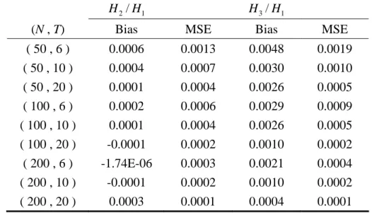
look at the performance of the allocative parameters, estimated in the first step. One

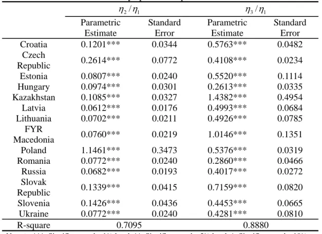
thing that is immediately noticeable is that H₂/H and ₁ H₃/H are well estimated ₁

even for the case of the smallest sample size, i.e., (N, T) = (50, 6). Another desirable

feature is that the bias and the MSE fall when either N or T increases, aside from the

bias of H₂/H when N = 200. Even in those exceptional cases the biases are ₁

negligible.

Table 1. The performance of the allocative parameter estimates setting M(‧)=2 ln(1y1)

2/ 1

H H H₃/H ₁

(N , T) Bias MSE Bias MSE ( 50 , 6 ) 0.0006 0.0013 0.0048 0.0019 ( 50 , 10 ) 0.0004 0.0007 0.0030 0.0010 ( 50 , 20 ) 0.0001 0.0004 0.0026 0.0005 ( 100 , 6 ) 0.0002 0.0006 0.0029 0.0009 ( 100 , 10 ) 0.0001 0.0004 0.0026 0.0005 ( 100 , 20 ) -0.0001 0.0002 0.0010 0.0002 ( 200 , 6 ) -1.74E-06 0.0003 0.0021 0.0004 ( 200 , 10 ) -0.0001 0.0002 0.0010 0.0002 ( 200 , 20 ) 0.0003 0.0001 0.0004 0.0001

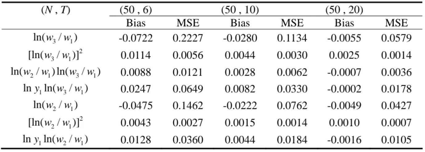
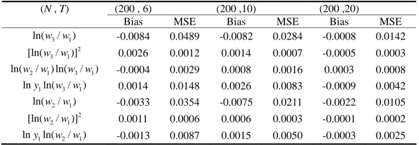
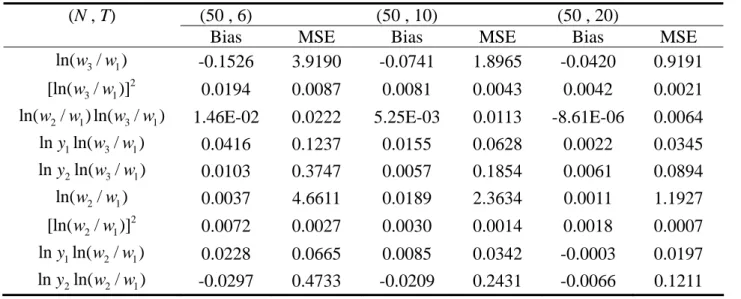
Table 2 reveals that in general the MSEs of the parameter estimates of the

parametric portion fall quickly when either N or T increases. For instance, when

fixing N = 50, the MSE of the coefficient of ln(w₃/w shrinks swiftly from 0.2227 ₁)

to 0.0579 as T increases from 6 to 20. The figure continues to fall to 0.0142 when (N,

T) = (200, 20). In addition, the bias measures exhibit a similar pattern, although the

biases of some coefficients are a little large in the case of (N, T) = (50, 6) relative to

their true values. In summary, the estimators in the first step perform quite well as

expected in terms of their biases and MSEs, which improve when either N or T

increases.

Table 2. The performance of the parameter estimates in Step 1 setting M(‧)=2 ln(1y₁)

(N , T) (50 , 6) (50 , 10) (50 , 20)

Bias MSE Bias MSE Bias MSE

3 1 ln(w /w ) -0.0722 0.2227 -0.0280 0.1134 -0.0055 0.0579 2 3 1 [ln(w /w)] 0.0114 0.0056 0.0044 0.0030 0.0025 0.0014 2 1 3 1 ln(w /w) ln(w /w) 0.0088 0.0121 0.0028 0.0062 -0.0007 0.0036 1 3 1 lny ln(w /w ) 0.0247 0.0649 0.0082 0.0330 -0.0002 0.0178 2 1 ln(w /w ) -0.0475 0.1462 -0.0222 0.0762 -0.0049 0.0427 2 2 1 [ln(w /w)] 0.0043 0.0027 0.0015 0.0014 0.0010 0.0007 1 2 1 lny ln(w /w ) 0.0128 0.0360 0.0044 0.0184 -0.0016 0.0105 (N , T) (100 , 6) (100, 10) (100, 20)

Bias MSE Bias MSE Bias MSE

3 1 ln(w /w ) -0.0179 0.0935 -0.0055 0.0579 -0.0082 0.0284 2 3 1 [ln(w /w)] 0.0036 0.0025 0.0025 0.0014 0.0014 0.0007 2 1 3 1 ln(w /w) ln(w /w) 0.0015 0.0052 -0.0007 0.0036 0.0008 0.0016 1 3 1 lny ln(w /w ) 0.0046 0.0276 -0.0002 0.0178 0.0026 0.0083 2 1 ln(w /w ) -0.0171 0.0679 -0.0049 0.0427 -0.0075 0.0211 2 2 1 [ln(w /w)] 0.0011 0.0012 0.0010 0.0007 0.0006 0.0003 1 2 1 lny ln(w /w ) 0.0023 0.0157 -0.0016 0.0105 0.0015 0.0050

(N , T) (200 , 6) (200 ,10) (200 ,20)

Bias MSE Bias MSE Bias MSE

3 1 ln(w /w ) -0.0084 0.0489 -0.0082 0.0284 -0.0008 0.0142 2 3 1 [ln(w /w)] 0.0026 0.0012 0.0014 0.0007 -0.0005 0.0003 2 1 3 1 ln(w /w) ln(w /w) -0.0004 0.0029 0.0008 0.0016 0.0003 0.0008 1 3 1 lny ln(w /w ) 0.0014 0.0148 0.0026 0.0083 -0.0009 0.0042 2 1 ln(w /w ) -0.0033 0.0354 -0.0075 0.0211 -0.0022 0.0105 2 2 1 [ln(w /w)] 0.0011 0.0006 0.0006 0.0003 -0.0001 0.0002 1 2 1 lny ln(w /w ) -0.0013 0.0087 0.0015 0.0050 -0.0003 0.0025

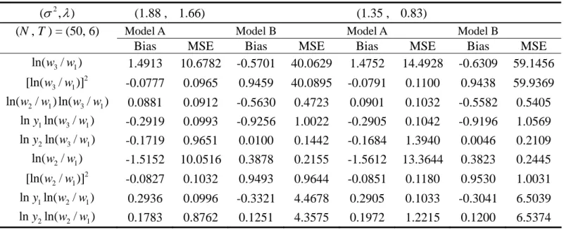
Table 3 presents the biases and MSEs of the parametric part for Models A and B

obtained from Step 3. Generally speaking, these estimators perform poorly. Their

biases and MSEs are much larger than those derived from the first-stage estimation. In

addition, the biases and MSEs of Model A decrease to some extent as the sample size

increases, while the biases of Model B are hardly altered with an the increase in the

sample size. This leads us to conclude that the computationally simple first-stage

estimators of the parametric part outperform the third-step estimators of Models A and

B. Does this imply that Step 3 is redundant? The answer is no. It is necessary for the

estimation of the distribution parameters. Please see below.

The distribution parameters of v and U are estimated in Step 5 by the maximum

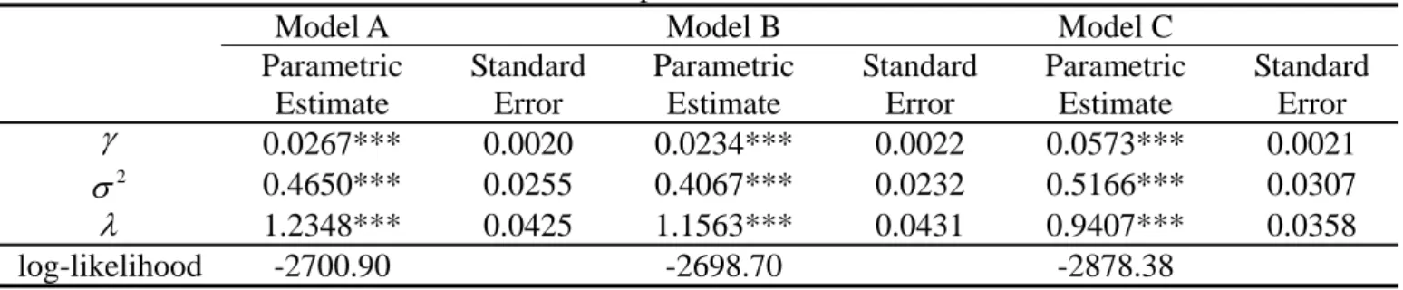
likelihood, and Table 4 presents the results. The estimators of Model C have larger

biases and MSEs in comparison with those of Models A and B in most cases. We

therefore drop Model C from now on whenever not necessary and focus our analysis

only on Models A and B. For the case of (2,) = (1.88, 1.66), despite the fact that Model B’s estimator of  has lower biases and MSEs than Model A does in almost all cases, though the differences are quite small. Model B’s estimator of 2 performs slightly better than Model A’s, while the reverse is true for the estimator of

. It is a caveat that Model A’s estimator of 2 tends to have a larger variation when the sample size is small. As far as the estimator of smooth function M(‧) is

concerned, Model A is found to be superior to Model B since Model A yields much

smaller biases and MSEs than Model B does in most cases. Only for the cases of a

large time period (T = 20) are Model B’s biases a little less than Model A. Turning to

the cases of (2,) = (1.35, 0.83) and (1.63, 1.24), the results are rather similar to the preceding case.

Table 3. The performance of the parameter estimates from the third-stage setting M(‧)=2 ln(1y1) 2

( , ) _{(1.88 , 1.66) (1.35 , 0.83) (1.63 , 1.24)}

( N , T ) = (50, 6) Model A Model B Model A Model B Model A Model B

Bias MSE Bias MSE Bias MSE Bias MSE Bias MSE Bias MSE

3 1 ln(w /w ) 1.0484 1.2796 -0.4020 0.8330 1.0470 1.3472 -0.3920 1.1417 1.0479 1.2987 -0.3980 0.9200 2 3 1 [ln(w /w)] -0.0298 0.0821 0.7398 1.1935 -0.0305 0.0986 0.7337 1.4732 -0.0297 0.0870 0.7373 1.2713 2 1 3 1 ln(w /w) ln(w /w) 0.0373 0.0796 -0.5661 0.4531 0.0390 0.0946 -0.5619 0.5130 0.0376 0.0841 -0.5644 0.4700 1 3 1 lny ln(w /w ) -0.3118 0.1117 -0.9281 0.9856 -0.3116 0.1173 -0.9220 1.0320 -0.3118 0.1133 -0.9256 0.9973 2 1 ln(w /w ) -1.0744 1.3335 0.2129 0.1685 -1.0684 1.3968 0.2077 0.2251 -1.0721 1.3505 0.2108 0.1845 2 2 1 [ln(w /w)] -0.0349 0.0912 0.7478 0.6114 -0.0375 0.1090 0.7458 0.6336 -0.0356 0.0965 0.7470 0.6174 1 2 1 lny ln(w /w ) 0.3191 0.1162 0.1947 0.0879 0.3173 0.1211 0.1952 0.1108 0.3184 0.1175 0.1949 0.0944 2 ( , ) (1.88 , 1.66) (1.35 , 0.83) _{(1.63 , 1.24)}

( N , T ) = (50, 10) Model A Model B Model A Model B Model A Model B

Bias MSE Bias MSE Bias MSE Bias MSE Bias MSE Bias MSE

3 1 ln(w /w ) 0.8685 0.8114 -0.3865 0.3834 0.8724 0.8423 -0.3911 0.4996 0.8701 0.8204 -0.3884 0.4148 2 3 1 [ln(w /w)] -0.0098 0.0368 0.7075 0.7116 -0.0106 0.0441 0.7142 0.8225 -0.0099 0.0389 0.7102 0.7419 2 1 3 1 ln(w /w) ln(w /w) 0.0106 0.0367 -0.5500 0.3446 0.0113 0.0430 -0.5482 0.3638 0.0108 0.0385 -0.5493 0.3494 1 3 1 lny ln(w /w ) -0.2588 0.0716 -0.9175 0.8822 -0.2599 0.0740 -0.9161 0.8999 -0.2592 0.0723 -0.9170 0.8865 2 1 ln(w /w ) -0.9118 0.8920 0.1990 0.0788 -0.9134 0.9214 0.1974 0.0979 -0.9125 0.9003 0.1984 0.0837 2 2 1 [ln(w /w)] -0.0115 0.0405 0.7459 0.5752 -0.0120 0.0475 0.7476 0.5863 -0.0115 0.0425 0.7466 0.5785 1 2 1 lny ln(w /w ) 0.2715 0.0786 0.2028 0.0580 0.2719 0.0810 0.2006 0.0647 0.2717 0.0793 0.2020 0.0596

2

( , ) (1.88 , 1.66) (1.35 , 0.83) _{(1.63 , 1.24)}

( N , T ) = (50, 20) Model A Model B Model A Model B Model A Model B

Bias MSE Bias MSE Bias MSE Bias MSE Bias MSE Bias MSE

3 1 ln(w /w ) 0.6812 0.4800 -0.4096 0.2192 0.6831 0.4885 -0.4090 0.2419 0.6819 0.4824 -0.4093 0.2245 2 3 1 [ln(w /w)] -0.0011 0.0167 0.7320 0.5860 -0.0012 0.0180 0.7331 0.6097 -0.0011 0.0170 0.7323 0.5917 2 1 3 1 ln(w /w) ln(w /w) 0.0016 0.0169 -0.5532 0.3160 0.0015 0.0182 -0.5507 0.3175 0.0015 0.0172 -0.5522 0.3159 1 3 1 lny ln(w /w ) -0.2027 0.0423 -0.9217 0.8594 -0.2032 0.0430 -0.9194 0.8592 -0.2028 0.0425 -0.9208 0.8587 2 1 ln(w /w ) -0.7134 0.5246 0.2025 0.0505 -0.7137 0.5309 0.2001 0.0535 -0.7135 0.5262 0.2016 0.0511 2 2 1 [ln(w /w)] -0.0021 0.0180 0.7522 0.5699 -0.0020 0.0196 0.7524 0.5720 -0.0020 0.0184 0.7523 0.5704 1 2 1 lny ln(w /w ) 0.2122 0.0462 0.1966 0.0425 0.2122 0.0467 0.1960 0.0440 0.2122 0.0463 0.1964 0.0429 2 ( , ) (1.88 , 1.66) (1.35 , 0.83) _{(1.63 , 1.24)}

( N , T ) = (100, 6) Model A Model B Model A Model B Model A Model B

Bias MSE Bias MSE Bias MSE Bias MSE Bias MSE Bias MSE

3 1 ln(w /w ) 0.8227 0.7571 -0.3908 0.4784 0.8286 0.8027 -0.3999 0.6393 0.8250 0.7712 -0.3944 0.5251 2 3 1 [ln(w /w)] -0.0078 0.0404 0.7216 0.8238 -0.0089 0.0500 0.7323 0.9832 -0.0081 0.0433 0.7258 0.8709 2 1 3 1 ln(w /w) ln(w /w) 0.0083 0.0400 -0.5468 0.3606 0.0094 0.0482 -0.5441 0.3881 0.0085 0.0425 -0.5458 0.3682 1 3 1 lny ln(w /w ) -0.2446 0.0661 -0.9165 0.8992 -0.2462 0.0697 -0.9139 0.9232 -0.2452 0.0672 -0.9155 0.9056 2 1 ln(w /w ) -0.8548 0.8141 0.1972 0.0970 -0.8587 0.8568 0.1945 0.1242 -0.8563 0.8271 0.1961 0.1048 2 2 1 [ln(w /w)] -0.0079 0.0440 0.7469 0.5831 -0.0091 0.0531 0.7501 0.5998 -0.0082 0.0467 0.7482 0.5883 1 2 1 lny ln(w /w ) 0.2536 0.0709 0.1990 0.0630 0.2548 0.0743 0.1953 0.0724 0.2541 0.0719 0.1975 0.0655

2

( , ) (1.88 , 1.66) (1.35 , 0.83) _{(1.63 , 1.24)}

( N , T ) = (100, 10) Model A Model B Model A Model B Model A Model B

Bias MSE Bias MSE Bias MSE Bias MSE Bias MSE Bias MSE

3 1 ln(w /w ) 0.6792 0.4909 -0.3976 0.2700 0.6828 0.5104 -0.3997 0.3295 0.6806 0.4967 -0.3984 0.2861 2 3 1 [ln(w /w)] -0.0019 0.0186 0.7234 0.6283 -0.0022 0.0221 0.7275 0.6892 -0.0019 0.0196 0.7250 0.6452 2 1 3 1 ln(w /w) ln(w /w) 0.0028 0.0188 -0.5493 0.3237 0.0029 0.0220 -0.5464 0.3312 0.0028 0.0197 -0.5482 0.3253 1 3 1 lny ln(w /w ) -0.2019 0.0431 -0.9174 0.8632 -0.2029 0.0447 -0.9147 0.8688 -0.2023 0.0436 -0.9164 0.8642 2 1 ln(w /w ) -0.7082 0.5319 0.1985 0.0602 -0.7098 0.5489 0.1956 0.0692 -0.7089 0.5368 0.1974 0.0625 2 2 1 [ln(w /w)] -0.0035 0.0208 0.7490 0.5698 -0.0036 0.0245 0.7501 0.5763 -0.0034 0.0218 0.7494 0.5718 1 2 1 lny ln(w /w ) 0.2103 0.0466 0.1987 0.0477 0.2108 0.0480 0.1970 0.0515 0.2105 0.0470 0.1980 0.0486 2 ( , ) (1.88 , 1.66) (1.35 , 0.83) _{(1.63 , 1.24)}

( N , T ) = (100, 20) Model A Model B Model A Model B Model A Model B

Bias MSE Bias MSE Bias MSE Bias MSE Bias MSE Bias MSE

3 1 ln(w /w ) 0.5231 0.2817 -0.3974 0.1864 0.5242 0.2861 -0.3972 0.1949 0.5235 0.2829 -0.3974 0.1864 2 3 1 [ln(w /w)] 0.0009 0.0076 0.7203 0.5472 0.0013 0.0081 0.7209 0.5566 0.0011 0.0077 0.7203 0.5472 2 1 3 1 ln(w /w) ln(w /w) -0.0017 0.0076 -0.5471 0.3047 -0.0020 0.0081 -0.5461 0.3052 -0.0018 0.0077 -0.5471 0.3047 1 3 1 lny ln(w /w ) -0.1552 0.0247 -0.9181 0.8483 -0.1556 0.0251 -0.9170 0.8477 -0.1554 0.0248 -0.9181 0.8483 2 1 ln(w /w ) -0.5457 0.3055 0.1975 0.0441 -0.5458 0.3085 0.1964 0.0452 -0.5458 0.3063 0.1975 0.0441 2 2 1 [ln(w /w)] 0.0021 0.0081 0.7496 0.5642 0.0023 0.0087 0.7498 0.5651 0.0022 0.0083 0.7496 0.5642 1 2 1 lny ln(w /w ) 0.1622 0.0269 0.1997 0.0421 0.1623 0.0272 0.1993 0.0426 0.1623 0.0270 0.1997 0.0421

2

( , ) (1.88 , 1.66) (1.35 , 0.83) _{(1.63 , 1.24)}

( N , T ) = (200, 6) Model A Model B Model A Model B Model A Model B

Bias MSE Bias MSE Bias MSE Bias MSE Bias MSE Bias MSE

3 1 ln(w /w ) 0.6314 0.4391 -0.3838 0.3063 0.6342 0.4613 -0.3847 0.3769 0.6325 0.4458 -0.3842 0.3260 2 3 1 [ln(w /w)] -0.0003 0.0184 0.7112 0.6546 0.0004 0.0226 0.7145 0.7277 0.0001 0.0196 0.7125 0.6755 2 1 3 1 ln(w /w) ln(w /w) 0.0003 0.0181 -0.5413 0.3237 -5.45E-06 0.0219 -0.5389 0.3356 0.0001 0.0192 -0.5404 0.3269 1 3 1 lny ln(w /w ) -0.1877 0.0384 -0.9113 0.8611 -0.1886 0.0402 -0.9080 0.8685 -0.1880 0.0390 -0.9100 0.8626 2 1 ln(w /w ) -0.6563 0.4722 0.1914 0.0661 -0.6566 0.4904 0.1884 0.0782 -0.6565 0.4774 0.1903 0.0695 2 2 1 [ln(w /w)] -0.0002 0.0201 0.7459 0.5689 -0.0005 0.0244 0.7469 0.5762 -0.0002 0.0213 0.7463 0.5712 1 2 1 lny ln(w /w ) 0.1948 0.0412 0.2014 0.0523 0.1951 0.0428 0.1998 0.0571 0.1949 0.0417 0.2008 0.0536 2 ( , ) (1.88 , 1.66) (1.35 , 0.83) _{(1.63 , 1.24)}

( N , T ) = (200, 10) Model A Model B Model A Model B Model A Model B

Bias MSE Bias MSE Bias MSE Bias MSE Bias MSE Bias MSE

3 1 ln(w /w ) 0.5261 0.2911 -0.3955 0.2086 0.5274 0.3000 -0.3955 0.2355 0.5265 0.2936 -0.3955 0.2157 2 3 1 [ln(w /w)] 0.0008 0.0083 0.7221 0.5714 0.0013 0.0099 0.7230 0.6002 0.0010 0.0088 0.7224 0.5792 2 1 3 1 ln(w /w) ln(w /w) 0.0003 0.0084 -0.5484 0.3112 -0.0005 0.0097 -0.5456 0.3135 0.0000 0.0087 -0.5473 0.3114 1 3 1 lny ln(w /w ) -0.1563 0.0256 -0.9162 0.8497 -0.1566 0.0263 -0.9137 0.8503 -0.1564 0.0258 -0.9153 0.8494 2 1 ln(w /w ) -0.5441 0.3102 0.1974 0.0488 -0.5444 0.3174 0.1946 0.0528 -0.5442 0.3122 0.1963 0.0498 2 2 1 [ln(w /w)] -0.0013 0.0094 0.7488 0.5648 -0.0006 0.0109 0.7493 0.5678 -0.0010 0.0098 0.7490 0.5657 1 2 1 lny ln(w /w ) 0.1615 0.0272 0.1989 0.0435 0.1617 0.0278 0.1982 0.0454 0.1616 0.0274 0.1986 0.0440

2

( , ) (1.88 , 1.66) (1.35 , 0.83) _{(1.63 , 1.24)}

( N , T ) = (200, 20) Model A Model B Model A Model B Model A Model B

Bias MSE Bias MSE Bias MSE Bias MSE Bias MSE Bias MSE

3 1 ln(w /w ) 0.4047 0.1674 -0.4005 0.1729 0.4054 0.1695 -0.4010 0.1792 0.4049 0.1680 -0.4007 0.1745 2 3 1 [ln(w /w)] -0.0007 0.0036 0.7215 0.5323 -0.0011 0.0039 0.7224 0.5395 -0.0008 0.0037 0.7218 0.5343 2 1 3 1 ln(w /w) ln(w /w) -4.81E-05 0.0037 -0.5495 0.3044 0.0004 0.0039 -0.5497 0.3056 0.0001 0.0037 -0.5496 0.3047 1 3 1 lny ln(w /w ) -0.1199 0.0147 -0.9208 0.8503 -0.1201 0.0148 -0.9209 0.8515 -0.1200 0.0147 -0.9209 0.8506 2 1 ln(w /w ) -0.4240 0.1835 0.2002 0.0424 -0.4243 0.1852 0.2003 0.0434 -0.4241 0.1840 0.2002 0.0426 2 2 1 [ln(w /w)] 0.0007 0.0039 0.7501 0.5636 0.0002 0.0042 0.7502 0.5642 0.0005 0.0040 0.7501 0.5638 1 2 1 lny ln(w /w ) 0.1258 0.0161 0.1997 0.0408 0.1258 0.0162 0.1995 0.0412 0.4049 0.1680 -0.4007 0.1745

Although both Models A and B perform reasonably well, the simulation results

appear to be in favor of an advantage for Model A in general and for the estimation of

TE scores in particular (see Tables 7 and 14 below). Comparing (3-13) with (4-1), one

can tell that their disparity originates from how  and lnG are estimated. For _nt Model A, they are estimated by NISUR viewing parameters contained in lnG as _nt

unknown, while for Model B lnG is replaced by _nt lnGˆ_nt leaving  to be

estimated by OLS. The superiority of Model A may be explained by its allowance for

the presence of lnG in the expenditure equation. _nt

It is apparent from Table 4 that Model C gives rise to undesirable estimators of

( ,2, ). This is mainly ascribable to the fact that it overlooks Step 3 and proceeds from Step 2 directly to Steps 4 and 5. By doing so, the residual of (4-2) is indirectly

derived using the NISUR estimates of lnGˆ_nt and ˆ , which are obtained by

simultaneously estimating the (J 1) share equations, instead of the expenditure equation. Conversely, the residuals of (3-13) and (4-1) corresponding to Models A and

B, respectively, are directly deduced from estimating the expenditure equation. Step 3

is thus necessary.

We have learned from Tables 2 and 3 that the parameter estimates of the

parametric part of the cost function obtained in the first step outperform those

obtained in the third step. These estimates are applied to compute lnG . We now _nt

compare the performance of the estimated lnG to gain further insight into the _nt

properties of alternative models. Not surprisingly, G1 has smaller biases and MSEs

than G2A and G2B, derived from Models A and B, respectively, in almost all (N, T)

and (2,) combinations. The outcomes support the use of G1 as the estimate of lnG . _nt